Model Simulations of a Shock-Cloud Interaction in the Cygnus Loop

Abstract

We present optical observations and 2D hydrodynamic modeling of an isolated shocked ISM cloud. H$\alpha$ images taken in 1992.6 and 2003.7 of a small optical emission cloud along the southwestern limb of the Cygnus Loop were used to measure positional displacements of $\sim$ $0\farcs 1$ yr^-1 for surrounding Balmer dominated emission filaments and $0\farcs 025-\farcs 055$ yr^-1 for internal cloud emission features. These measurements imply transverse velocities of $\simeq$ 250 km s^-1 and $\simeq$ 80 – 140 km s^-1 for ambient ISM and internal cloud shocks respectively. A lack of observed turbulent gas stripping at the cloud–ISM boundary in the H$\alpha$ images suggests that there is not an abrupt density change at the cloud–ISM boundary. Also, the complex shock structure visible within the cloud indicates that the cloud’s internal density distribution is two phased: a smoothly varying background density which is populated by higher density clumps.

Guided by the H$\alpha$ images, we present model results for a shock interacting with a non-uniform ISM cloud. We find that this cloud can be well modeled by a smoothly varying power law core with a density contrast of $\sim$ 4 times the ambient density, surrounded by a low density envelope with a Lorentzian profile. The lack of sharp density gradients in such a model inhibits the growth of Kelvin-Helmholtz instabilities, consistent with the cloud’s appearance. Our model results also suggest that cloud clumps have densities $\sim$ 10 times the ambient ISM density and account for $\sim$ 30% of the total cloud volume. Moreover, the observed spacing of internal cloud shocks and model simulations indicate that the distance between clumps is $\sim$ 4 clump radii. We conclude that this diffuse ISM cloud is best modeled by a smoothly varying, low density distribution coupled to higher density, moderately spaced internal clumps.

1. Introduction

The interaction of shock waves with the interstellar medium (ISM) such as those associated with supernovae, stellar winds, bipolar flows, H II regions, or spiral density waves is a fundamental process in interstellar gas dynamics and is key to understanding the evolution and structure of the ISM. The highly nonlinear interaction between supernova generated shocks and interstellar clouds is often not suited to analytic approaches but requires a multidimensional hydrodynamics study of the shock-cloud problem using high resolution methods.

A hydrodynamical study of a shocked ISM cloud was made by Klein, McKee, & Colella (1994, hereafter KMC94), who found that the cloud may be destroyed by a series of instabilities associated with the post-shock flow of inter-cloud gas past the cloud. Earlier work on this problem includes that of Woodward (1976) and Nittman, Falle, & Gaskell (1982). More recently, Poludnenko, Frank, & Blackman (2002) studied the role that internal cloud structure plays in the destruction of the cloud.

For investigating shocked ISM cloud physics, the interaction between a supernova (SN) shock and low density diffuse ISM clouds is of particular interest. Supernova remnants (SNRs) shape and enrich the chemical and dynamical structure of the ISM which, in turn, affect the evolution of subsequent SNRs. The details of just how SN generated shock waves interact with interstellar clouds are not well understood.

There are several limiting factors in attempting to compare model simulations to observed SNR shock cloud interactions. While models can be viewed edge on and rotated in two or three dimensions, shocked interstellar clouds are viewed only in projection, which leads to a complex appearing shock structure due to multiple and overlapping shocks. In addition, one observes only a single epoch, i.e., a ‘snapshot’, of the interaction. These factors make it difficult to understand and model the time dependent kinematics and detailed dynamical processes of the interaction. Also, unlike how they are often modeled, real interstellar clouds are neither cylindrical or spherical in shape nor sharp edged, with interiors very likely non-uniform in density. Furthermore, many shocked interstellar clouds are dense enough so that radiative losses, which can alter the overall dynamics of the shock-cloud interaction, are important (Mellema et al., 2002; Fragile et al., 2004). Finally, the inclusion of an embedded magnetic field can drastically alter the dynamics of the interaction. For instance, a strong, ordered magnetic field can suppress dynamical instability growth predicted by fluid dynamical simulations (Mac Low et al., 1994; Fragile et al., 2005).

In looking for an ‘ideal’ shock-cloud interaction, one would like to avoid many of the aforementioned effects and the Cygnus Loop supernova remnant affords several distinct advantages. Because of the remnant’s large angular size (2.8${}^{\circ}\times$ 3.5^∘), low foreground extinction ($E[B-V]=0.08$ mag; Parker 1967; Fesen, Blair, & Kirshner 1982), and wide range of shock conditions, the Cygnus Loop is one of the better locations for studying the ISM shock physics of middle-aged remnants. At a distance of 550${}_{-80}^{+110}$ pc (Blair et al., 2005), it has a physical size of 27 $\times$ 33.5 pc. Located 8.5^∘ below the galactic plane, the remnant lies in a multi-phase medium containing large ISM clouds with a hydrogen density of $n=5-10$ cm^-3, surrounded by a lower density inter-cloud component of $n\approx 0.1-0.2$ cm^-3 (DeNoyer, 1975).

Recently, Patnaude et al. (2002) studied a small, isolated cloud along the southwest limb of the Cygnus Loop which met many of the desired cloud properties for investigating shock-cloud interactions. This cloud is relatively small ($\sim$ 2$\arcmin$ in radius; $0.32$ pc at $550$ pc; Blair et al., 2005), exhibits a fairly uncomplicated, line-of-sight internal structure, and lies isolated from other shocked ISM clouds. Moreover, the shock-cloud interaction is dominated by non-radiative, or ‘Balmer-dominated’ filaments, indicating that the cloud-shock dynamics is not significantly affected by post-shock radiative losses.

Here we present a new analysis of this small shocked cloud. Proper motion measurements and inferred shock velocities of individual filaments in and surrounding the cloud are presented. These results were used to estimate the initial conditions for hydrodynamical model simulations of a shock interaction with an unmagnetized, lumpy cloud. In $\S 2$, these new observations are presented as well as the technique used to measure the filament proper motions. Model parameter estimates are then discussed in $\S 3$. Our hydrodynamical models are presented in $\S 4$, where proper motion and density estimates are implemented in the model initial conditions. Model results are presented in $\S 5$, and they are compared to the southwest cloud in $\S 6$ with our conclusions in $\S 7$.

2. Observations

Narrow passband H$\alpha$ images of the southwest region of the Cygnus Loop were obtained on 7 July 1992 and 29 August 2003 using the MDM 2.4 m Hiltner telescope. For the July 1992 images, four 600 s H$\alpha$ filter (FWHM = 80 Å) exposures were acquired with a Loral 2048 $\times$ 2048 front side illuminated CCD yielding a spatial resolution of $0\farcs 343$ pixel^-1. Details of the 1992 observations and subsequent data reduction can be found in Patnaude et al. (2002).

Two 1000 s H$\alpha$ filter (FWHM = 15 Å) exposures were taken in August 2003 with a SITe 2048 $\times$ 2048 back side illuminated CCD with a resolution of $0\farcs 275$ pixel^-1. Using IRAF, the data were bias-subtracted, flat-fielded, and cosmic-ray hits were removed. The resulting 2003 epoch image is shown in Figure 1. Globally, the cloud’s morphology is nearly identical to that seen in the 1992 images (Figs. 2 & 3 Patnaude et al., 2002), but close inspection between the two epoch images showed measurable proper motions for both internal cloud structures and the surrounding thin shock front filaments.

3. Analysis and Results

Following the procedure described by Thorstensen, Fesen, & van den Bergh (2001), the coordinate systems of the two H$\alpha$ images were aligned using DAOPHOT in conjunction with the USNO-A2.0 catalog. The datasets were then rebinned to an effective image scale of $0\farcs 1$ pix^-1. This rebinning introduced a small global offset of $-0\farcs 07$ pix^-1 between the two images, uniform across the entire field of view.

3.1. Proper Motion Measurements

Individual filament regions for the proper motion analysis were selected based on their projection onto the plane of the sky, the complexity of the filament and surrounding regions, and the brightness of the filament feature. Based on these criteria, 14 filaments within the cloud, including both Balmer dominated and radiative filaments, and 21 regions from the surrounding Balmer dominated shock front were chosen (see Figure 1).

One-dimensional intensity profiles were extracted for each region and the pixel shift in each shock filament was computed using the IRAF task xcsao, which is based on the software of Tonry & Davis (1979). While this task was written to compute relative radial velocities via the cross-correlation function between two spectra, the cross-correlation function yields accurate filament motions in terms pixel shifts between two images. For thin Balmer-dominated filaments and bright and sharp cloud shock features, the cross-correlation analysis was able to match the shock fronts between the two epochs and measure the pixel shift between the two data sets to an accuracy of 10% – 15%. The results from this analysis are listed in terms of proper motion (mas yr^-1) and transverse velocity (km s^-1) in Table 1. The quoted velocities assume a distance of 550${}_{-80}^{+110}$ pc (Blair et al., 2005).

Example data and cross-correlation functions for two regions are shown in Figure 2. These one-dimensional filaments and cross-correlation functions are representative of the data for the non-radiative filaments (Fig. 2, left) and internal cloud filaments (Fig. 2, right), where there is often a plateau of emission (from shocked cloud material) downstream from the shock front and then a steep rise in emission at the cloud shock front.

Quoted errors in Table 1 include the signal to noise in the filament region, the curvature of the filament region, the profile of the filament when convolved with the image PSF (FWHM₁₉₉₂ = $1\farcs 0$; FWHM₂₀₀₃ = $0\farcs 7$), and the contribution from the background, local nebulosity, and adjacent filaments. For well resolved filaments, the cumulative effect of these errors is $\sim$ 0.6 pixel, or about 10 km s^-1.

3.2. Estimate of Cloud Parameters

As discussed in Patnaude et al. (2002), this shock-cloud interaction is nearly tangent along the line of sight to the southwestern limb of the southern region of the Cygnus Loop. The cloud is being run over by the remnant’s shock front which is moving roughly east-west. We have divided the cloud into two regions: the ISM shock front and the cloud-shock region. Based on the filament velocities listed in Table 1, we estimated an interstellar shock velocity of 250 km s^-1 associated with the Balmer-dominated filaments. The wide range of Balmer filament velocities observed ($140-260$ km s^-1) may be due in part to density fluctuations around the cloud and the fact that only one component of the filament velocity is measured. That is, for filaments which are highly curved, the space velocity of the shock might be 200 km s^-1, but the local measured velocity might be in a direction other than perpendicular to our line of sight. Furthermore, though filaments were chosen based upon selective criteria, factors such as low signal to noise as well as adjacent, overlapping filaments contributed in some cases to a poorer cross-correlation between the two images. Nonetheless, our estimated shock velocity $\simeq$250 km s^-1 is consistent with the X-ray shock velocity of $\sim$ 300 km s^-1 inferred from the ROSAT PSPC measurements (Patnaude et al., 2002).

The shocked cloud can be further divided into regions where the cloud-shock is interacting with the cloud, and where it is interacting with cloud clumps or “cloudlets”. In general, the inferred shock velocities vary widely (65–140 km s^-1). This suggests that the density structure of the cloud is fairly complex, as the cloud-shock appears to have been slowed less in certain areas relative to others.

Based on these measurements, we adopt a shock velocity range inside the cloud of $60-100$ km s^-1. These estimated cloud-shock velocities in turn imply a range of density contrasts in the cloud. Assuming ram pressure equilibrium, ($\rho_{a}v^{2}_{s}\approx\rho_{c}v^{2}_{cs}$) the density contrast between the cloud and the ambient medium, $\chi$ $\equiv$ $\rho_{c}/\rho_{a}$, is $\sim$ 4–17, with higher values representing areas populated with cloudlets, and lower values representing regions of low density within the cloud.

The low density nature of this cloud permits us to view its internal shock dynamics. We have used the structure and spacing of the internal shock fronts to estimate the clumpiness of the cloud. The easiest place to do this is at the western nose of the cloud (Regions C8–C10). Measurements suggest that the post-shock spacing of clumps in the cloud is $\sim$ 10$\arcsec$ – 30$\arcsec$. The upper limits corresponds to shocks which are more highly evolved, while the lower limit corresponds to ‘small’ shocks. Based on the size of the cloud (2$\arcmin$ – 4$\arcmin$ diameter), the cloudlets likely account for 30% of the total cloud volume. Furthermore, based on a maximum compression of $\sim$ 4 for cloud clumps, we estimate the spacing between cloudlets to be $\approx$ 4–5 cloudlet radii ($a_{cloudlet}$).

4. Hydrodynamical Models

For modeling this shock-cloud interaction, we have used the numerical hydrodynamics software VH-1 (Blondin & Knerr, 1992; Stevens et al., 1992), which implements the piecewise parabolic method (PPM) to solve the equations of gas dynamics (Colella, & Woodward, 1984). The PPM approach incorporates a fixed computational grid to evolve the standard conservation equations of mass, momentum, and energy. We assume an ideal, inviscid fluid with a ratio of specific heats, $\gamma$, equal to $5/3$. VH-1 does not explicitly treat the collisionless shock physics associated with Balmer-dominated shocks. However, the goal of this study is to understand how a blast wave interacts with a diffuse ISM cloud. For these purposes, VH-1 serves as an excellent tool for tracing the motion and dynamics of this interaction.

Simulations were performed on a 1440 $\times$ 1440 Cartesian grid. The fiducial physical size of the square grid is 1 $\times$ 1, with dx = dy = 6.9 $\times$ 10^-4, The size of the cloud sets the scale of the models. The cloud is $\approx$ 2$\arcmin$ in radius ($\approx$ 10¹⁸ cm $\times$ d${}_{550\,\,{\mathrm{p}c}}$). On average, the cloud radius is 30% of the computational grid, or $\approx$ 450 cells per cloud radius. Therefore, the physical length scale of the grid $\Delta$x $\approx$ 2 $\times$ 10¹⁵ cm cell^-1.

We estimate the importance of radiative losses by calculating the cooling time scale and comparing it to dynamically relevant time scales (mainly, the cloud crushing time and the pressure variation time scale). In general, radiative losses will be considered important if the cooling time is comparable to or shorter than the cloud crushing time. We estimate the cooling time using the approximation of Kahn (1976), $t_{cool}$ = $Cv^{3}/\rho$, where $v$ is the cloud shock velocity in units of km s^-1, $\rho$ is the cloud density in units of gm cm^-3, and $C$ is a constant $=$ 6.0 $\times$ 10^-35. Assuming a cloud shock velocity of 140 km s^-1 and a cloud density of 10^-24 gm cm^-3, we estimate a cooling time $t_{cool}$ $>$ 5000 yr. In contrast, the cloud crushing time, $t_{cc}$ $\equiv$ $\chi^{1/2}a_{0}/v_{b}$, is $\approx$ 3800 yr, for a blast wave velocity of 250 km s^-1 and an initial cloud radius of $a_{0}$ = 0.3 pc. Furthermore, the pressure variation time scale is $\sim$ 0.1$t_{cc}$ (KMC94), which is $<$ $t_{cool}$. Thus, it appears that neglecting the effects of cooling in our models will not have a significant impact on our results. This is supported by Patnaude et al. (2002) who showed that this cloud is only weakly radiative.

Under the assumptions that radiative losses are not dynamically important and that magnetic fields are not present (or that the cloud is only weakly magnetized), the shock-cloud interaction can be wholly defined by two parameters (KMC94), the shock Mach number, and $\chi$, the density contrast of the cloud. Assuming an ISM sound speed of $\approx$ 10–15 km s^-1 and a blast wave velocity of 250 km s^-1, we estimate a shock Mach number of $M$ $\approx$ 20. Furthermore, as pointed out in $\S 3$, we estimate a cloud to ISM density contrast of $\chi$ $\approx$ 6.

To further simplify the problem, we chose a set of non-dimensional variables such that the ISM density $\rho_{a}$ is set to the ratio of specific heats, $\gamma$ = $5/3$, and the ISM pressure, $P_{a}$, is set to unity. The ISM sound speed, $c_{a}$, is thus set to 1 ($c_{a}$ = $(\gamma P_{a}/\rho_{a})^{1/2}$), and the shock velocity $v_{b}$ is just the shock Mach number.

Model results by KMC94 suggested that a cloud radius should be at least of order 120 cells. For our models here, we chose the main cloud to have a radius of 300-500 cells ($\simeq$ 10^17-18 cm). The internal cloudlets have sizes which are 10–20% of the cloud radius. Therefore, the cloudlets are only 33% the suggested size. This small cloudlet size limits our ability to resolve instability growth along their boundaries. However, the goal here is to understand the global, internal morphology of the cloud, rather than small scale mixing within the cloud.

We broke the cloud’s density structure into two parts: A background density profile, and a clumping or density perturbation distribution. The background density distribution is chiefly responsible for the large-scale shock features, such as how the shock drapes over the cloud edges, while also defining the initial internal cloud shock velocity. In contrast, the internal cloud density perturbations lead to the formation of small scale shock structures within the cloud and have little effect on the cloud–ambient medium boundary layer.

Based on the cloud’s emission features (Fig. 1), we assume that the large scale density structure of the cloud is smoothly varying. The interface between the blast wave and the cloud shock, seen along the northern and southern periphery of the cloud, appears smooth. This suggests that the cloud is surrounded by a low density envelope. There is no evidence to suggest that the central density is sharply peaked, so we assume that at some inner radius the density profile turns over and becomes relatively constant throughout. Therefore, we assume that the cloud consists of a smoothly varying core surrounded by a low density envelope. A function which fits this description is a truncated Lorentzian coupled to a power law core:

$$\chi(r)=\cases{\frac{\chi_{max}}{1+r^{2}_{i}/r^{2}_{0}}\left(1+\Delta\left(\frac{r_{i}-r}{r_{i}}\right)^{\alpha}\right)&$0\leq r\leq r_{i}$\cr\frac{\chi_{max}}{1+r^{2}/r^{2}_{0}}&$r_{i}<r\leq a_{0}$\cr}$$ (1)

where $r^{2}_{0}=a^{2}_{0}/(\chi_{max}-1)$, $\Delta$ $=$ 0.11 sets the maximum core density, and $\alpha$ is the power law index $=$ 0.5 which ensures continuity across the core-envelope interface.

While the fine-scale structure of density perturbations within the cloud is not known, the lack of observed dynamical instabilities (at the resolution of the observations), suggests that such perturbations are probably smoothly varying. Therefore, for models using the above cloud density distribution, we chose to model the cloudlets as Gaussians. The spacing of the Gaussians is such that $\Delta r$ $\approx$ 4$\sigma$ between the cloudlet cores, which is consistent with the optimal spacing of $\Delta r$ $\approx$ $4.2a_{cloudlet}$ suggested by Poludnenko, Frank, & Blackman (2002). Individual model parameters are listed in Table 2. For comparison, we include models of cylindrical clouds with similar density distributions.

5. Results

Our basic shock-cloud interaction, Model 1, is shown in the top panel of Figure 3. This model is of a Mach 20 shock interacting with a cloud of radius $a_{0}$ = 0.3 and constant density contrast $\chi$ = 6. Figure 3 shows the model at $t$ = 1.4, 2.6, 3.6, and 4.7 $\times$ 10^-2. Panel c ($t=3.6\times 10^{-2}$), shows the model at approximately one cloud crushing time (the cloud crushing time, given by Equation 2.3 of KMC94, is $t_{cc}$ $\approx$ 3.7 $\times$ 10^-2). According to KMC94, the growth time for Kelvin-Helmholtz (K-H) instabilities is $t_{KH}$ $\approx$ $\chi^{1/2}/(kv_{rel})$, where $v_{rel}$ is the relative velocity between the shocked cloud and the shocked ambient medium.

The relative velocity between the post cloud-shock material and the post shock ambient material is given to first order by the relative jump conditions between the cloud and the ambient medium. Since $M$ $\propto$ $\chi^{1/2}$, $t_{KH}\sim\chi^{1/2}t_{cc}$ (for $k\sim a_{0}$). Higher wavenumber perturbations will form on a shorter time-scale. In Panel c of Figure 3, there is clear evidence for K-H growth along the backside of the cloud. In fact, it is evident that K-H growth occurs much earlier (top, Panel b, Fig. 3).

Model 2 is shown in the bottom panel of Figure 3. This model has the density distribution described in Equation 1, with an inner radius $r_{i}$ = $0.6a_{0}$. The evolution of this model is markedly different than that of Model 1 (Fig 3). The $\chi$ = 10 listed in Table 2 is what the density would be at the center of the Lorentzian. However, since the Lorentzian is truncated at $r_{i}$, the effective $\chi$ is much lower, by an amount $1/(1+r^{2}_{i}/r^{2}_{0})$. Therefore, the maximum $\chi$ in the cloud is $\approx$ 3, or half the $\chi$ of Model 1. More importantly than the lower $\chi$ between the two models, Model 2 does not show signs of the instability growth seen in Model 1. This interesting result lends weight to the notion of a smooth boundary between the ISM and an embedded ISM cloud.

While Models 1 and 2 accentuate the differences which arise between a smoothly varying density distribution and that of a sharp edged cylinder, the remaining models (3–6) simulate how the internal density structure affects the cloud shock. Models 3 and 4 (Fig. 4) are of cylindrical clouds of $\chi$ = 6 and 3. Both clouds contain perturbations with a $\chi$ of 10 above the cloud density (or 30 and 60 times the ambient density). In Model 3 ($\chi$ = 6), the flow around the cloud is still strongly influenced by the higher cloud density. The inclusion of cloudlets results in the formation of shock structure within the cloud (not seen in Model 1). However, in the late time (Panel d), the morphology of the cloud is still similar to the late time morphology of Model 1.

The evolution of Model 4, on the other hand, is more strongly influenced by the cloudlets. This is because the density contrast between the cloud and the ambient medium here is only 3, and thus the cloud shock velocity is not significantly different than the blast wave velocity ($\sqrt{3}$ lower). Instead, the blast wave is more influenced by the high density cloudlets (relative to the cloud), as seen in Figure 4 (bottom). While this model reproduces the observed shock diffraction (c.f. Fig. 1, the presence of instability growth along the (albeit low density) model cloud boundary is not something observed in the observations.

Models 5 and 6 represent our best approximations to this diffuse ISM cloud. Physically, the model distributions represent cool, low density clouds surrounded by warm, lower density envelopes. Within the clouds, cold dense cloudlets are interspersed here on a regular grid. Cloudlet formation is beyond the scope of this paper but is likely a thermal, rather than gravitational condensation.

Model 5, shown in Figure 5 (top), is of a Mach 10 shock over-running a cloud with a density distribution given by Equation 1. The cloudlets have a $\chi$ of 10 and a maximum extent of $a_{cloudlet}$ = $0.05$. Furthermore, the inner radius of the cloud core is $0.6a_{0}$, which results in some of the cloudlets being outside of the cloud core.

As seen in Figure 5, the blast wave shock is hardly slowed by it’s interaction with the cloud, similar to Model 4. However, the high density cloudlets do significantly alter the cloud shock structure. Compared to Model 2 (Fig. 3), the cloudlets appear to play a significant role in slowing the cloud shock.

Model 6 differs from Model 5 in three ways: First, the $\chi$ of the cloud is 8, rather than 10; secondly, the $\chi$ of the cloudlets is increased to 15, and thirdly, the radius of the cloudlets is $0.03$. Model 6 is shown in Figure 5 (bottom). Here one sees that the $\chi$ of the cloud is so low that it barely slows the shock. Moreover, and probably more importantly, the spacing of the cloudlets is such that they do not feel the effects of their neighbors (i.e. $\Delta r$ $>$ $4.2a_{cloudlet}$ and the diffracted shocks are not significantly curved).

Several features appear in the model simulations which are not observed. Prominent in all the models is the formation of a bow shock behind the cloud. A bow shock is not seen in Figure 1 simply because it is moving back into previously ionized material, so that there is no neutral population to excite. In models containing cloud clumps (Models 3–6), fingers and mushroom heads are prominent in the post shock flow. Three-dimensional models for shock cloud interactions show that many of these features are unstable and will not persist in three dimensions due to turbulent effects in the post shock flow (Stone & Norman, 1992).

6. Discussion

As seen in Figure 1, the southwest cloud of the Cygnus Loop represents a fairly uncomplicated case for investigating many of the basic phenomena of a shock-cloud interaction. The low density of the cloud implies that the cloud shocks will be largely non-radiative in nature. Compared to other regions of the Cygnus Loop (Levenson & Graham, 2001, and references therein), the low density nature of this small cloud allows us to view internal cloud shocks. Furthermore, while the east-west extent of the cloud is not known, the location of the forward shock not interacting with the cloud suggests that this shock-cloud interaction is relatively young. Thus, this cloud presents a good test case to model the interaction between a SNR shock and an ISM cloud.

6.1. Comparisons to Other Shock Models

There have been several previous studies on shock-cloud interactions. Perhaps the best current model for comparison is that of KMC94. Though there is not a one-to-one comparison between our Model 1 and their models due to the differing initial condition, many of their conclusions are observed in Model 1 such as the formation of K-H instabilities on the order of $t_{cc}$ (top, Panel c, Figure 3), like that found in KMC94.

On the other hand, there have been few published studies concerning the interaction between a shock and a cloud with a smoothly varying density. Our models seen in Models 2, 5, and 6 suggest that much of the instability growth observed in previous studies is related to the chosen geometry. ISM clouds are often modeled as cylinders or spheres with sharp, well defined boundaries. Yet, the real boundary between the ISM and embedded diffuse clouds is likely to be less distinct. However, models where the density varies over a certain distance such as that described by a hyperbolic tangent (Poludnenko, Frank, & Blackman, 2002) can sometimes lead to spurious instability growth like that seen in the sharp edged cylindrical case.

In regard to the internal cloud density structure (‘cloudlets’), Poludnenko, Frank, & Blackman (2002) found that the principle parameter is the spacing between the cloudlets. Their models suggested that there exists a critical separation between cloudlets of $\approx$ 4.2$a_{cloudlet}$, and not surprisingly, the cloudlet spacing in Model 5 is about this value. Furthermore, as pointed out by Poludnenko, Frank, & Blackman (2002), a larger $\chi_{cloudlet}$ combined with a larger cloudlet spacing does not result in dynamics which are similar to the case of a lower $\chi_{cloudlet}$ combined with a smaller cloudlet spacing. Instead, as evidenced by Model 6, the larger separation, regardless of $\chi_{cloudlet}$, results in what are essentially multiple, independent interactions between the cloudlets and the cloud-shock.

6.2. The Southwest Cloud

While the southwest cloud represents a valuable laboratory for investigating the shock-cloud interaction, as evidenced in Figure 1, it is still highly complex on small scales. Hence, the models presented here only approximate its global properties. Based on Figure 1, the cloud has a radius (N-S direction) of 1–2$\arcmin$. At the assumed distance of 550 pc, this corresponds to 0.16–0.33 pc, or $\approx$ 0.5–1 $\times$ 10¹⁸ cm. In Model 5, the fiducial radius of the cloud is $0.35$. Using Model 5 as our potential model for the southwest cloud, the length scale of the model is thus 1.5 $\times$ 10¹⁵ cm cell^-1.

The density of the ISM in this region is estimated to be $\sim$ 0.1 – 0.3 cm^-3. The maximum $\chi$ for Model 5 is 10, but in reality the density profile is truncated at an inner radius $r_{i}$ = 0.21$a_{0}$. At $r_{i}$ = 0.21$a_{0}$, $\chi$ $\approx$ 4 for Model 5. This agrees with our lower density estimate of $\chi$ $\approx$ 4.5 from ram pressure arguments. Thus, the cloud particle density is $\approx$ 0.4 – 1.2 cm^-3 with a $\chi$ = 10 for the individual clumps in Model 5 ($n$ $\approx$ 1.0 – 3.0 cm^-3). The lower shock velocities seen in the cloud suggest cloudlet $\chi$’s as high as 17, but the difference between a Gaussian profile with a peak density of 10 and one of 17 is minimal.

Based on the size of the grid cell and the shock velocity, the ambient shock traverses one cell in $\sim$ 10⁸ s $\simeq$ 3 yr. The time difference in the proper motion analysis is about 10 years; that is, the ambient shock has traveled 3–5 cells. In Figure 5, the top panels show the density at $t$ = 2.2 – 7.3 $\times$ 10^-2. The simulation begins at $t$ = 0. and the shock first hits the cloud at $t$ = 0.005. The radius of the cloud is $\approx$ 500 cells. Therefore, the ambient shock has been traveling for $\sim$ 2000 yr when it reaches the cloud midpoint.

From the X-ray derived shock velocity of $\sim$ 300 km s^-1, Patnaude et al. (2002) estimated the age of the interaction to be $\sim$ 1200 years, so the modeled cloud size and the shock velocity appear reasonable. At the current epoch, the forward shock is 1$\arcmin$ – 2$\arcmin$ ahead of the cloud shock. From Figure 5, the cloud shock lags behind the blast wave by 10% (bottom, Fig. 5, Panel b). This corresponds to a physical distance of 1.9 $\times$ 10¹⁷ cm, or $0\farcm 5$ at a distance of 550 pc. By Panel c of Model 5, the blast wave is 20% farther along than the cloud shock. Here, the morphology of Model 5 closely matches that of the southwest cloud (Fig. 1).

The observed internal cloud structure in the H$\alpha$ image (Fig. 1) is not that unlike the modeled shock cloud internal structure seen in Figure 5. In general, the cloud-shocks seen in the H$\alpha$ image are $\lesssim$ $0\farcm 5$ tip to tip. This scale is consistent with the approximate size of the internal shocks seen in our Model 5 (Fig. 5). The cloud shocks have survived the 10 years between observations. The models, however, show that internal shocks are straightened out over a course of a few hundred time steps ($\sim$ 200 yr). However, over the short time we are concerned with here, the shock structure of the cloud shock looks remarkably similar to that of the southwest cloud.

7. Conclusions

A relatively isolated, low-density ISM cloud situated along the southwest limb of the Cygnus Loop provides a particularly clear view of the early stages of a SNR shock – ISM cloud interaction. The combination of multi-epoch observations and high resolution numerical modeling of this cloud has provided some new insights regarding how shocks overrun ISM clouds. The southwest cloud’s isolation and low-density has also allowed us to view its internal density structure and make inferences concerning the cloud’s initial density distribution.

Our specific findings are:

1) Using multi-epoch H$\alpha$ observations of a small, isolated ISM cloud in the southwest portion of the Cygnus Loop, we measured proper motions of Balmer-dominated shock filaments which wrap around the cloud, as well as the proper motion of several internal cloud shocks. The Balmer-dominated filaments have transverse velocities of $\sim$ 200–250 km s^-1, while the shock filaments internal to the cloud have transverse velocities of 65 – 140 km s^-1.

2) The shocked cloud’s morphology does not show many of the dynamical instabilities predicted by previous shock-cloud models. This suggests that there is no abrupt boundary or edge for diffuse ISM clouds. A sharp density rise between the cloud and the ISM would lead to steep velocity gradients at the shocked cloud – shocked ISM interface. These steep gradients would in turn lead to the onset of Kelvin-Helmholtz instabilities, which are not observed. This conclusion contrasts with the shock-cloud interaction seen in the southeast of the Cygnus Loop, where the blast wave is thought to be interacting with a large, dense cloud, and instability growth is clearly seen along the cloud-shock boundary.

3) Our model hydrodynamic simulations suggest that ISM clouds are best modeled as a constant or smoothly varying core density embedded in lower density envelope which tapers to the surrounding ISM. Ram pressure equilibrium arguments suggest a cloud–ISM density contrast for this cloud of $\chi$ = 5 – 17, with the lower $\chi$’s corresponding to the diffuse regions of the cloud and the upper limit of 17 corresponding to the dense cloud clumps.

4) A definite spacing of dense, small “cloudlets” inside the cloud is needed to generate the cloud’s internal morphology as seen in the H$\alpha$ image. As pointed out by Poludnenko, Frank, & Blackman (2002), clumps spaced too closely together interact with the shock as if they were one large clump, while those spaced too far apart behave as a set of individual clouds. Our models are consistent with the optimal spacing of $d_{crit}$ $\approx$ 4$a_{cloudlet}$ (Poludnenko, Frank, & Blackman, 2002). The observed internal cloud shock diffraction caused by these cloudlets is a short lived phenomena. As the cloud shock interacts with the cloudlets, the diffracted shocks re-order themselves on a time scale of order a few cloudlet crossing times.

Table 1Measured Proper Motions and Estimated Shock Velocities

Non-radiative Filaments				Cloud Filaments
Filament	$\Delta_{r}$	$\mu$	$V_{s}$	Filament	$\Delta_{r}$	$\mu$	$V_{s}$
Region	(mas)	(mas yr-1)	(km s-1)	Region	(mas)	(mas yr-1)	(km s-1)
F1	630 $\pm$ 55	55 $\pm$ 5	140 $\pm$ 10	C1	620 $\pm$ 170	55 $\pm$ 15	140 $\pm$ 30
F2	610 $\pm$ 55	55 $\pm$ 4	140 $\pm$ 10	C2	325 $\pm$ 55	30 $\pm$ 3	80 $\pm$ 10
F3	745 $\pm$ 55	65 $\pm$ 3	170 $\pm$ 10	C3	575 $\pm$ 55	50 $\pm$ 4	130 $\pm$ 10
F4	665 $\pm$ 55	60 $\pm$ 3	155 $\pm$ 10	C4	410 $\pm$ 55	35 $\pm$ 2	90 $\pm$ 10
F5	810 $\pm$ 55	70 $\pm$ 5	180 $\pm$ 10	C5	400 $\pm$ 55	35 $\pm$ 5	90 $\pm$ 10
F6	910 $\pm$ 80	80 $\pm$ 7	210 $\pm$ 15	C6	500 $\pm$ 55	45 $\pm$ 5	120 $\pm$ 10
F7	1075 $\pm$ 110	95 $\pm$ 9	250 $\pm$ 20	C7	340 $\pm$ 85	30 $\pm$ 6	80 $\pm$ 15
F8	960 $\pm$ 80	85 $\pm$ 6	220 $\pm$ 15	C8	550 $\pm$ 85	50 $\pm$ 7	130 $\pm$ 15
F9	780 $\pm$ 55	70 $\pm$ 2	180 $\pm$ 10	C9	380 $\pm$ 160	35 $\pm$ 13	90 $\pm$ 30
F10	1025 $\pm$ 55	90 $\pm$ 7	235 $\pm$ 10	C10	425 $\pm$ 130	40 $\pm$ 11	105 $\pm$ 25
F11	1010 $\pm$ 110	90 $\pm$ 10	235 $\pm$ 20	C11	280 $\pm$ 85	25 $\pm$ 8	65 $\pm$ 15
F12	900 $\pm$ 140	80 $\pm$ 12	210 $\pm$ 25	C12	295 $\pm$ 55	25 $\pm$ 2	65 $\pm$ 10
F13	1110 $\pm$ 55	100 $\pm$ 4	260 $\pm$ 10	C13	380 $\pm$ 55	35 $\pm$ 4	90 $\pm$ 10
F14	1120 $\pm$ 85	100 $\pm$ 6	260 $\pm$ 15	C14	410 $\pm$ 110	40 $\pm$ 10	105 $\pm$ 20
F15	745 $\pm$ 55	65 $\pm$ 4	170 $\pm$ 10
F16	625 $\pm$ 55	55 $\pm$ 4	145 $\pm$ 10
F17	800 $\pm$ 55	70 $\pm$ 3	185 $\pm$ 10
F18	715 $\pm$ 55	60 $\pm$ 2	155 $\pm$ 10
F19	690 $\pm$ 55	60 $\pm$ 4	155 $\pm$ 10
F20	720 $\pm$ 110	60 $\pm$ 9	155 $\pm$ 20
F21	660 $\pm$ 55	60 $\pm$ 4	155 $\pm$ 10

Table 2Model Parameters

Model	$a_{0}$	$\chi_{max}$	$M$	$n_{cloudlets}$	$\chi_{cloudlets}$	$a_{cloudlets}$
1	0.30	6	20	$\cdots$	$\cdots$	$\cdots$
2	0.25	10	10	$\cdots$	$\cdots$	$\cdots$
3	0.30	6	20	13	10	0.03
4	0.30	3	20	13	10	0.03
5	0.35	10	10	15	10	0.05
6	0.35	8	10	15	15	0.03

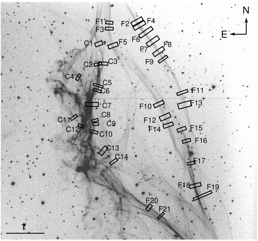
Figure 1.— August 2003 MDM 2.4m H$\alpha$ image of the southwest cloud in the Cygnus Loop showing the location of our selected filaments.

Figure 2.— Left: One-dimensional shock profiles (top) and cross-correlation function(bottom) for region F14. The star appearing in the 1992 data (top, extreme left) is the result of using a wider filter during the 1992 observations. Right: Cloud-shock profile (top) and cross-correlation function (bottom) for region C9.

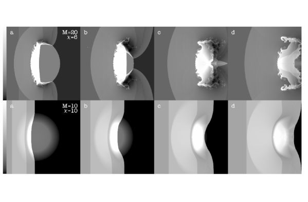
Figure 3.— Density plots of Model 1 (top) and Model 2 (bottom). Model 1 is shown at $t$ = 1.4, 2.6, 3.6, and 4.6 $\times$ 10^-2. Model 2 is shown at $t$ = 3.7, 5,5, 6.9 and 8.2 $\times$ 10^-2.

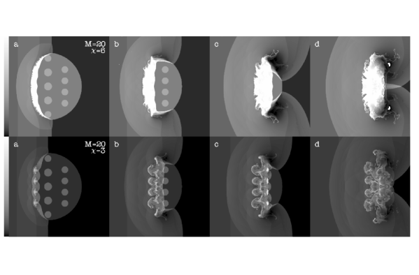
Figure 4.— Same as Figure 3 for Model 3 (top) and Model 4 (bottom). Model 3 is shown at 1.8, 2.9, 4.0, and 4.7 $\times$ 10^-2. Model 4 is shown at 1.7, 3.0, 3.3, and 4.3 $\times$ 10^-2.

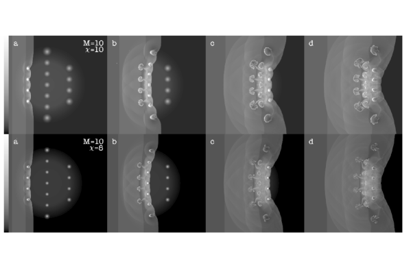
Figure 5.— Same as Figure 3 for Model 5 (top) and Model 6 (bottom). Model 5 is shown at 2.3, 4.6, 6.6, and 7.5 $\times$ 10^-2. Model 6 is shown at 2.3, 4.3, 6.4, and 7.4 $\times$ 10^-2.

References

- Blair et al. (1999) Blair, W. P., Sankrit, R., Raymond, J. C., & Long, K. S. 1999, AJ, 118, 942
- Blair et al. (2005) Blair, W. P., Sankrit, R., & Raymond, J. C. 1999, AJ, 129, 2268
- Blondin & Knerr (1992) Blondin, J. M., & Knerr, J. M. 1992, Bulletin of the American Astronomical Society, 24, 1227
- Colella, & Woodward (1984) Colella, P., & Woodward, P. R. 1984, J. Comp. Phys., 54, 174
- DeNoyer (1975) DeNoyer, L. K. 1975, ApJ, 196, 479
- Fesen, Blair, & Kirshner (1982) Fesen, R. A., Blair, W. P., & Kirshner, R. P. 1982, ApJ, 262, 171 ApJS, 118, 541
- Fragile et al. (2004) Fragile, P. C., Murray, S. D., Anninos, P., & van Breugel, W. 2004, ApJ, 604, 74
- Fragile et al. (2005) Fragile, P. C., Anninos, P., Gustafson, K., & Murray, S. D. 2005, ApJ, 619, 327
- Kahn (1976) Kahn, F. D. 1976, A&A, 50, 145
- Klein, McKee, & Colella (1994) Klein, R. I., McKee, C. F., & Colella, P. 1994, ApJ, 420, 213
- Levenson & Graham (2001) Levenson, N. A. & Graham, J. R. 2001, ApJ, 559, 948
- Mac Low et al. (1994) Mac Low, M., McKee, C. F., Klein, R. I., Stone, J. M., & Norman, M. L. 1994, ApJ, 433, 757
- Mellema et al. (2002) Mellema, G., Kurk, J. D., Rottgering, H. J. A. 2002, A&A, 395, L13
- Nittman, Falle, & Gaskell (1982) Nittman, J., Falle, S., P. H. 1982, MNRAS, 201, 833
- Parker (1967) Parker, R. A. R. 1967, ApJ, 149, 363
- Patnaude et al. (2002) Patnaude, D. J., Fesen, R. A., Raymond, J. C., Levenson, N. A., Graham, J. R., & Wallace, D. J. 2002, AJ, 124, 2118
- Poludnenko, Frank, & Blackman (2002) Poludnenko, A. Y., Frank, A., & Blackman, E. G. 2002, ApJ, 576, 832
- Stevens et al. (1992) Stevens, I. R., Blondin, J. M., & Pollock, A. M. T. 1992, ApJ, 386, 265
- Stone & Norman (1992) Stone, J. M., & Norman, M. L. 1992, ApJ, 390, L17
- Tonry & Davis (1979) Tonry, J. and Davis, M. 1979, AJ, 84, 1511
- Thorstensen, Fesen, & van den Bergh (2001) Thorstensen, J. R., Fesen, R. A., & van den Bergh, S. 2001, AJ, 122, 297
- Woodward (1976) Woodward, P. R. 1976, ApJ, 207, 484