The subpulse modulation properties of pulsars at 21 cm

We present the results of a systematic, unbiased search for subpulse modulation of 187 pulsars performed with the Westerbork Synthesis Radio Telescope (WSRT) in the Netherlands at an observing wavelength of 21 cm. Using new observations and archival WSRT data we have expanded the list of pulsars which show the drifting subpulse phenomenon by 42, indicating that at least one in three pulsars exhibits this phenomenon. The real fraction of pulsars which show the drifting phenomenon is likely to be larger than some 55%. The majority of the analysed pulsars show subpulse modulation (170), of which the majority were not previously known to show subpulse modulation and 30 show clear systematic drifting. The large number of new drifters we have found allows us, for the first time, to do meaningful statistics on the drifting phenomenon. We find that the drifting phenomenon is correlated with the pulsar age such that drifting is more likely to occur in older pulsars. Pulsars which drift more coherently seem to be older and have a lower modulation index. There is no significant correlation found between $P_{3}$ and other pulsar parameters (such as the pulsar age), as has been reported in the past. There is no significant preference of drift direction and the drift direction is not found to be correlated with pulsar parameters. None of the four complexity parameters predicted by different emission models (Jenet & Gil 2003) are shown to be inconsistent with the set of modulation indices of our sample of pulsars. Therefore none of the models can be ruled out based on our observations. We also present results on some interesting new individual sources like a pulsar which shows similar subpulse modulation in both the main- and interpulse and six pulsars with opposite drift senses in different components.

1 Introduction

Despite the fact that explaining the emission mechanism of radio pulsars has proved very difficult, this field has the advantage that we have very detailed knowledge about the emission mechanism from observations. We know from the very high observed brightness temperatures that the radio emission must be coherent, we know what kind of magnetic field strengths are involved and even the orientation of the magnetic axis, rotation axis and the line of sight can be derived from observations. Furthermore if one can detect single pulses one can see that the pulses of some pulsars consist of subpulses and for some pulsars these subpulses drift in successive pulses in an organized fashion through the pulse window (Drake & Craft 1968; Sutton et al. 1970). If one plots a so-called “pulse-stack”, a plot in which successive pulses are displayed on top of one another, the drifting phenomenon causes the subpulses to form “drift bands” (an example is shown in the left panel of Fig. 1). This complex, but highly regular intensity modulation in time is known in great detail for only a small number of well studied pulsars.

Because the properties of the subpulses are most likely determined by the emission mechanism, we learn about the physics of the emission mechanism by studying them. That drifting is linked with the emission mechanism is suggested by the fact that drifting is affected by “nulls” (e.g. Taylor & Huguenin 1971; van Leeuwen et al. 2002; Janssen & van Leeuwen 2004), where nulling is the phenomenon whereby the emission mechanism is switched off for a number of successive pulses. Another complex phenomenon is drift mode changes where the drift rate switches between a number of discrete values. For some pulsars there are observationally determined rules describing which drift mode changes are allowed from which drift mode (e.g. Wright & Fowler 1981; Redman et al. 2005). It has been found that the nulls of PSR B2303+30 are confined to a particular drift mode (Redman et al. 2005), which further strengthens the link between drifting and the emission mechanism.

Another characteristic feature of the emission mechanism is that when one averages the individual pulses, the resulting pulse profile is remarkably stable over time (Helfand et al. 1975). Explaining the various shapes of the pulse profiles of different pulsars and their dependence on observing frequency has proven to be very complicated, so not surprisingly an explanation that is fully consistent with the overwhelmingly detailed complex behavior of individual (sub)pulses, the nulling phenomenon and the polarization of individual pulses (e.g. Edwards 2004) seems to be far away. In this paper we describe trends of the subpulse modulation we find for a large sample of pulsars. By doing this we determine observationally what the important physical parameters are for subpulse modulation, which could help formulating an emission model which is fully consistent with the observations.

There are a few types of models that attempt to explain the drifting phenomenon. The most well known model is the sparking gap model (Ruderman & Sutherland 1975), which has been extended by many authors (e.g. Cheng & Ruderman 1980; Filippenko & Radhakrishnan 1982; Gil & Sendyk 2000; Gil et al. 2003; Qiao et al. 2004) making it the most developed model for explaining the drifting phenomenon. These models explain the drifting phenomenon by the generation of the radio emission via a rotating “carousel” of discharges which circulate around the magnetic axis due to an $\mathbf{E}\times\mathbf{B}$ drift. In the carousel model it is expected that all pulsars should have some sort of circulation time. For PSR B0943+10 (Deshpande & Rankin 1999, 2001; Asgekar & Deshpande 2001) and possibly PSR B0834+06 (Asgekar & Deshpande 2005) a tertiary subpulse modulation feature has been detected from the fluctuation properties and viewing geometry. This periodicity has been interpreted as related to the carousel modulation period (i.e. the circulation time $\hat{P}_{3}$), supporting the interpretation of the drifting subpulses being caused by a rotating carousel of sub-beams. The circulation times of these pulsars, as well as the more indirectly derived circulation times of PSR B0809+74 (van Leeuwen et al. 2003) and PSR B0826$-$34 (Gupta et al. 2004) are consistent with the sparking gap model (Gil et al. 2003). A different geometry of the polar cap of PSR B0826$-$34 is proposed by Esamdin et al. 2005. In their interpretation the carousel changes drift direction, something what would be inconsistent with the sparking gap model.

These models still have problems, like explaining the subpulse phase steps which are observed for some pulsars. Two clear examples of pulsars that show subpulse phase steps are PSR B0320+39 and PSR B0809+74 as found by Edwards et al. (2003) and Edwards & Stappers (2003b). We find that the new drifter PSR B2255+58 also shows a phase step.

Non-radial pulsations of neutron stars were originally proposed as the origin of the radio pulses of pulsars (Ruderman 1968) and later as a possible origin of the drifting subpulses (Drake & Craft 1968). Recently this idea was revised by Clemens & Rosen (2004). This model gives a natural explanation for observed subpulse phase steps, nulls and mode changes. This model can be tested, although there are many complications, by exploring average beam geometries. Although this model can explain phase steps, it cannot explain the curvature of the drift bands of many pulsars (see Sect. 4.5 for details). In this model it is also difficult to explain pulsars with opposite drift senses in different components, because drifting is a simply a beat between the pulse period and the pulsation time. Bi-drifting is recently observed for PSR J0815+09 (McLaughlin et al. 2004). In this paper we show a number of other pulsars with opposite drift senses in different components. For PSR B1839$-$04 we observe that the two components have mirrored drift bands (i.e. the components drift in phase) like PSR J0815+09, something we do not know for the other pulsars. In the sparking gap model bi-drifting can be explained if these pulsars have both an inner annular gap and an inner core gap (Qiao et al. 2004).

A feedback model is proposed by Wright (2003) as a natural mechanism for both the sometimes regular and sometimes chaotic appearance of subpulse patterns. In this model the outer magnetosphere interacts with the polar cap and the observed dependency of conal type on pulse period (Rankin 1993a) and angle between the rotation and magnetic axis (Rankin 1990) follows naturally.

Up to now most observational literature on the drifting phenomenon has been focused on describing individual very interesting drifting subpulse pulsars. The focus of this paper will not only be the individual systems, but also the properties common to the pulsars that show drifting, an approach started by Backus (1981), Ashworth (1982) and Rankin (1986). In the work of Backus (1981) 20 pulsars were studied for their subpulse behavior at 430 MHz and 9 were observed to be drifting. In the work of Ashworth (1982) the single pulse properties of nine new drifters are described and the properties common to 28 drifters in a sample of 52 pulsars are analysed. This sample consists of both their own results and a few previously published results. Most observations were obtained at or near 400 MHz, but some at higher frequencies.

In the work of Rankin (1986) all the, then published, single pulse properties are combined and described in the light of her empirical theory. Because understanding the drifting phenomenon is considered important for unraveling the mysteries of the emission mechanism of radio pulsars, we decided that it was time to start this more general and extensive observational program on the drifting phenomenon.

The main goals of this unbiased search for pulsar subpulse modulation is to determine what percentage of the pulsars show the drifting phenomenon and to find out if these drifters share some physical properties. As a bonus of this observational program new individually interesting drifting subpulse systems are found. In this paper we focus on the 21 cm observations and in a subsequent paper we will focus on lower frequency observations and the frequency dependence of the subpulse modulation properties of radio pulsars.

The list of pulsars which show the drifting phenomenon is slowly expanding in time as more sufficiently bright pulsars are found by surveys (e.g. Lewandowski et al. 2004), but we have successfully chosen a different approach to expand this list much more rapidly. The reason that we have found so many new drifting subpulse systems is twofold: we have analyzed a large sample of pulsars of which many were not known to show this phenomenon, and we used a sensitive detection method. Previous studies of drifting subpulses often used tracking of individual subpulses through time, an analysis method that requires a high signal-to-noise (S/N) ratio because it requires the detection of single pulses. This automatically implies that this kind of analysis can only be carried out on a limited number of pulsars. Analyzing the integrated Two-Dimensional Fluctuation Spectrum (2DFS; Edwards & Stappers 2002) and the Longitude-Resolved Fluctuation Spectrum (LRFS; Backer 1970) allows us to detect drifting subpulses even when the S/N is too low to see single pulses. This method was already successfully used with archival Westerbork Synthesis Radio Telescope (WSRT) data by Edwards & Stappers (2003a) to find drifting subpulses in millisecond pulsars.

By using the technique described above combined with the high sensitivity of the WSRT we have analyzed a large sample of 187 pulsars. An important aspect when calculating the statistics of drifting is that one has to be as unbiased as possible, so we have selected our sample of pulsars based only on the predicted S/N in a reasonable observing time. While this sample is obviously still luminosity biased, it is not biased towards well-studied pulsars, pulse profile morphology or any particular pulsar characteristics as were previous studies (e.g. Ashworth 1982, Backus 1981 and Rankin 1986 and references therein). Moreover, all the conclusions in this paper are based on observations at a single frequency.

The paper is organized such that we start by explaining the technical details of the observations and data analysis. After that the details of the individual detections are described and in table The subpulse modulation properties of pulsars at 21 cm all the details of our measurements can be found. After the individual detections the statistics of the drifting phenomenon are discussed followed by the summary and conclusions. In appendix A are the plots for all the pulsars in our source list. They can also be found in appendix B, but there they are ordered by appearance in the text. Note that the astro-ph version is missing the appendices due to file size restrictions. Please download appendices from http://www.science.uva.nl/$\sim$wltvrede/21cm.pdf.

2 Observations and data analysis

2.1 Source list

All the analyzed observations were collected with the WSRT in the Netherlands. The telescope is located at a latitude of $52^{\circ}$.9 in the north, meaning that not all pulsars are visible for the WSRT. Only catalogued pulsars with a declination (J2000) above -$30^{\circ}$ were included in our source list.

This list of pulsars that are visible to the WSRT was sorted on the observation duration required to achieve a signal-to-noise (S/N) ratio of 130. Of this list we selected the first 191 pulsars, which required observations less then half an hour in duration. The S/N ratio of a pulsar observation can be predicted with the following equation (Dewey et al. 1985)

$$\mathrm{S/N}=\frac{\eta_{Q}SG}{T_{\mathrm{sys}}+T_{\mathrm{sky}}}\sqrt{\frac{\Delta\nu\,t_{\mathrm{obs}}n_{p}(P_{0}-w)}{w}}$$ (1)

where $\eta_{Q}$ is the digitization efficiency factor, $S$ the mean flux density of the pulsar, $G$ the gain of the telescope, $T_{\mathrm{sys}}$ the system temperature, $T_{\mathrm{sky}}$ the sky temperature, $\Delta\nu$ the bandwidth of the pulsar backend, $t_{\mathrm{obs}}$ the observation duration, $n_{p}$ the number of polarizations that are recorded, $P_{0}$ the barycentric pulse period of the pulsar and $w$ the width of the pulse profile.

All observations were conducted with the 21 cm backend at WSRT, which has the following receiver system parameters: $\eta_{Q}=1$, $G=1.2$ K/Jy, $T_{\mathrm{sys}}=27$ K, $T_{\mathrm{sky}}=6$ K (which is the average of the entire sky), $\Delta\nu=80$ MHz and $n_{p}=2$. It is required that the pulsars have an integrated pulse profile with a predicted S/N ratio of 130, so the required observation duration in seconds is

$$t_{\mathrm{obs}}\geq\left(\frac{283\;\mathrm{mJy}}{S_{1400}}\right)^{2}\frac{w}{P_{0}-w}$$ (2)

where $S_{1400}$ is the flux of the pulsar at our observation frequency of 1400 MHz and $w$ the FWHM of the pulse profile. Those pulsars lacking the necessary parameters ($S_{1400}$ and $w$) in the catalog were excluded from the sample, because in such cases it was not possible to evaluate $t_{\mathrm{obs}}$.

The sensitivity to detect drifting subpulses does not only depend on the S/N ratio of the observation, but also on obtaining a large number of pulses. This is because the observation should contain enough drift bands to be able to identify the drifting phenomenon. Our second requirement on the minimum observation length was therefore that the observations should contain at least one thousand pulses, so some pulsars had to be observed for longer than was required to get a S/N ratio of 130. To make sure that the statistics on the drifting phenomenon is not biased on pulse period, it is important to include these long period pulsars in the source list.

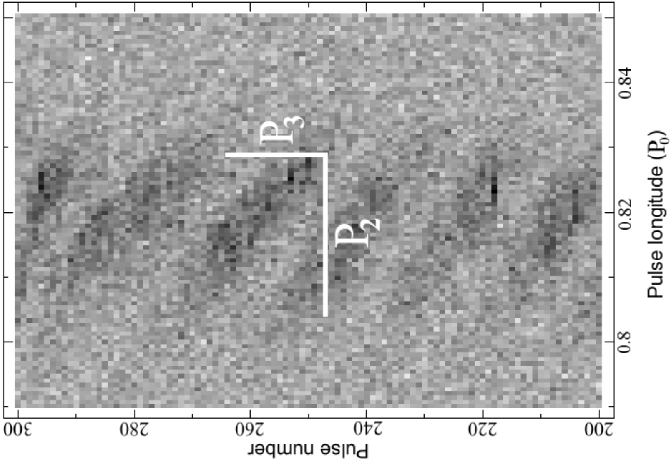
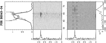
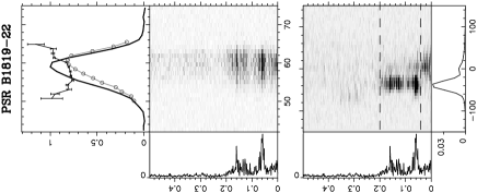
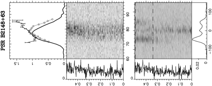
Figure 1: The left panel shows a pulse-stack of one hundred successive pulses of PSR B1819$-$22. Two successive drift bands are vertically separated by $P_{3}$ and horizontally by $P_{2}$. The products of our analysis are shown for three pulsars. The top panel shows the integrated pulse profile (solid line), the longitude-resolved modulation index (solid line with error bars) and the longitude-resolved standard deviation (open circles). Below this panel the LRFS is shown with on its horizontal axis the pulse longitude in degrees, which is also the scale for the abscissa of the plot above. Below the LRFS the 2DFS is plotted and the power in the 2DFS is vertically integrated between the dashed lines, producing the bottom plots. Both the LRFS and 2DFS are horizontally integrated, producing the side-panels of the spectra. See the main text for further details about the plots.

Archival data was used if available and the sample of pulsars was completed with new observations. The best WSRT data available was chosen, so for a number of pulsars the data greatly exceed the minimum S/N and the number of pulses requirement. This does not bias our sample of observations toward well-studied pulsars, because all the observations are long enough to provide a good chance to detect the drifting phenomenon. We have observations of all the sources except the millisecond pulsar B1821$-$24, because of the high time resolution required and the associated data storage problems. The observations of PSR B1823$-$13, B1834$-$06 and J1835$-$1020 failed, and therefore are not included in this paper.

2.2 Calculation of the pulse-stacks

All the observations presented in this paper were made at an observation wavelength of 21 cm spread out over the last five years. The signals of all fourteen 25-meter dishes of the WSRT were added together by taking into account the relative time delays between them and processed by the PuMa pulsar backend (Voûte et al. 2002). In order to reduce the effects of interference, badly affected frequency channels were excluded. The frequency channels were then added together in an offline procedure after dedispersing them by using previously published dispersion measures.

To study the single pulse behavior of pulsars one usually converts the one-dimensional de-dispersed time series into a two-dimensional pulse longitude versus pulse number array (pulse-stack). An example is shown in the left panel of Fig. 1, where one hundred successive pulses are plotted on top of one other. The pulse number is plotted vertically and the time within the pulses (i.e. the pulse longitude) horizontally. The off-pulse region is used to remove the baseline from the pulsar signal, making the average noise level zero.

To correct for the pulse longitude shift of successive pulses the TEMPO software package was used. Because the pulse period ($P_{0}$) of the pulsar is not exactly equal to an integer number of time sample intervals, each pulse (as it appears in the binned sequence) is effectively shifted by a constant amount modulo one bin. This induces, as noted by Vivekanand et al. 1998, a periodic longitude shift of successive pulses. Following Edwards & Stappers (2003a), we have compensated for this longitude shift of each pulse, and thereby avoiding artificial features appearing in the spectra that are derived from the pulse-stacks. All pulse longitudes in this paper have an arbitrary offset because absolute alignment was not necessary for our analysis.

In the left panel of Fig. 1 one can see a sequence of 100 pulses of one of the new drifters we have found which clearly shows the drifting phenomenon. Drifting means that the subpulses drift in longitude from pulse to pulse and thereby the pulsar emission shows diagonal intensity bands in the pulse-stack (drift bands). The drift bands are characterized by two numbers: the horizontal separation between them in pulse longitude ($P_{2}$) and the vertical separation in pulse periods ($P_{3}$). The drift bands of this pulsar are clearly seen by eye in the pulse-stack and the values $P_{2}$ and $P_{3}$ could in principle be measured directly, but in many cases of the newly discovered drifters the drift bands are not visible to the eye. To be able to detect the drifting phenomenon in as many pulsars as possible, all the pulse-stacks were analyzed in a systematic way as described in the next two subsections.

2.3 Processing of the pulse-stacks

In Fig. 1 the products of our method of analysis are shown for three pulsars and in this section it is explained how these plots are generated from the pulse-stack and how one can interpret them.

The first thing that is produced from the pulse-stack is the integrated pulse profile. This is simply done by vertically integrating the pulse-stack, i.e. adding the bins with the same pulse longitude in the successive pulses:

$$\mu_{i}=\frac{1}{N}\sum_{j=0}^{N-1}S_{ij}$$ (3)

Here $\mu_{i}$ is the average intensity at longitude bin $i$, and $S_{ij}$ is the signal at pulse longitude bin $i$ and pulse number $j$ in the pulse-stack and $N$ is the number of pulses. In Fig. 1 the solid line in the top panels corresponds to the integrated pulse profile $\mu_{i}$ (which is normalized to the peak intensity). On the horizontal axis is the pulse longitude in degrees and the value can be read from the horizontal axis of the panel below which is aligned with the top panel.

The first basic method to find out if there is some kind of subpulse modulation is to calculate the longitude-resolved variance $\sigma^{2}_{i}$

$$\sigma^{2}_{i}=\frac{1}{N}\sum_{j=0}^{N-1}(S_{ij}-\mu_{i})^{2}$$ (4)

and the longitude-resolved modulation index $m_{i}$

$$m_{i}=\frac{\sigma_{i}}{\mu_{i}}$$ (5)

The modulation index is a measure of the factor by which the intensity varies from pulse to pulse and could therefore be an indication for the presence of subpulses. In Fig. 1 the open circles in the top panel is the longitude-resolved standard deviation $\sigma_{i}$ and the solid line with error bars corresponds to the longitude-resolved modulation index $m_{i}$.

The detection of a modulation index does not give information about whether the subpulse modulation occurs in a systematic or a disordered fashion. The first step in detecting a regular intensity variation is to calculate the Longitude Resolved Fluctuation Spectrum (LRFS; Backer 1970). The pulse-stack is divided into blocks of 512 successive pulses and the Discrete Fourier Transform (DFT) was performed on these blocks to calculate the LRFS (for details of the analysis we refer to Edwards & Stappers 2002, 2003a). The fluctuation power spectra of the different blocks were then averaged to obtain the final spectrum.

In Fig. 1 the LRFS of the three pulsars are shown below the pulse profile plots. The units of the vertical axis are in cycles per period (cpp), which corresponds to $P_{0}/P_{3}$ in the case of drifting (where $P_{3}$ is the vertical drift band separation). The horizontal axis is the pulse longitude in degrees, which is aligned with the plot above. The power in the LRFS is horizontally integrated, producing the side panel. If the emission of the pulsar is modulated with a period $P_{3}$, then a distinct region of the LRFS will show an excess of power (i.e. a feature) in the corresponding pulse longitude range. The LRFS can be used to see at which pulse longitudes the pulsar shows subpulse modulation and with which periodicities. The grayscale in the LRFS corresponds to the power spectral density. Under Parseval’s theorem, the summed LRFS is identical to Eq. 4 (Edwards & Stappers 2003a), so integrating the LRFS vertically gives the longitude resolved variance (the open dots in the plot above the LRFS).

The detection of a modulation index suggests that there is subpulse modulation and by analyzing the LRFS it can be determined if this modulation is disordered or (quasi-)periodic. However from the LRFS one cannot determine if the subpulses are drifting over a certain longitude range, because to calculate the LRFS only DFTs along vertical lines in the pulse-stack are performed. To determine if the subpulses are drifting, the Two-Dimensional Fluctuation Spectrum (2DFS; Edwards & Stappers 2002) is calculated. The procedure is similar to calculating the LRFS, but now we select one or more pulse longitude ranges between which the DFT is not only calculated along vertical lines, but along lines with various slopes. The effect is that the pulse longitude information that we had in the LRFS is lost, but we gain the sensitivity to detect periodic subpulse modulation in the horizontal direction (i.e. if there also exists a preferred $P_{2}$ value). Following the same procedure used while calculating the LRFS, the pulse-stack is divided in blocks of 512 successive pulses and the spectra of the different blocks were then averaged to obtain the final spectra.

In Fig. 1 the 2DFS is plotted below the LRFS. The vertical axis has the same units as the LRFS, but now the units of the horizontal axis are also cycles per period, which corresponds to $P_{0}/P_{2}$ in the case of drifting (where $P_{2}$ is the horizontal drift band separation in time units). The power in the 2DFS is horizontally and (between the dashed lines) vertically integrated, producing the side and bottom panels in Fig. 1. These panels are only produced to make it easier to see by eye what the structure of the feature is.

From the pulse-stack in Fig. 1 one can see that two successive drift bands of PSR B1819$-$22 are vertically separated by $P_{3}\approx 18.0P_{0}$ and horizontally by $P_{2}\approx 0.025P_{0}$. Instead of measuring drifting directly from the pulse-stack, we use the 2DFS. From both the 2DFS and LRFS of this pulsar we see that there are multiple drift features. This is because PSR B1819$-$22 is a drift mode changer (i.e. the drift bands have different slopes in different parts of the observation). We note that only one drift mode is seen in the short stretch of pulses shown in the pulse-stack in Fig. 1. For PSR B1819$-$22 one can see the main feature in the LRFS around 0.056 cpp, which corresponds to the $P_{3}$ value we see in the plotted pulse-stack. In the 2DFS of this pulsar we see the main feature at the same vertical position as in the LRFS (corresponding to the same $P_{3}$ value) and because the feature is offset from the vertical axis we know that the subpulses drift. From the horizontal position of the feature in the 2DFS we see that $P_{2}\approx-P_{0}/40=-0.025P_{0}$, which corresponds well with the $P_{2}$ measured directly from the pulse-stack shown.

In this paper we use the convention that $P_{3}$ is always a positive number and $P_{2}$ can be either positive or negative. A negative value of $P_{2}$ means that the subpulses appear earlier in successive pulses, which is called negative drifting in the literature. The tabulated signs of $P_{2}$ in this paper therefore correspond to the drift direction, such that a positive sign corresponds to positive drifting. To comply with this convention, all the plotted 2DFSs in this paper are in fact flipped about the vertical axis compared with the definition of the 2DFS in Edwards & Stappers (2002).

2.3.1 Interference

To reduce the effect of interference on the LRFS and 2DFS the spectrum of the off-pulse noise was subtracted from the LRFS and 2DFS if a large enough off-pulse longitude interval was available. Interference will in general not be perfectly removed by this procedure, however any artificial features produced by interference can easily be identified because it will not be confined to a specific pulse longitude range. In Fig. 1 the spectra of PSR B2043$-$04 shows interference with a $P_{0}/P_{3}\simeq 0.372$. In the spectra as shown in appendix A and B, the channels containing interference are set to zero, thereby improving the visual contrast of the plots.

In this paper the modulation index is not directly derived from the pulse-stack (Eqs. 4 and 5), but from the LRFS. This is done by vertically integrating the LRFS, which gives the longitude resolved variance (Eq. 4). The advantage of this method is that by excluding the lowest frequency bin the effect of interstellar scintillation (which at this observing frequency has typical low frequencies) can be removed from the modulation index (for details of the analysis we refer to Edwards & Stappers 2002, 2003a). After exclusion of the lowest frequency bins the variance is overestimated by $m^{2}_{\mathrm{scint}}$, where $m^{2}_{\mathrm{scint}}$ is the modulation index induced by the scintillation (see Eqs. 20-22 of Edwards & Stappers 2004). The longitude resolved modulation index and standard deviation are corrected accordingly.

2.4 Analysis of the drift features

If a feature is seen in the 2DFS and we make sure it is not associated with interference, $P_{2}$ and $P_{3}$ can be measured and its significance determined. The drift feature will always be smeared out over a region in the 2DFS. This could be because there is not one fixed value of the drift rate throughout the observation due to random slope variations of the drift bands, drift mode changes or nulling. But the feature is also broadened if the drifting is not linear (i.e. subpulse phase steps or swings) and because of subpulse amplitude windowing (Edwards & Stappers 2002).

Because of all these effects it is impossible to fit one specific mathematical function to all the detected features, so it is more practical to calculate the centroid of a rectangular region in the 2DFS containing the feature. The advantage of this procedure is that no particular shape of the feature has to be assumed. The centroids are defined as:

$$P_{0}/P_{3} = \frac{1}{F}\sum_{k,l}y_{l}F_{kl}$$

$$P_{0}/P_{2} = \frac{1}{F}\sum_{k,l}x_{k}F_{kl}$$ (6)

Here $k$ and $l$ are indices for the horizontal and vertical position within the region in the 2DFS containing the feature, $x_{k}$ and $y_{l}$ are the corresponding axis values of bin $(k,l)$, $F_{kl}$ is the power in that bin and $F=\sum_{k,l}F_{kl}$ is the total power in the selected region of the 2DFS. An uncertainty on the position of the centroid (hence on $P_{2}$ and $P_{3}$) can be estimated by using the power in a region in the 2DFS that only contains noise. However we have found that in most cases the uncertainty is dominated by the more or less arbitrary choice of what exact region in the 2DFS is selected around the feature. To estimate this uncertainty we have therefore calculated the centroid for slightly different regions containing the feature.

Because the analyzed pulse sequences are sometimes relatively short, there is the possibility that the occasional occurrence of strong (sub)pulses are dominating the spectra and therefore lead to misleading conclusions. To estimate what kind of “random” fluctuation features one can expect from a given pulse sequence, we have randomized the order of the pulses and then passed this new pulse-stack through our software to determine the magnitude of any features which could be attributed to strong (sub)pulses. Any actual drifting will lose coherence in this process and thus we can use the randomized results when estimating the significance of drift features when there is no well defined $P_{3}$.

For most pulsars there is power along the vertical axis in the 2DFS. Therefore the centroid of a larger region around a drift feature usually results in a centroid located closer to the vertical axis, hence in a larger absolute value of $P_{2}$. In most cases this causes the uncertainty on $P_{2}$ to be asymmetric around its most likely value and therefore it is useful to tabulate the uncertainty in both signs.

If the centroid of the feature in the 2DFS is significantly offset from the vertical axis, it means that $P_{0}/P_{2}\neq 0$ and that drifting can be associated with the feature (i.e. there exists a preferred drift direction of the subpulses from pulse to pulse). Drifters are defined in this paper as pulsars which have at least one feature in its 2DFS which show a significant finite $P_{2}$. It must be noted that drift bands are often very non-linear and therefore the magnitude of $P_{2}$ is probably of little meaning. Also we want to emphasize that not only an offset from the vertical axis indicates drifting, but any asymmetry about the vertical axis indicates drifting-like behavior. Any frequency dependence along the vertical axis indicates structured subpulse modulation, either quasi-periodic or as a low frequency excess. Pulsars with a low frequency excess show an excess of power in their spectra toward long frequencies (i.e. the spectra are “red”).

The drifters are classified into three classes and an example of each class is shown in Fig. 1. One can see that PSR B2043$-$04 has a vertically narrow drift feature in its spectra, meaning that $P_{3}$ has a stable and fixed value throughout the observation. We will call these pulsars the coherent drifters class (class Coh in table The subpulse modulation properties of pulsars at 21 cm). The criterion used for this class is that the drift feature has a vertical extension smaller than 0.05 cpp. The pulsars that show a vertical, broad, diffuse drift feature are divided into two classes, depending on whether the feature is clearly separated from the alias borders ($P_{0}/P_{3}=0$ and $P_{0}/P_{3}=0.5$). In table The subpulse modulation properties of pulsars at 21 cm the pulsars in class Dif are clearly separated from the alias border and the pulsars in class Dif^∗ not. In Fig. 1 PSR B1819$-$22 is a diffuse (Dif) drifter and PSR B2148+63 is a Dif^∗ drifter.

Besides the drifters there is also a class of pulsars which show longitude stationary subpulse modulation (class Lon in table The subpulse modulation properties of pulsars at 21 cm). These pulsars show subpulse modulation with a $P_{3}$ value, but without a finite $P_{2}$ value. Because it is not clear if these pulsars should be counted as drifters or as non-drifters, they are excluded from the statistics.

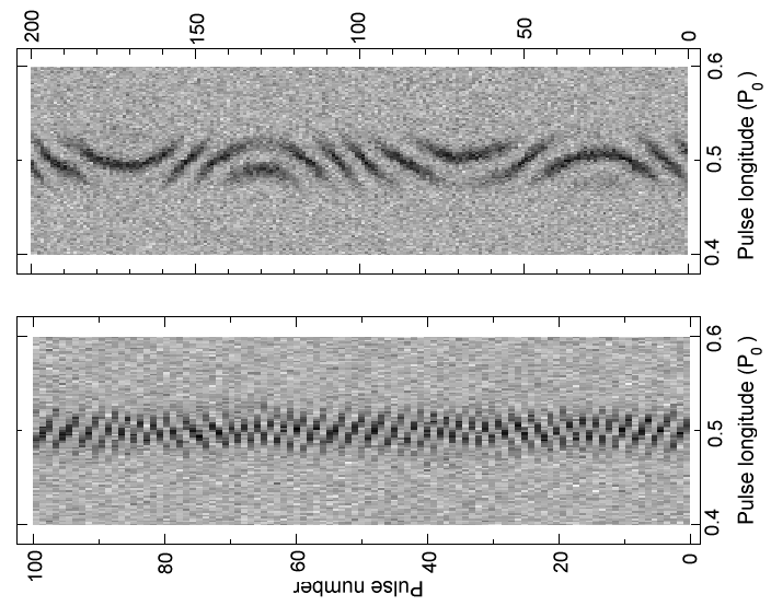
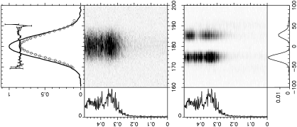
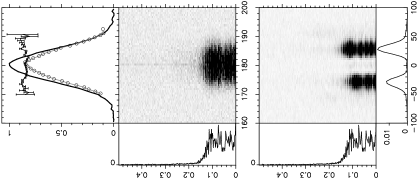
Figure 2: A section of the pulse-stacks and the derived spectra of the two artificially generated pulse sequences to illustrate possible effects of pulsars that constantly change their alias order. The drifting in the left pulse-stack constantly crosses the $P_{3}=2P_{0}$ alias border and the right pulse-stack constantly changes its apparent drift direction via longitude stationary subpulse modulation. For the explanation of the plots we refer to Fig. 1 and the main text.

For many pulsars we find that the magnitude of $P_{2}$ exceeds the pulse width. This means in the case of regular drifting that in a single pulse only one subpulse is visible and that the drifting will manifest itself more as an amplitude modulation rather than as a phase modulation. An illustrative example of a regular drifter with a large $P_{2}$ is PSR B0834+06 (Asgekar & Deshpande 2005). Whether the drifting manifests itself more as an amplitude modulation or as a phase modulation will largely depend on the viewing geometry. Also the presence of pulse sequences without organized drifting, longitude stationary subpulse modulation or drift reversals will result in a large $P_{2}$ value.

It must be noted that the calculation of the 2DFS is an averaging process. This is what makes it a powerful tool to detect drifting subulses in low S/N observations, but at the same time this implies that different pulse-stacks can produce similar 2DFS. For instance a feature that is split and shows a horizontal separation can be caused by drift reversals, but also by subpulse phase steps or swings (see Edwards et al. 2003 for a pulse sequence of PSR B0320+39 and the resulting 2DFS). Note also that with only the LRFS it is impossible to identify complex drift behavior like drift reversals or subpulse phase steps.

The details of each observation can be found in table The subpulse modulation properties of pulsars at 21 cm, including the classification we made, the measured $P_{2}$ and $P_{3}$ values, the modulation index and the detection threshold for the modulation index. It must be emphasized that the $P_{2}$ and $P_{3}$ values are average values during the observation. Especially when the pulsar is a drift mode changer a different observation may lead to different values for $P_{2}$ and $P_{3}$. The plots of all the pulsars can be found in appendix A. For some of the pulsars the 2DFS for two different pulse longitude ranges are shown if useful. The plots of these pulsars come after the plots of the pulsars with only one 2DFS plot. The same plots can also be found in appendix B, but there they are ordered by appearance in the text instead of ordered by name.

2.4.1 Drift reversals

As can be seen from Fig. 1, the subpulses of PSR B1819$-$22 appear to drift toward the leading part of the pulse profile. In the sparking gap model (e.g. Ruderman & Sutherland 1975), every subpulse is associated with one emission entity close to the surface of the star. These entities (the sparks) move around the magnetic axis, causing the subpulses to drift through the pulse window. Because the emission entities are only sampled once per rotation period of the star, it is very difficult to determine if the subpulses in one drift band correspond to the same emission entity for successive pulses. For instance for PSR B1819$-$22 we do not know if the emission entities drift slowly toward the leading part of the pulse profile (not aliased) or faster toward the trailing part of the pulse profile (aliased).

The physical conditions of the pulsar probably determines what the physical drift rate of the emission entities are, rather than the observed (possibly aliased) drift rate. This could already be a serious problem if one wants to correlate physical parameters of pulsars to the observed drift rate of coherent drifters, for which we at least know they stay in the same alias mode. If a feature in the 2DFS is not clearly separated from the alias borders, the power in that feature could consist of drift bands in different alias modes (i.e. the apparent drift direction could be changing constantly during the observation). In that case the measured value of $P_{3}$ using the centroid of the feature is related to the true drift rate of the emission entities in a complicated way, depending on what fraction of the time the pulsar spends in which alias mode. Therefore it is expected that it will be very hard to find a correlation between physical pulsar parameters and the $P_{3}$ values of the pulsars in the Dif^∗ class, so it will be useful to classify the pulsars depending on whether the features in the 2DFS are clearly separated from the alias borders. Inspection of the pulse-stacks with strong enough single pulses reveals that some of the pulsars in the Dif^∗ class change their drift direction during the observation. This is further evidence to indicate the value of considering the Dif and Dif^∗ classes separately.

To illustrate this we have artificially generated two pulse sequences of a pulsar that has a variable rotation period of the emission entities in two different scenarios (see Fig. 2). In both scenarios the emission entities are simulated to drift from the trailing to the leading edge of the pulse profile with a variable drift rate. In the left sequence the vertical drift band separation $P_{3}$ is close to $2P_{0}$ and in the right sequence the $P_{3}$ period is much larger. In the left sequence the subpulses around the first pulse appear to drift toward the leading edge of the pulse profile. As time increases, we speed up the rotation of the emission entities, which causes $P_{3}$ to become smaller. Around pulse number 15 the Nyquist border $P_{3}=2P_{0}$ is reached and the drift pattern becomes a check-board like pattern. As time further increases the emission entities are still speeding up, causing clear drift bands to reappear with an opposite apparent drift direction (around pulse 25). After this the rotation of the emission entities is gradually slowed down to the initial value, causing the drift bands to change apparent drift direction again around pulse 50. The same cycle is repeated for the next pulses. In this simulation the carousel rotation period is set to vary with about 40% around its mean value.

The resulting spectra of this pulse sequence are also shown in Fig. 2. The LRFS shows that the subpulse modulation is extended toward the $P_{3}=2P_{0}$ alias border and the 2DFS shows a feature that is split by the vertical axis, because there are two apparent drift directions in the pulse sequence. As can be seen in the bottom panel, there is more power in the left peak. This corresponds to more power being associated with negative drifting (drifting toward the leading edge of the pulse profile). This is also directly visible in the pulse-stack. A good example of a known pulsar that shows this kind of drift behavior is PSR B2303+30 (e.g. Redman et al. 2005) and its 2DFS (see Fig. 36) indeed shows a very clear double peaked feature.

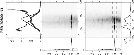
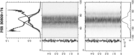
Figure 3: This figure shows the spectra of the well known drifter PSR B0809+74 (left) as well as the results from the same data after putting the pulses in a random order (right).

In the second scenario of Fig. 2 the pulse-stack shows drift bands with a much larger $P_{3}$. Because of possible aliasing this does not directly imply that the emission entities are rotating slower. In fact, we have chosen the entities to rotate faster than in the first scenario. This causes the driftbands to be aliased and the drift bands appear to drift in the opposite direction to the emission entities (which again are simulated to drift toward the leading edge of the pulse profile). As time increases the rotation of the emission entities is sped up. Because of aliasing the drift rate appears to decrease until around pulse 25 the drifting has become longitude stationary ($P_{3}=\infty$). The emission entities are now rotating so fast that in one pulse period time they exactly reappear at the pulse longitude of another drift band. When the rotation period of the emission entities is speeded up even further, the drift bands are changing their apparent drift direction again as can be seen around pulse 50. Now the rotation period of the emission entities is slowed down again until around pulse 100 the initial conditions are reached again. After this the same cycle is repeated. A clear example of a known pulsar that shows this kind of drift reversals is PSR B0826$-$34 (Gupta et al. 2004; Esamdin et al. 2005).

The LRFS of this sequence shows that the subpulse modulation is extended toward the horizontal axis and the 2DFS shows again a feature that is split by the vertical axis. As can be seen in the bottom panel, there is more power in the right peak, which corresponds to more power associated with positive drifting. In the pulse-stack there are indeed more drift bands that drift toward the trailing edge of the pulse profile than in the opposite direction.

2.4.2 Non linear drift bands

In the left panel of Fig. 3 the spectra of the well known regular drifter PSR B0809+74 are shown. The drift feature in the 2DFS shows a clear horizontal structure caused by the non linear drift bands of PSR B0809+74 at this observing frequency (Edwards & Stappers 2003b; Prószyński & Wolszczan 1986; Wolszczan et al. 1981). If drift bands are not straight, there is no one unique value of $P_{2}$ that is associated with the drifting and therefore the drift feature in the 2DFS will be more complex than just one peak. This makes $P_{2}$ an ill-defined parameter. However this is no shortcoming of the 2DFS, it is a shortcoming of the whole concept of $P_{2}$ under curved driftbands. In this paper $P_{2}$ is just a rough measure of the presence of drift, its direction and the magnitude of the slope in a overall mean sense only.

If the drift bands are non linear, the subpulses will have a pulse longitude dependent spacing. This pulse longitude dependent spacing is described by the so-called “modulation phase profile” or “phase envelope” (Edwards & Stappers 2002).

2.4.3 Quasiperiodic subpulses

For most drifters the vertical drift band separation $P_{3}$ is a much better defined parameter than the horizontal separation $P_{2}$, e.g. the drift feature in the 2DFS of PSR B0809+74 (left panel of Fig. 3) is much sharper in the vertical direction than in the horizontal direction. There is however the possibility that single pulses show regular spaced subpulses, while there is no memory for where the subpulses appear in successive pulses. In that case there is a $P_{2}$ value, but $P_{3}$ is undefined. One can simulate such a scenario by putting the pulses of a regular drifter in a random order. This is done for PSR B0809+74 in the right panel of Fig. 3.

One can see, first of all, that the longitude-resolved standard deviation and modulation index are independent on the ordering of the pulses, as expected from Eqs. 4 and 5. Secondly, the spectra do not show any vertical structure anymore. This indicates that, as expected, $P_{3}$ has become undefined. The 2DFS is symmetric about the vertical axis, so there is no preferred drift direction anymore. The horizontal subpulse separation is however still visible in the 2DFS as two vertical bands at $\pm 37$ cpp, the same horizontal position as the largest peak in the 2DFS in the left panel of Fig. 3.

We have found two pulsars that shows these kind of features: PSRs B2217+47 and B0144+59. In the carousel model this phenomenon could be explained by a highly variable circulation time that causes the alias order to change constantly. However there is no evidence that this phenomenon is related to the same origin as the drifting subpulses, as it only shows that the subpulses appear quasiperiodic.

3 Individual detections

3.1 Coherent drifters (class “Coh”)

The coherent drifters are the pulsars which show a drift feature in their 2DFS over a small $P_{3}$ range (smaller than 0.05 cpp). First the pulsars that were already known to have drifting subpulses are described followed by the pulsars that were not known to show this phenomenon.

3.1.1 Known drifters

B0148$-$06: Both components of the pulse profile of this pulsar have the same drift sign and $P_{3}$ varies slightly during the observation (see Fig. 36). The drift bands are clearly visible in the pulse-stack and the drifting is most prominent in the leading component. The feature in the leading component seems to consist of different drift modes. This is all consistent with results reported by Biggs et al. (1985), who discovered the drifting subpulses at 645 MHz.
B0320+39: This pulsar is known to show very regular drifting subpulses (Izvekova et al. 1982), which is confirmed by the very narrow drift feature in our observation (Fig. 36). Izvekova et al. (1993) have shown that drifting at both 102 and 406 MHz occurs in two distinct pulse longitude intervals and that the energy contribution in the drifting subpulses is less at higher frequencies, especially in the leading component. We see that this trend continues at higher frequencies, because the feature is most prominent in the trailing component at 1380 MHz. The drift feature in the 2DFS shows a clear horizontal structure caused by a subpulse phase step in the drift bands (as is also seen for instance for PSR B0809+74 at this frequency). At both 328 MHz and 1380 MHz the drift bands of PSR B0320+39 are known to show a phase step (Edwards et al. 2003 and Edwards & Stappers 2003b respectively). This is the same observation as used by Edwards & Stappers (2003b).
B0809+74: The drift feature in the 2DFS (Fig. 36) shows clearly horizontal structure, which is caused by a phase step of the drifting subpulses. This phase step is only present at high frequencies and is consistent with Wolszczan et al. (1981) at 1.7 Ghz, Prószyński & Wolszczan (1986) at 1420 MHz and Edwards & Stappers (2003b) at 1380 MHz (this is the same data as used by Edwards & Stappers 2003b). The drift rate is affected by nulls (Taylor & Huguenin 1971) and detailed analysis of this phenomenon allowed van Leeuwen et al. (2003) to conclude that the drift is not aliased for this pulsar.
B0818$-$13: This pulsar has a clear drift feature (Fig. 36) that contains almost all power in the 2DFS. The drift feature has a horizontal structure like observed for PSR B0809+74 and PSR B0320+39. From the modulation phase profile it follows that the drift bands make a smooth swing of about $200^{\circ}$ in subpulse phase in the middle of the pulse profile. A decrease of the drift rate in the middle of the pulse profile has been reported at 645 MHz by Biggs et al. (1987) and this effect appears to be more pronounced in our observation at 1380 MHz. The longitude resolved modulation index shows a minimum at the position of the subpulse phase swing (consistent with Biggs et al. 1987), something that is also observed for the phase steps of PSR B0320+39 and B0809+74. The subpulse phase swing is clearly visible in the pulse-stack of this pulsar. This phase swing seems to be related to the complex polarization behavior of the single pulses as observed by Edwards (2004). For this pulsar nulling was shown to interact with the drift rate by Lyne & Ashworth (1983) and from detailed analysis of this phenomenon Janssen & van Leeuwen (2004) concluded that the drift of this pulsar is aliased.
B1540$-$06: The 2DFS of the two halves of the pulse profile show opposite drift directions (Fig. 36). The drift sense of the leading part of the pulse profile is consistent with the positive drifting of this pulsar as has been reported by Ashworth (1982) at 400 MHz.
B2045$-$16: Only the 2DFS of the trailing component is plotted in Fig. 36, because we do not detect any features in the leading component. However, drifting has been observed previously in both components (e.g. Oster & Sieber 1977) and is observed to be broad with $P_{3}$ values between 2 and 3$P_{0}$ (Oster & Sieber 1977 at 1720 MHz, Nowakowski et al. 1982 at at 1.4 and 2.7 GHz and Taylor & Huguenin 1971 at low frequencies). The second component in our observation has a clear narrow drift feature. This could indicate that this pulsar is a drift mode changer and that our observation was too short to detect the drift rate variations.
B2303+30: This pulsar is known to drift close to the alias border (e.g. Sieber & Oster 1975 at 430 MHz). This pulsar has a clear double-peaked feature in its 2DFS exactly at the alias border (Fig. 36), which suggest that the apparent drift sense changes during the observation because the alias changes during the observation. The change of drift sense can be seen by eye in the pulse-stack and also in the pulse-stacks shown in Redman et al. (2005). These authors show that, besides this $P_{3}\!\!\approx\!\!2P_{0}$ ‘$B$’ drift mode, there is occasionally also a $P_{3}\!\!\approx\!\!3P_{0}$ ‘$Q$’ drift mode if the S/N conditions are good. There is no evidence for this weaker ‘$Q$’-mode in our observation.
B2310+42: The two components of this pulsar are clearly drifting at the alias border (Fig. 36). The drift feature in the trailing component is clearly double peaked, so the alias mode is probably changing during the observation. The leading component shows the same feature at the alias border, although much weaker. The dominant drift sense is consistent with the positive drifting found by Ashworth (1982) at 400 MHz. We also find that the low frequency excess of the leading component is clearly drifting with two signs as well ($P_{2}=65^{\circ}\pm 35$, $P_{3}=21\pm 3P_{0}$ and $P_{2}=-65^{\circ}\pm 15$, $P_{3}=70\pm 10P_{0}$), but no significant drift is detected in the low frequency excess of the trailing component.
B2319+60: This pulsar shows a clear drift component in the 2DFS of the trailing component of the pulse profile and a less clear drift component in the leading component (Fig. 36). No significant drifting is detected in the 2DFS of the center part of the pulse profile (which is not plotted). It has been found that this pulsar is a drift mode changer and that the allowed drift mode transitions follow certain rules (Wright & Fowler 1981 at 1415 MHz). In the 2DFS there is only evidence for one stable drift mode, but drifting is detected over the whole $P_{3}$ range. Drift mode changes can been seen in the pulse-stack. The drift mode we see in the 2DFS is the ‘$A$’ drift mode, which was found by Wright & Fowler (1981) to be the most common drift mode. The many nulls in the pulse-stack probably smears out the feature over a large $P_{3}$ range. There is a sharp $P_{3}\simeq 130P_{0}$ feature in the second component, which could be related to nulling or mode changes.

3.1.2 New drifters (class “Coh”)

B0149$-$16: The 2DFS of this pulsar (Fig. 36) shows a weak drift feature.
B0609+37: Almost all power in the 2DFS of this pulsar is in a well confined drifting feature (Fig. 36), meaning that the subpulse drifting is very organized and stable.
B0621$-$04: A strong and very coherent $P_{3}\simeq 2P_{0}$ feature is seen in the LRFS and 2DFS of this pulsar (Fig. 36), which is also seen in other observations. The feature is significantly offset from the vertical axis, so this pulsar shows very stable drifting subpulses. Only the 2DFS of the trailing peak is plotted.
J1650$-$1654: This pulsar shows a very clear drift feature in its 2DFS (Fig. 36). The feature seems to show some vertical structure, which could be because of drift rate variations. The feature also seems to show some horizontal structure like PSR B0818$-$13, which could indicate that the drift bands are curved or show a phase step. This would be consistent with the minimum in the modulation index in the middle of the pulse profile. However this observation is too short to state if this effect is due to a systematic drift rate change across the pulse profile or due to random variations.
B1702$-$19: The pulse profile of this pulsar shows an interpulse (Biggs et al. 1988). The main pulse shows a drift feature and the 2DFS of the interpulse shows a feature with the same $P_{3}$ value (Fig. 36), but no significant offset from the vertical axis could be detected for this feature. This is not the only pulsar to show correlations in emission properties between the main- and interpulse. PSR B1822$-$09 exhibits an anti-correlation between the intensity in the main- and the interpulse (e.g. Fowler et al. 1981; Fowler & Wright 1982) and also a correlation in the subpulse modulation (e.g. Gil et al. 1994). That pulsar also shows drifting in the main pulse in the ‘$B$’-mode and longitude stationary subpulse modulation in both the main- and interpulse in the ‘$Q$’-mode with the same $P_{3}$. Also PSR B1055$-$52 is known to show a main pulse-interpulse correlation. For that pulsar a correlation between the intensity of the main and interpulse has been found by Biggs (1990). However PSR B1702$-$19 is the first pulsar that shows a correlation between the drifting subpulses in the main pulse and the subpulse modulation in the interpulse.
B1717$-$29: A very narrow drift feature is seen in both the LRFS and the 2DFS of this pulsar (Fig. 36). Because the very low S/N of this observation it was impossible to measure a significant modulation index using the whole $P_{3}$ range of the LRFS. By only using the frequencies in the LRFS that contains the drift feature it was possible to significantly determine the modulation index corresponding to the drift feature. This drifting is confirmed in another observation.
B1839$-$04: Both components of the pulse profile of this pulsar are drifting (Fig. 36). The drift bands are clearly visible in the pulse-stack to the eye and both components have an opposite drift sense. The slope of the drift bands in the two components are mirrored and the drift bands of the two components are also roughly in phase. So when a drift band is visible in one component, it is also visible (although mirrored) in the other component. This “bi-drifting” subpulse behavior is also observed for PSR J0815+09, which also has opposite drift senses in different components (McLaughlin et al. 2004). This “bi-drifting” could be a sign that these pulsars have both an inner annular gap and an inner core gap (Qiao et al. 2004), but also “double imaging” could be responsible (Edwards et al. 2003). Note also that the second harmonic of the drift feature is visible in the 2DFS of especially the trailing component.
B1841$-$04: This pulsar has a weak, definite drift feature in its 2DFS (Fig. 36), which is also visible in the LRFS.
B1844$-$04: There is a weak detection of a narrow drift feature in the 2DFS of this pulsar, which is also visible in the LRFS (Fig. 36).
J1901$-$0906: The trailing component of this pulsar shows a clear and narrow drift feature in its 2DFS, which is not detected in the leading component (Fig. 36). The 2DFS of the leading component has a drift feature with a different $P_{3}$ which is also present in the right component ($P_{2}=-8.2^{\circ}\pm 9.2$, $P_{3}=6.8\pm 0.5P_{0}$). The drifting can be seen by eye in the pulse-stack. The different measured $P_{3}$ values in the two components could indicate that this pulsar is a drift mode changer.
B2000+40: Although this observation is contaminated by interference, clear drifting is detected in the leading component. The rest of the pulse profile (mostly in the trailing component) is also drifting (Fig. 36). The feature in the leading component shows horizontal structure which could be caused by drift reversals or more likely by a subpulse phase jump or swing.
B2043$-$04: This pulsar has a very clear and narrow drifting component in its 2DFS (Fig. 36). The feature is perhaps extended toward the alias border, but this is not significant. Almost all power in the 2DFS is in the drift feature.

3.2 Diffuse drifters (classes “Dif” and “Dif^∗”)

These pulsars show a drift feature over an extended $P_{3}$ range (larger than 0.05 cpp). If the drift feature is clearly separated from both alias borders ($P_{0}/P_{3}=0$ and $P_{0}/P_{3}=0.5$), the pulsar is classified as Dif. However if it is not the pulsar is classified as Dif^∗ in table The subpulse modulation properties of pulsars at 21 cm. In this section the pulsars in the latter class are indicated with an asterisk next to their name. Note that not all drift features in the spectra have peaks which are offset from the vertical axis, but they must be asymmetric about the vertical axis.

3.2.1 Known drifters

B0031$-$07: This pulsar shows a broad drifting feature in its 2DFS (Fig. 36). Three drift modes have been found for this pulsar by Huguenin et al. (1970) at 145 and 400 MHz. In our observation most power in the 2DFS is due to the ‘$A$’-mode drift ($P_{3}=12P_{0}$). The slope of the drift bands change from band to band (e.g. Vivekanand & Joshi 1997), causing the feature to extend vertically in the 2DFS. The ‘$B$’-mode drift ($P_{3}=6P_{0}$) is also visible in our observation, but there is no feature corresponding to ‘$C$’-mode drift ($P_{3}=4P_{0}$). This is consistent with the multifrequency study of Smits et al. (2005).
B0301+19^∗: The trailing component shows a broad drift feature in its 2DFS (Fig. 36), but no drifting is detected in the leading component. This pulsar is observed to have straight drift bands in both components of the pulse-stack (Schönhardt & Sieber 1973 at 430 MHz). The feature in the trailing component is reported to be broader than in the leading component (Backer et al. 1975, also at 430 MHz), probably because drifting subpulses appear more erratic in the trailing component. The feature we see is also broad and may even be extended to the alias border.
B0329+54^∗: The power in the LRFS of this pulsar peaks toward $1/P_{3}=0$, as reported by Taylor & Huguenin (1971) for low frequencies (Fig. 36). Drifting is detected in four of the five components. The third component (the right part of the central peak) has a broad drift feature and the subpulses have a positive drift sense, something that is also reported by Taylor et al. (1975) at 400 MHz. Besides these known features we find that the first component (left peak) and the fourth component (the bump between the central and trailing peak) are also drifting with a positive drift senses: $P_{2}=750^{\circ}\pm 900$ and $147^{\circ}\pm 110$ and $P_{3}=2.9\pm 1.7$ and $4.2\pm 1.0$ respectively. The second component (the left part of the central peak) has an opposite drift sense: $P_{2}=-175^{\circ}\pm 150$ and $P_{3}=3.0\pm 1.7$. The last component shows no significant drifting. The 2DFS of the second and third component are shown in Fig. 36. The difference between the values of $P_{3}$ in the different components seems not to be significant.
B0628$-$28^∗: Sporadic drifting with a positive drift sense has been reported for this pulsar by Ashworth (1982) at 400 MHz, but the $P_{2}$ and $P_{3}$ values could not be measured. The positive drift sense is confirmed in our observation as a clear excess of power in the right half of the 2DFS (Fig. 36). The feature in the 2DFS is not separated from either alias borders. Most power in both the LRFS and 2DFS is in the lower half.
B0751+32^∗: The 2DFS of the leading component of the pulse profile of this pulsar shows drifting over the whole $P_{3}$ range with a negative $P_{2}$ value (Fig. 36). This can clearly be seen in the bottom plot, which shows an excess of power in the left half. This confirms the drifting as reported by Backus (1981) at 430 MHz. Both components also show a strong $P_{3}=70\pm 10P_{0}$ feature. This feature shows negative drifting in the leading component, but no significant drifting in the trailing component.
B0823+26^∗: Only the pulse longitude range of the main pulse is shown in Fig. 36 and the 2DFS of the main pulse shows a clear broad drift feature. Backer (1973) found that at 606 MHz this pulsar shows drifting in bursts, but the drift direction is different for different bursts. In our observation there seems to exist a clear preferred subpulse drift direction, so this pulsar is classified as a drifter.
B0834+06^∗: The 2DFS of both components have a weak drift feature at the alias border (Fig. 36). This confirms the drifting detected by Sutton et al. (1970) at low frequencies. The circulation time of this pulsar ($\hat{P}_{3}$) has been measured by Asgekar & Deshpande (2005).
B1133+16^∗: The 2DFS of both components of this pulsar (Fig. 36) show a very broad drifting feature with the same drift sign consistent with other data we have analyzed. The trailing component shows also a long period drift feature ($P_{2}=160^{\circ}\pm 100$ and $P_{3}=33\pm 3P_{0}$). This drifting is consistent with the drifting found by Nowakowski (1996) at 430 and 1418 MHz and by Backer (1973); Taylor et al. (1975) at low frequencies.
B1237+25^∗: The 2DFS of the outer components of the pulse profile are clearly drifting with opposite drift sign (they are plotted in Fig. 36). The 2DFS of the three inner components (which are not plotted) all show drifting with a positive drift sense (except the middle one which does not show significant drifting). The values are $P_{2}=26^{\circ}\pm 18$, $P_{3}=2.7\pm 1P_{0}$ and $P_{2}=17^{\circ}\pm 9$, $P_{3}=2.7\pm 1P_{0}$ respectively. This drifting is consistent with Prószyński & Wolszczan (1986) at 408 and 1420 MHz.
J1518+4904: This millisecond pulsar has a clear broad drift feature (Fig. 36). This pulsar was already known to be a drifter (Edwards & Stappers 2003a at 1390 MHz), showing that drifting is not an phenomenon exclusive to slow pulsars.
B1642$-$03^∗: Drifting is observed to occur in bursts in this pulsar with both drift senses (Taylor & Huguenin 1971 at 400 MHz) and also Taylor et al. 1975 report that there is no preferred drift sense at 400 MHz. The 2DFS of our observation (Fig. 36) reveals a broad drift feature with a preferred drift sense, so this pulsar is classified as a drifter. The alias border seems to be crossed on both sides, because the feature is extended over the whole $P_{3}$ range and seems double peaked.
B1822$-$09^∗: For this pulsar a correlation in the subpulse modulation between the main- and interpulse has been found (see the text of the coherent drifter PSR B1702$-$19 for details). There are no features in the spectra of our observation of the the interpulse and therefore the interpulse is not plotted in Fig. 36. There is drifting detected in the trailing component of the main pulse, but it is not clear what exact range in the 2DFS shows drifting causing the large uncertainty on the $P_{3}$ value. The observation is consistent with the ‘$B$’-mode drift found by Fowler et al. (1981) at 1620 MHz with a $P_{3}\simeq 11P_{0}$. There is also a feature at 0.02 cpp, which could be related to the $P_{3}\simeq 40P_{0}$ ‘$Q$’-mode drift found by Fowler et al. (1981). Contrary to their results, in our observation there is no evidence that this feature is drifting. This could be because our observation was much shorter.
B1845$-$01^∗: The 2DFS of this pulsar (Fig. 36) shows a broad drifting feature confirming the detection of drifting in this pulsar by Hankins & Wolszczan (1987) at 1414 MHz.
B1919+21: Both components of this pulsar are clearly drifting and almost all power in the 2DFS is in the drift feature (Fig. 36). The feature of the leading component shows horizontal structure. The centroid of the whole feature in the leading component gives $P_{2}=-13^{\circ}\pm 3$ with the same $P_{3}$ value. The reason for this horizontal structure in the drift feature is, like PSR B0809+74, that there is a subpulse phase step in the drift bands. This observation confirms the reported phase step by Prószyński & Wolszczan (1986) seen at 1420 MHz. B1929+10^∗: The LRFS peaks at low frequencies (Fig. 36), comparable to what was found by Nowakowski et al. (1982) at 0.43, 1.7 and 2.7 GHz. Oster et al. 1977 suggested, using 430 MHz data, that this pulsar drifts. The 2DFS of our observation shows two broad features with opposite drift sense with two different $P_{3}$ values. The most clear drift feature is between the dashed lines and the other feature is directly above this feature up to $1/P_{3}\simeq 0.3$. Also Backer (1973) has seen two features in the LRFS of this pulsar at 606 MHz and the short period feature appeared to have a negative drift and the long period fluctuations appeared to be longitude stationary. A negative drift sense is detected for the short period feature, but the long period feature shows a positive drift. Both drift features are arising from the leading half of the pulse profile. An explanation for the observed behavior is that this pulsar is a drift mode changer showing different $P_{3}$ values with opposite drift senses. There is also an indication for a $P_{3}\simeq 2P_{0}$ modulation. There is a strong very narrow spike around $P_{3}=5P_{0}$, which could be caused by a few strong pulses.
B1933+16^∗: This pulsar shows subpulse modulation over the whole $P_{3}$ range (Fig. 36). It was found by Backer (1973) that there is no preferred subpulse drift sense at 430 MHz, however regular drifting with $P_{3}\simeq 2.2P_{0}$ has been reported by Oster et al. (1977) at 430 MHz. We can confirm that there is preferred positive drifting in a broad feature near the $P_{3}=2$ alias border.
B1944+17^∗: This pulsar shows a clear broad drift feature in the 2DFS (Fig. 36) and the drifting can clearly be seen by eye in the pulse-stack. The feature is broad because this pulsar shows drift mode changes (Deich et al. 1986 at both 430 and 1420 MHz). The $P_{3}=13P_{0}$ ‘$A$’-mode drift and the $P_{3}=6.4P_{0}$ ‘$B$’-mode drift are visible in the 2DFS at 0.075 and 0.16 cpp respectively. We see also evidence for a feature in a different alias mode, although much weaker than the main feature ($P_{2}=12.4^{\circ}\pm 0.7=30$ cpp and $P_{3}=22.2\pm 14P_{0}$). It could be that the zero drift ‘$C$’-mode (Deich et al. 1986) is a drift mode for which the drift sense is changing continuously.
B2016+28^∗: The 2DFS of the trailing part of the pulse profile shows a very broad drifting feature (Fig. 36), which is caused by drift mode changes (e.g. Oster et al. 1977 at both 430 and 1720 MHz). The leading part of the pulse profile shows the same broad drift feature, but also a much stronger slow drift mode. This slow drift mode is probably also seen in the trailing part of the pulse profile, but less pronounced. The drift bands can be seen by eye in the pulse-stack.
B2020+28^∗: The LRFS shows a strong even-odd modulation, similar to the 1.4 GHz observation of Nowakowski et al. (1982). At 430 MHz Backer et al. (1975) found that both components show an even-odd modulation, but no systematic drift direction was detected in the leading component. In our observation the 2DFS of both components of this pulsar contains a broad drifting feature with opposite drift sense close to the alias border (Fig. 36). There is no evidence that the feature extends over the alias border, although the feature is not clearly separated from the alias border.
B2021+51^∗: This pulsar is clearly drifting (Fig. 36), consistent with e.g. Oster et al. (1977) at 1720 MHz. The drifting is detectable over the whole $P_{3}$ range. The $P_{2}$ and $P_{3}$ values that are given in table The subpulse modulation properties of pulsars at 21 cm are for the region in the 2DFS between the dashed lines. The centroid of the whole 2DFS gives $P_{2}=47^{\circ}\pm 4$ and $P_{3}=4.7\pm 0.1P_{0}$. It is clear that the drift rate changes by a large factor during the observation, which was also observed by Oster et al. (1977). It was suggested by Oster et al. (1977) that maybe the apparent drift direction changes sporadically. In our observation there is no clear evidence that the alias mode is changing.
B2044+15^∗: This observation is contaminated by interference, however the 2DFS of the trailing component of the pulse profile convincingly shows a broad drifting feature. Only the 2DFS of the trailing component shows features and is plotted in Fig. 36. Our observation confirms the drifting found by Backus (1981) at 430 MHz.

3.2.2 New drifters (classes “Dif” and “Dif^∗”)

B0037+56^∗: The 2DFS of this pulsar shows a clear drift feature (Fig. 36) which appears to be extended over the alias border. The drift bands are visible to the eye in the pulse-stack and the apparent change of drift sense is also visible. There is also a $P_{3}=2P_{0}$ modulation present.
B0052+51: The trailing component of this pulsar has a broad drift feature in its 2DFS (Fig. 36). There is a hint of drifting with an opposite drift sign in the first component, but this is not significant. The spectra also show a $P_{3}\simeq 2P_{0}$ modulation.
B0136+57^∗: The drift feature is only detected in the leading part of the pulse profile and it appears that the feature extends to the horizontal axis (Fig. 36).
B0138+59^∗: The drift feature in the 2DFS is broad and close to the horizontal axis (Fig. 36). The drift feature is confirmed in a second observation we made.
B0450+55^∗: Most of the power of the 2DFS is in the drifting feature (Fig. 36) and the drift bands are visible to the eye in the pulse-stack. The drift feature is extended to both alias borders. The leading component of this pulsar shows drifting in the opposite direction.
B0523+11: This pulsar has a weak drift feature in the 2DFS of the trailing component (Fig. 36). In the 2DFS of the leading component there is also a feature with the same $P_{3}$ value, but in that feature there is no significant offset from the vertical axis measured. This means significant drifting is detected in the trailing component, and longitude stationary subpulse modulation with the same $P_{3}$ value in the leading component. No drifting has been found at 430 MHz by Backus (1981), but our observation shows that this pulsar is a drifter.
B0525+21^∗: Subpulse modulation without apparent drift as well as some correlation between the subpulses of the two components of the pulse profile has been detected for this pulsar by Backer (1973) at 318 MHz and Taylor et al. (1975) at 400 MHz. We find that the two components show broad features to which opposite drift senses can be associated (Fig. 36). The features are possibly extended toward the $P_{3}=2P_{0}$ alias border.
B0919+06^∗: The power in the 2DFS is over the whole $P_{3}$ range is measured to be significantly offset from the vertical axis (Fig. 36). The power in the 2DFS peaks toward the horizontal axis and especially this low frequency excess is offset from the vertical axis. This can clearly be seen in the bottom plot which shows a “shoulder” at the left side of the peak. No drifting has been reported for this pulsar by Backus (1981) at 430 MHz.
B1039$-$19: Both components of this pulsar show a clear, broad drift feature in its 2DFS with the same drift sense (Fig. 36).
B1508+55^∗: The subpulse modulation of this pulsar has been found to be unorganized and without a preferred drift sense or a particular $P_{3}$ value (Taylor & Huguenin 1971 at 147 MHz). In the 2DFS of our observation there is a broad drift feature present (Fig. 36), which is offset from the vertical axis over the whole $P_{3}$ range.
B1604$-$00^∗: There are very broad features in both parts of the pulse profile and both components are drifting with the same drift sense (Fig. 36).
B1738$-$08^∗: The 2DFS of both halves of the pulse profile have a broad drift feature with the same drift sense (Fig. 36). In the trailing component there is maybe also a second weak drift feature present with $P_{3}\simeq 2P_{0}$ and the same drift sense. The average $P_{3}$ values appear to be significantly different in the two components, which could be because of different drift mode changes in the two components. The drifting can be seen by eye in the pulse-stack.
B1753+52: The trailing part of the pulse profile shows a broad drift feature in its 2DFS (second 2DFS in Fig. 36) and the rest of the pulse profile (first 2DFS) probably has the same drift sense.
B1819$-$22: The 2DFS of this pulsar very clearly shows a drift feature (Fig. 36), which is broadened by mode changes. A part of the pulse-stack is shown in Fig. 1. A full single pulse analysis will follow in a later paper.
J1830$-$1135^∗: The 2DFS of this pulsar with a very long pulse period (6.2 seconds) shows a drift feature at the $P_{3}=2P_{0}$ alias border at +100 cpp, which is possibly double peaked (Fig. 36).
B1857$-$26: The components at both edges of the pulse profile are drifting with the same drift sense, which can be seen in Fig. 36 as an excess of power in the 2DFS at positive $P_{2}$ values. The drift bands are sometimes visible to the eye in the pulse-stack. The center part of the pulse profile does not show drifting in its 2DFS and is therefore not plotted. This pulsar is known to be a nuller (Ritchings 1976; Biggs 1992), but no drifting is reported in the literature.
B1900+01^∗: Drifting is clearly seen over the whole $P_{3}$ range of the 2DFS and the top part of the 2DFS is double peaked (Fig. 36). The alias mode of this pulsar probably changes during the observation.
B1911$-$04^∗: The low frequency modulation, which is generated in the trailing part of the pulse profile, is double peaked (Fig. 36). This could indicate the presence of a subpulse phase jump or swing or that the drift sense changes constantly during the observation. There seems to exist a preferred drift sense.
B1917+00^∗: This pulsar shows a broad drifting component in its 2DFS, which is visible in the bottom plot as an excess of power at positive $P_{2}$ (Fig. 36). According to Rankin (1986) a much longer $P_{3}\simeq 50$ value without a measured $P_{2}$ was reported in a preprint by L.A. Nowakowski and T.H. Hankins, but to the best of our knowledge the paper was never published.
B1952+29^∗: The drifting in both components of this pulsar is clearly visible to the eye in the pulse-stack and in the 2DFS (Fig. 36). The drift sense is the same for both components.
B1953+50^∗: This pulsar shows a very clear broad drifting feature in its 2DFS (Fig. 36) at low frequencies (right peak at $P_{2}=70$ cpp).
B2053+36^∗: This pulsar has a broad drift feature in its 2DFS at low frequencies which is double peaked (Fig. 36). This could indicate that the drift sense is changing constantly during the observation, which is supported by the fact that the feature is extended towards zero frequencies. However also a subpulse phase jump or swing could produce the double peaked feature. Subpulse modulation without a drift sense has been reported for this pulsar at 430 MHz by Backus (1981).
B2110+27^∗: This pulsar shows drifting over the whole $P_{3}$ range in its 2DFS (Fig. 36). The lower part of the 2DFS is clearly double peaked, which could suggest that the alias mode is constantly changing during the observation. The upper part of the 2DFS is not convincingly double peaked. In the pulse-stack drifting is visible to the eye. The drift bands are probably distorted by nulls, causing the drift feature in the 2DFS to be extended over the whole $P_{3}$ range. Short sequences of drift bands with negative drifting and a $P_{3}\simeq 6P_{0}$ can be seen in the pulse-stack as well as some single drift bands with an opposite drift. A few apparent drift reversals are visible in the sequence, although nulling makes it difficult to identify them.
B2111+46: It has been reported that this pulsar shows subpulse drift with a positive and negative drift sense, but without either dominating (Taylor et al. 1975 at 400 MHz). We also see subpulse modulation over the whole $P_{3}$ range without a preferred drift direction in the middle and trailing components, but there is some systematic drift in the leading component of this pulsar (Fig. 36).
B2148+63^∗: The 2DFS of this pulsar shows broad, triple, well separated features (Fig. 36). The values of $P_{2}$ and $P_{3}$ in table The subpulse modulation properties of pulsars at 21 cm are for the feature as a whole. The centroids of the individual peaks give $P_{2}=-8.0^{\circ}\pm 0.2$, $P_{3}=2.4\pm 0.3P_{0}$ and $P_{2}=8.3^{\circ}\pm 0.3$, $P_{3}=2.2\pm 0.2P_{0}$. The most likely interpretation of the 2DFS is that the apparent drift direction is constantly changing via its $P_{3}=2P_{0}$ alias border (see Fig. 2 for the expected 2DFS in this scenario). All other interpretations seems unlikely, because the feature is clearly extended toward the $P_{3}=2P_{0}$ alias border, both sides of the feature are separated from the vertical axis, this separation is the same on both sides and one side of the feature contains more power. The latter indicates that negative drifting dominates in this pulsar.
B2154+40^∗: This pulsar shows a very broad drift feature in the 2DFS of the leading component of the pulse profile, but no significant drift is detected in the trailing component (Fig. 36). The feature is probably extended toward the alias border.
B2255+58: The very clear drift feature in the 2DFS of this pulsar (Fig. 36) shows horizontal structure (like observed for instance for PSR B0809+74 and PSR B0320+39). From the modulation phase profile it follows that the drift bands make a subpulse phase step of about $140^{\circ}$ in the middle of the pulse profile. The longitude resolved modulation index shows a minimum at the position of the subpulse phase step, as is also observed for PSR B0809+74 and PSR B0320+39. The phase step in the drift bands can be seen by eye in the pulse-stack.
B2324+60^∗: This pulsar shows a broad drift feature in its 2DFS at the alias border (Fig. 36) and some drift bands can be seen in the pulse-stack. There is also a strong $P_{3}\simeq 200P_{0}$ feature detected.
J2346$-$0609^∗: The 2DFS of the trailing component of the pulse profile has a drift feature close to the alias border (Fig. 36). The feature is not clear enough to state if the drift feature crosses the alias border during the observation. The spectra also show some low frequency modulation, especially in the leading component.
B2351+61^∗: The 2DFS of this pulsar is double peaked at low frequencies (Fig. 36), which could indicate that the drift direction may constantly change during the observation. Also the presence of a subpulse phase step or swing could produce this feature. The centroid is significantly offset from zero, so there exists a preferred drift sense during the observation.

3.3 Longitude stationary drifters (class “Lon”)

B0402+61: The 2DFS of the trailing component of this pulsar shows a broad feature without a preferred drift direction (Fig. 36). The 2DFS and LRFS of the leading component is featureless.
B1846$-$06: The 2DFS of this pulsar shows a broad feature with a positive value for $P_{2}$ (Fig. 36). The same drift sense seems to be detected at low frequencies in the 2DFS.
B1937$-$26: There is no significant preferred drift sense detected in the 2DFS of this pulsar (Fig. 36), but there seems to be a broad double peaked feature at the alias border.
B1946+35: The LRFS and 2DFS shows a strong low frequency feature in both components of this pulsar (Fig. 36). No significant offset from the vertical axis has been detected in the 2DFS.
B2011+38: The broad feature in the 2DFS of this pulsar may have a preferred negative value for $P_{2}$ (Fig. 36). The 2DFS and LRFS of this pulsar increases towards low frequencies and peaks at $P_{3}=30\pm 15P_{0}$.
B2106+44: The 2DFS and LRFS of this pulsar peaks towards low frequencies and seems to have a positive value for $P_{2}$ (Fig. 36).

3.4 Unconfirmed known drifters

B0540+23: Sporadic bursts of both positive and negative drift have been reported by Ashworth (1982) at 400 MHz and by Nowakowski (1991) at 430 MHz. No preferred drift direction is detected in the 2DFS of this pulsar (Fig. 36), but in the pulse-stack short drift bands are seen with different drift senses confirming the previous reported drifting. Because this pulsar does not show a preferred drift direction in our observation, this pulsar is not classified as a drifter in our paper.
B0611+22: Our observation does not show any features in the 2DFS of this pulsar (Fig. 36), something that has also been reported by Backer et al. (1975) at 430 MHz. Drifting with $P_{3}=50-100P_{0}$ has been reported by Ferguson & Boriakoff (1980) at 430 MHz, who have analyzed successive integrated pulse profiles. It is not clear if this kind of drifting is related to subpulse drifting, because in their analysis the subpulses are not directly measured.
B0656+14: The modulation index of this pulsar shows a sharp peak at the leading edge of the pulse profile (Fig. 36), which is caused by a very bright subpulse. A full investigation of this phenomenon will be published in a upcoming paper. A preferred negative drift sense has been reported by Backus (1981) at 430 MHz. We do not see a preferred drift sense, but there is low frequency modulation.
B0820+02: Positive drifting has been reported by Backus (1981) at 430 MHz. Our observation probably lacks the S/N to confirm this 36
B0950+08: Drifting has been reported for this pulsar (e.g. Backer 1973 and Wolszczan 1980) with a variable $P_{3}\simeq 6.5$. This drifting is not visible in the 2DFS of our observation (Fig. 36), but subpulse modulation is seen over the whole $P_{3}$ range without a preferred drift sense. The interpulse has no measured modulation and is not plotted. The observing frequency of Backer (1973) was 430 MHz, so it could be that the drifting of this pulsar is only visible at low observing frequencies. The observing frequency of Wolszczan (1980) is not mentioned in their paper.
B1112+50: This pulsar is known to show nulling and pulse profile mode switching and in one of these modes drifting subpulses are reported (e.g. Wright et al. 1986 at 1412 MHz). There is no clear drift feature detected in the 2DFS of our observation, but subpulse modulation is seen over the whole $P_{3}$ range (Fig. 36).
B1612+07: Negative subpulse drift has been reported by Backus (1981) at 430 MHz for this pulsar. The 2DFS of our observation is featureless (Fig. 36), which could be because a too low S/N.
B1918+19: This pulsar is shown to be a drifter with at least four drift modes at 430 MHz (Hankins & Wolszczan 1987). There are no features in the 2DFS of our observation (Fig. 36), which could be because a too low S/N.
B2315+21: Drifting with a negative drift sense has been reported for this pulsar at 430 MHz by Backus (1981). Our spectra (Fig. 36) do not show any sign of drifting, what could be because a too low S/N.

3.5 Pulsars with low frequency modulation

A modulation index could be derived from the observations of the following pulsars and their spectra show an excess of power toward the horizontal axis (i.e. a “red” feature). This means that there is some correlation between successive pulses, but no quasiperiodicity.

B0011+47	B0355+54	B0740$-$28	B0756$-$15
B1706$-$16	B1754$-$24	B1800$-$21	B1804$-$08
J1808$-$0813	B1821$-$19	B1826$-$17	B1839+56
B1905+39	B1907+10	B1914+13	B1924+16
B2323+63	B2327$-$20

B1804$-$08: The 2DFS of this pulsar possably shows a broad drift feature which is generated primarily by the trailing component of the pulse profile (Fig. 36), but after randomizing the order of the pulses this feature turned out to be not significant.
B1924+16: The 2DFS of this pulsar shows a hint of a broad drifting feature (Fig. 36), but scrambling the pulse stack showed that this drifting is not significantly detected.

3.6 Pulsars with a flat spectrum

A modulation index could be derived from the observations of the following pulsars and their spectra show no clear features over the vertical range. This means that the subpulse modulation appears disordered or that the S/N ratio is too low.

B0105+65	B0144+59	B0154+61	B0353+52
B0450$-$18	B0458+46	B0531+21	B0559$-$05
B0626+24	B0906$-$17	J1022+1001	B1541+09
B1600$-$27	B1649$-$23	J1713+0747	B1717$-$16
B1730$-$22	B1732$-$07	B1736$-$29	B1737+13
B1745$-$12	B1749$-$28	B1756$-$22	B1758$-$29
B1805$-$20	B1811+40	B1813$-$17	B1815$-$14
B1817$-$13	B1818$-$04	B1820$-$11	B1822$-$14
B1829$-$08	B1830$-$08	B1831$-$04	B1831$-$03
B1834$-$10	B1834$-$04	J1835$-$1106	J1839$-$0643
B1839+09	B1841$-$05	B1842$-$04	B1842+14
J1845$-$0743	B1848+13	B1849+00	J1850+0026
B1855+02	B1855+09	B1859+03	B1859+07
B1900+05	B1907+00	B1910+20	B1911+13
B1914+09	B1920+21	B1935+25	B1943$-$29
B2000+32	B2003$-$08	B2002+31	B2022+50
J2145$-$0750	B2148+52	B2217+47	B2224+65
B2306+55	B2334+61

B0144+59: Two vertical bands are detected in the 2DFS of the trailing component (best visible in the bottom plot of Fig. 36). This bands may also be present (although weakly) in the middle component. A $P_{2}\simeq\pm 2.3^{\circ}$ (160 cpp) subpulse separation can be associated with this feature, but no particular $P_{3}$ value. This indicates that there is a quasiperiodic intensity modulation in the pulses with a period of about 1.3 ms, but there is no correlation in the positions of the subpulses from pulse to pulse. The same features are seen in another observation we made of this pulsar. We see the same kind of phenomenon (a bit more clear) for PSR B2217+47. The leading component does not show any features and is therefore not plotted. The spectra shown are calculated using transforms of only 32 pulses in order to reduce the resolution. This makes it more easy to see the features by eye.
B0531+21: Both the 2DFS of the main and interpulse of the Crab pulsar does not show any sign of drifting (Fig. 36). A very large modulation index measured is measured ($m=5$), which is caused by its giant pulses (Staelin & Reifenstein 1968).
B0626+24: The 2DFS of this pulsar shows subpulse modulation over the whole $P_{3}$ range (Fig. 36). Subpulse modulation without a drift sense has been reported by Backus (1981) at 430 MHz.
J1022+1001: This millisecond pulsar is known to show subpulse modulation (Edwards & Stappers 2003a). The power in the 2DFS of the trailing component peaks toward $P_{3}=2P_{0}$ (Fig. 36), consistent with the analysis of Edwards & Stappers (2003a) at 1380 MHz (we have used the same data). The 2DFS shown in the figure is that of the trailing component.
B1541+09: This pulsar (Fig. 36) is observed to have a low frequency excess and exhibits mode changes and organized, but short, drifts in both directions (Nowakowski 1996 at 430 MHz).
J1713+0747: This pulsar shows subpulse modulation (Edwards & Stappers 2003a at 1190 and 1700 MHz), but the quality of our observation is too poor to confirm this (Fig. 36).
B1736$-$29: The interpulse of this pulsars is not plotted, because no features are detected in its spectra and no modulation index has been measured (Fig. 36).
B1737+13: This pulsar shows a clear $P_{3}$=11-14$P_{0}$ longitude stationary subpulse modulation, but no drifting has been detected (Rankin et al. 1988 at 1412 MHz). No features appear in the spectra of our observation (Fig. 36). No drifting has been detected for this pulsar by Backus (1981) at 430 MHz.
B1749$-$28: This pulsar shows flat featureless spectra (Fig. 36). A flat featureless fluctuation spectrum has also been observed for this pulsar at a lower observing frequency by Taylor & Huguenin 1971.
B1818$-$04: The power in the 2DFS is possibly double peaked (Fig. 36). This could be because of the presence of a subpulse phase step or swing or because of drift reversals. It has been reported that the subpulse modulation is not well organized (Taylor & Huguenin 1971 and Taylor et al. (1975) both at 400 MHz).
B1839+09: Subpulse modulation without any drift sense has been detected by Backus (1981) at 430 MHz. No features appear in the spectra of our observation (Fig. 36).
B1842$-$04: When we first analyzed the spectra of this pulsar, an extremely bright and surprisingly sharp longitude stationary $P_{3}=3.00P_{0}$ subpulse modulation feature appeared. Folding the data with a three times longer pulse period revealed that the pulse period of this pulsar, as reported by Clifton et al. (1992), is wrong by a factor three. It turns out that the correct pulse period of this pulsar has appeared in the literature (Hobbs et al. 2004) without a comment about this discrepancy. Private communication with G. Hobbs revealed that this deviation is first discovered, although apparently not reported in the literature, by the Parkes multibeam survey. Using the correct pulse period the spectra are featureless (Fig. 36).
B1842+14: Subpulse modulation without a drift sense has been detected by Backus (1981) at 430 MHz. The spectra of our observation is featureless (Fig. 36).
J1850+0026: The shown 2DFS of this pulsar (Fig. 36) is of the trailing peak.
B2022+50: The interpulse of this pulsar (which also does not show any features in its spectum) is not plotted (Fig. 36).
J2145$-$0750: Weak quasi-periodicities around $0.22$ and $0.45$ cpp are visible in the LRFS and 2DFS of the leading component of this millisecond pulsar (Fig. 36), as has been reported by Edwards & Stappers (2003a) at 860 and 1380 MHz. We have used the same 21 cm data as has been used by Edwards & Stappers (2003a).
B2217+47: There is no preferred drift sense detected in the feature in the 2DFS of this pulsar (Fig. 36), which would confirm the observation of Taylor & Huguenin 1971 at 147 MHz. However the 2DFS shows two vertical bands smeared over the whole $P_{3}$ range. This modulation is primarily generated in the right part of the pulse profile. The interpretation is, like for PSR B0144+59, that there is a quasiperiodic intensity modulation in the pulses with a period of about 2.5 ms, but there is no correlation in the positions of the subpulses from pulse to pulse.

Figure 4: The fraction of pulsars we observe to show the drifting phenomenon (solid line) and the number of pulsars (dashed line) versus the measured S/N ratio of the observation. The root-mean-square (RMS) is calculated as an estimate for the error (if the bin contains more than one observation). The dotted line is a fit for the S/N dependence of the chance to detect drifting subpulses.

Figure 5: The $P$-$\dot{P}$ diagram of the analyzed pulsars (including the low S/N observations), where $P$ is the pulse period and $\dot{P}$ its time derivative. The non drifting pulsars are the dots, the diffuse (Dif and Dif^∗) drifters are the open stars, the coherent drifters are the filled stars and the pulsars showing longitude stationary subpulse modulation are the open circles. Lines of equal surface magnetic field strength and characteristic ages are plotted, as well as a death line (Chen & Ruderman 1993). The millisecond pulsars are not plotted to make the plot more readable.

3.7 Pulsars without a measured modulation index

No modulation index could be measured from our observations of these pulsars, so no subpulse modulation could be detected.

J0134$-$2937	B1254$-$10	J1730$-$2304	B1744$-$24A
J1757$-$2223	B1758$-$23	J1812$-$2102	B1821$-$11
B1821+05	J1828$-$1101	B1832$-$06	J1852$-$2610
J1852+0305	B1903+07	B1915+13	B1916+14
B1937+21

B1821+05: Subpulse modulation without a drift sense has been reported by Backus (1981) at 430 MHz. No features are seen in the 2DFS (Fig. 36) and no modulation index could be measured for this pulsar. This is probably because of the low S/N of our observation.
B1915+13: No features are seen in the spectra of this pulsar by Backer et al. (1975) at 430 MHz. In our observation there are also no features (Fig. 36), which could be because of the low S/N of our observation.
B1937+21: The spectra of this pulsar are featureless and there is no modulation index measured. Only the 2DFS of the main pulse is plotted in Fig. 36.

4 Statistics

4.1 The numbers

The selection of our sample of pulsars is based only on the predicted S/N in a reasonable observing time. While this sample is luminosity biased, it is not biased on pulsar type or any particular pulsar characteristics. This allows us, first of all, to address the very basic question: what fraction of the pulsars show the drifting phenomenon?

Of the 187 analyzed pulsars 68 pulsars show the drifting phenomenon, indicating that at least one in three pulsars drift. This is however a lower limit for a number of reasons. First of all, not all the observations have the expected S/N. This could be because of interference during the observation, interstellar scintillation, digitization effects, or because the flux or pulse width for some pulsars was wrong in the database used. The latter was confirmed by measuring the pulse with directly from our own observation. Also there are 6 pulsars which show longitude stationary subpulse modulation. Longitude stationary subpulse modulation could indicate that there is drifting, but without a preferred drift sense and therefore it could be related to the same phenomenon.

Figure 6: The left panel shows the histogram of the characteristic ages of the analyzed pulsars with a S/N $\geq 100$. The solid line is the age distribution of the non-drifting pulsars, the dashed line shows all the drifters and the dotted line shows the coherent drifters. The right panel shows the “S/N versus age bias” corrected histogram.

Because many pulsars in our sample were found to be drifting, the sensitivity of our method to detect drifting could be checked. The S/N of the observations is determined by comparing the root-mean-square (RMS) of the off-pulse region of the pulse profile with the power in the pulse. The width of the pulse was automatically determined by trying different pulse-widths and maximizing the resulting S/N. In Fig. 4 the fraction of pulsars that show the drifting phenomenon is plotted versus the S/N ratio of the observation. One can see that the probability of detecting drifting is higher for observations with a higher S/N. The method used is also working for observations with a low S/N, but not in all cases. This could be because, in order to detect drifting in observations with a low S/N, the fraction of pulse energy that is in the drifting subpulses should be high. Also the fraction of time the pulsar shows drifting subpulses during the observation should be high and the drifting must be reasonably coherent.

To make the statistics more independent of the S/N ratio of the observations, we will do the statistics for the observations with a S/N $\geq 100$. For 106 pulsars in our sample this criterion is met. By excluding observations with a low S/N a bias toward long period pulsars (which are observed longer to get enough pulses) and well studied pulsars (for which long archival data was available) may be introduced. Therefore all the statistics are checked including the low S/N observations.

Besides the S/N of the observations, the amount of scatter-broadening could also influence the probability to detect drifting subpulses. If the amount of scatter broadening is wider than the subpulse separation $P_{2}$, then the sensitivity to detect drifting subpulses will be severely diminished. There are a number of pulsars in our sample that seem to show scatter broadening. It is however difficult to distinguish between a pulse profile that is scatter broadened and a profile which has an intrinsic exponential tail like shape. Most pulsars that probably show scatter broadening have a S/N below the threshold value of 100, so they are therefore excluded from the statistical analysis (PSRs B1758$-$23, B1817$-$13, B1822$-$14, J1828$-$1101, B1832$-$06 and B1849+00). There is only one pulsar that seems to show scatter broadening and has a S/N above the threshold value (PSR B1815$-$14). Because the low number of pulsars that are scatter broadened, it seems very likely that their influence on the statistics can be neglected. Scatter broadening will be more of an issue for our subsequent paper, which will focus on a lower frequency study of the subpulse modulation properties of radio pulsars.

Of the pulsars with high enough S/N observations, 57 are detected to be drifters (54%) and 5 pulsars show longitude stationary subpulse modulation (5%). From Fig. 4 it is clear that the real drift percentage could even be higher than 54%. This number is consistent with Ashworth (1982) and Backus (1981), who found about the same number based on a smaller sample of pulsars. There are many reasons why drifting is not expected to be detected for all pulsars. For instance for some pulsars the line of sight cuts the magnetic pole centrally and therefore longitude stationary subpulse modulation is expected. Also, refractive distortion in the pulsar magnetosphere (e.g. Petrova 2000; Weltevrede et al. 2003; Fussell & Luo 2004) or nulling will disrupt the drift bands, making it difficult or even impossible to detect drifting. A $P_{3}=50-100P_{0}$ has been reported by Ferguson & Boriakoff (1980) for PSR B0611+22, indicating that the $P_{3}$ value for some pulsars could be very large. In that case longer observations are needed to detect this drifting and distinguishing it from interstellar scintillation could become a problem. Some pulsars are known to show organized drifting subpulses in bursts. In that case some of our observations could be too short to contain enough drift bands to detect the drifting.

With a lower limit of one in two it is clear that drifting is at the very least a common phenomenon for radio pulsars. This implies that the physical conditions required for the emission mechanism of radio pulsars to work cannot be very different than the physical conditions required for the drifting mechanism. Therefore it could well be that the drifting phenomenon is an intrinsic property of the emission mechanism, although for some pulsars it is difficult or even impossible to detect.

4.2 The drifting phenomenon and the $P$-$\dot{P}$ diagram

The unbiased sample of pulsars not only allows us to determine what fraction of the pulsars show the drifting phenomenon, but also to correlate the drifting phenomenon with other pulsar parameters. Two directly measurable and therefore important physical parameters of the pulsar are the pulse period and its time derivative (spin-down parameter). From the position of a pulsar in the $P$-$\dot{P}$ diagram and assuming magnetic dipole braking, an estimate of the age and the magnetic field strength can be obtained. Therefore it is useful to try to correlate the drifting phenomenon with the position of the pulsars in the $P$-$\dot{P}$ diagram (Fig. 5). All the analyzed pulsars with a measured $\dot{P}$ are in this diagram and the coherent drifters, diffuse drifters and pulsars showing longitude stationary subpulse modulation are plotted with different symbols to identify any trends between position and classification of the pulsars. To make the plot more readable the millisecond pulsars are not plotted.

The $P$-$\dot{P}$ diagram reveals that the pulsars that show the drifting phenomenon are more likely to be found closer to the death line and this is more pronounced for the coherent drifters. This suggests that the population of pulsars that show the drifting phenomenon is on average older (the pulsar age is defined as $\tau=\frac{1}{2}P/\dot{P}$) than the population of pulsars that do not show drifting. This confirms the result of Ashworth (1982), who also found that drifters are on average older. Moreover it seems that drifting is more coherent for older pulsars. This trend is more visible in the pulsar age histograms (left panel of Fig. 6), where the nondrifters, the coherent drifters and all the drifters (both coherent and diffuse) are plotted separately. This correlation seems to suggest an evolutionary trend that the subpulse modulation is disordered for the youngest pulsars and gets more and more organized into drifting subpulses as the pulsar ages.

The significance of this trend can be determined with the Kolmogorov-Smirnov test (KS-test), which tells us how likely it is that two distributions are statistically different. It follows that the age distribution of the drifters is only 0.03% likely to be the same as the age distribution of pulsars not showing the drifting phenomenon. Thus the drifters and nondrifters have significantly different age distributions. The KS-test is also used to find out if the coherent drifters have a separate age distribution. It follows that the coherent drifters are only 0.4% and 8% likely to have the same age distribution as the nondrifting and the diffuse drifting pulsars respectively. Therefore the pulsars which drift coherently are likely to have a separate age distribution. Although likely, the difference in the age distribution of the coherent drifters is not detected to be significantly different from the drifters. Nevertheless it is intriguing to think that drifting becomes more and more coherent for pulsars with a higher age. A larger sample of pulsars is needed to check whether this is significant. The same trend is found when the low S/N observations are included in our sample. In that case the drifters and coherent drifters are respectively 0.03% and 0.1% likely to have the same age distribution as the nondrifters, confirming the assertion that the drifters and non-drifters have different age distributions.

The S/N of the observations used in the left panel of Fig. 6 may be different in each of the age bins, thereby introducing a “S/N versus age” bias. To correct for this effect, for each distribution and for each age bin the median of the S/N of the observations was calculated. This median S/N was used to estimate what the chance was of detecting drifting (the dotted line in Fig. 4). The distributions of the drifters and coherent drifters were divided by this chance (because a low S/N implies that there was only a low chance of detecting drifting) and the distribution of the non drifters was divided by one minus this chance (because a low S/N implies a high chance of not detecting drifting). This gives the “S/N versus age bias” corrected age distributions (right panel of Fig. 6). As one can see this correction does not lead to a qualitatively different result.

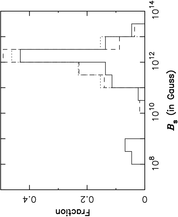
Figure 7: The surface magnetic field strength histogram of the pulsars which do not show the drifting phenomenon (solid line), those which do show the drifting phenomenon (dashed line) and those which drift coherently (dotted line). Only observations with a S/N $\geq 100$ are included.

A possible explanation for the age dependence of the drifting phenomenon is that the drift bands are more distorted for younger pulsars. One mechanism to distort the drift bands is nulling (e.g. Taylor & Huguenin 1971; van Leeuwen et al. 2002; Janssen & van Leeuwen 2004) and the fraction of time that pulsars spend in their nulling state (the nulling fraction) is known to be correlated with the pulsar age. However it has been found by Ritchings (1976) that the nulling fraction is on average higher for older pulsars, which is confirmed in later studies (e.g. Li & Wang 1995; Biggs 1992). Although the correlation with other pulsar parameters seems to be stronger, these studies prove that nulling cannot explain this correlation.

Another possible scenario is that the alignment of the magnetic dipole axis with the rotation axis has something to do with the observed trend. Observations seem to show that the angle $\alpha$ between the magnetic axis and the rotation axis is on average smaller for older pulsars (e.g. Tauris & Manchester 1998), indicating that the magnetic axis and the rotation axis becomes more aligned or anti-aligned for older pulsars. This angle is likely to be an important physical parameter in the mechanism that drives the drifting phenomenon (for instance the classical Ruderman & Sutherland 1975 model can only be applied for an anti-parallel magnetic axis). In this scenario as the pulsar gets older, the rotation axis and the magnetic axis grows more aligned, which makes the drifting mechanism more effective or regular. This trend is also consistent with the fact that pulsars with a regular drift pattern tend to have small values for $\alpha$ (Wright 2003; Rankin 1993b). However, we have found that the interpulse pulsar PSR B1702$-$19 is a coherent drifter, suggesting that coherent drifters can have a large $\alpha$ (an $\alpha$ value of $85^{\circ}$ and $90^{\circ}$ have been found by Rankin 1993b and Lyne & Manchester 1988 respectively). Also the pulse morphology seems to evolve when the pulsar ages (Rankin 1983; Beskin et al. 1984), such that core single stars are on average younger than pulsars with more complex profiles. This could make drifting subpulses more likely to be detected in older pulsars. In the non-radial pulsations model this trend can also be explained, because the appearance of narrow drifting subpulses is favored in pulsars with an aligned magnetic axis (Clemens & Rosen 2004).

An estimate for the component of the surface magnetic field of pulsars perpendicular to the rotation axis can be directly derived from the position of the pulsar in the $P$-$\dot{P}$ diagram ($B_{s}=10^{12}\sqrt{10^{15}P\dot{P}}$ Gauss). The histograms of the magnetic field strengths of the three different groups of pulsars (Fig. 7) do not show a clear trend, which is confirmed by the KS-test. It follows that the magnetic field strength distribution of the nondrifters has a chance of $\sim$20% and $\sim$50% to be statistically the same as the distributions of all the drifters (both the coherent and diffuse drifters) and the coherent drifters respectively. This means that the magnetic field strength distributions are not significantly different. If the low S/N pulsars are included, the magnetic field distributions are more likely to be the same than to be different.

It seems that the drifting phenomenon is only weakly correlated with, or even independent of magnetic field strength. This is consistent with the large fraction of pulsars that are found to show the drifting phenomenon, because the drifting phenomenon is too common to require very special physical conditions.

4.3 The drifting phenomenon and the modulation index

The drifting phenomenon is a form of subpulse modulation, so the longitude-resolved modulation index $m_{i}$ (Eq. 5) is an obvious parameter to try to correlate with the drifting phenomenon. Because the longitude-resolved modulation index can vary a lot with pulse longitude, as can be seen in the figures in appendix A, it is a somewhat arbitrary what one should call the modulation index. The longitude-resolved modulation index of many pulsars do show a minimum in the middle of the pulse profile where the total intensity is relatively high. This means that if the S/N of an observation increases, the average modulation index will also increase. This is because then the modulation index can be measured at pulse longitudes farther away from the peak intensity of the pulse profile where the longitude-resolved modulation index tends to be higher. We have therefore chosen the modulation index $m$ to be the longitude-resolved modulation index $m_{i}$ at the pulse longitude bin $i$ where $m_{i}$ has its minimum value. This definition should make the modulation index a more S/N independent number than for instance the average of the longitude-resolved modulation index. The same definition is used by Jenet & Gil (2003) to measure the modulation index.

Figure 8: The modulation index distribution of the pulsars that do not show the drifting phenomenon (solid line), that do show the drifting phenomenon (dashed line) and of the pulsars that drift coherently (dotted line). Observations with a S/N $<100$ and PSR B0531+21 (with a measured $m=5$) are not included this plot.

Modulation index histograms are shown in Fig. 8. Readily apparent is the trend that pulsars that show the drifting phenomenon more coherently have on average a lower modulation index. There seems to be no significant difference in the modulation index of the pulsars that do and do not show the drifting phenomenon. The significance of this trend is also checked with the KS-test and the modulation index distribution of the drifters is $\sim$50% as likely to be the same as the distribution of the nondrifting pulsars. The coherent drifting distribution is only 6% and 5% likely to be the same as the nondrifters and the diffuse drifting distributions respectively. These numbers are too high to state that the modulation index distribution of the coherent drifters are significantly different.

While the trend seen in Fig. 8 is not shown to be statistically significant, it is intriguing and a larger sample of pulsars is needed to determine its true significance. If the correlation is proven to be significant it would indicate that pulsars that show coherently drifting subpulses have on average a lower modulation index. Although this trend may appear counterintuitive because drifting subpulses imply subpulse modulation, it can be explained.

From the summation in Eq. 4 (and demonstrated in Fig. 3) it follows that the modulation index is independent of whether the subpulses appear randomly or organized and from Eq. 5 it follows that the modulation index is even independent of the drift band separation $P_{3}$ in the case of a coherent drifter. However, if the number of subpulses per pulse is large, the subpulses could possibly overlap causing the intensity to change less from pulse to pulse resulting in a lower modulation index (Jenet & Gil 2003). It must be noted that since sparks cannot physically overlap on the polar cap, this only works if there is significant broadening in the mapping from polar cap to the radiation beam pattern. Another parameter influencing the modulation index is the width of the subpulse intensity distribution. If the subpulses have a narrow subpulse intensity distribution, e.g. the subpulses have more equal intensities, the modulation index will also be lower. A clear example of this effect is the huge measured modulation index of PSR B0531+21 ($m=5$), caused by its giant pulses (Staelin & Reifenstein 1968).

To explain the trend that pulsars that show the drifting phenomenon coherently have on average a lower modulation index, these pulsars must either have on average more subpulses per pulse or the subpulse intensity distribution must be more narrow. In the sparking gap model it seems reasonable that the subpulses of the coherent drifters have more equal intensities. Coherent drifting could indicate that the electrodynamical conditions in the sparking gap are stable, which could be the reason why the subpulses have on average more equal intensities. Also the presence of subpulse phase steps results in a minimum in the longitude resolved modulation index (Edwards et al. 2003; Edwards & Stappers 2003b). This effect can be seen in the longitude resolved modulation index of PSR B0320+39, PSR B0809+74, PSR B1919+21 and the new drifter PSR B2255+58. Also PSR B0818$-$13 shows a minimum in its longitude resolved modulation index at the position of its subpulse phase swing. It is argued by Edwards et al. (2003) that the local reduction of the modulation index accompanied by a rapid swing in the modulation phase profile are the result of interference between two superposed drifting subpulse signals that are out of phase. It is not unlikely that interference can only occur if the drifting is coherent, which could explained the trend.

It should also be noted that the modulation index of a purely sinusoidal subpulse signal results in a modulation index of $1/\sqrt{2}$. Subpulse patterns with different waveforms or drift band shapes will generally have larger modulation indices. Many pulsars have a modulation index which is significantly lower than this value. This implies that the pulsar emission has both a subpulse signal and a non-varying component, which could indicate the presence of superposed out of phase subpulse signals.

Another explanation for this trend would be that refraction is perhaps more dominant for pulsars that do not show coherently drifting subpulses. The pulse morphology could well be influenced by refractive properties of the pulsar magnetosphere (Lyubarskii & Petrova 1998; Petrova 2000; Weltevrede et al. 2003; Fussell & Luo 2004), so it could be that for some pulsars the organized drifting subpulses are more refractively distorted than for others. For those pulsars the coherent drifting is distorted in this scenario, causing the subpulses to appear more disordered in the pulse window. Moreover it is expected that the intensities of the individual subpulses varies more because of lensing (e.g. Petrova 2000; Fussell & Luo 2004) and possible focusing of the radio emission (Weltevrede et al. 2003), causing the modulation index to be higher in those pulsars.

Figure 9: The average modulation index versus pulsar age histogram for the pulsars showing the drifting phenomenon (dashed line) and all the pulsars with a measured modulation index (solid line). The RMS is calculated as an estimate for the error (if the bin contains more than one pulsar). Pulsars with a S/N $<100$ and PSR B0531+21 ($\tau=1240$, $m=5$) are not included in this plot.

If a correlation between the drifting phenomenon and both the pulsar age and the modulation index exist, there could also be a correlation between pulsar age and modulation index. The modulation index versus pulsar age histogram is plotted in Fig. 9 and it is clear that no significant correlation is found, indicating that the modulation index is the same for pulsars with different ages. This seems to suggest that a high pulsar age and a low modulation index are two independent factors affecting the likelihood that a pulsar will exhibit coherently drifting subpulses.

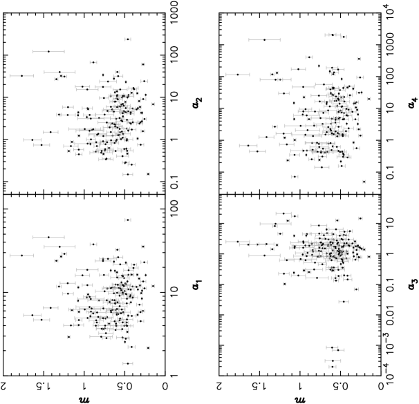
Figure 10: The modulation index for all analyzed pulsars which have a measured modulation index (except PSR B0531+21) versus the four complexity parameters as described in the text.

The modulation index of core type emission is observed by Weisberg et al. 1986 to be in general lower than that of conal type of emission. This is also a consequence of the Gil & Sendyk 2000 model. In the sparking gap model, the drifting phenomenon is associated with conal emission and therefore expected to be seen in pulsars with an on average higher modulation index. The modulation index distributions of the drifters and nondrifters are likely to be the same, so drifting phenomenon appears not to be an exclusively conal phenomenon (as suggested by Rankin 1986). If well organized coherent drifting is an exclusively conal phenomenon, it is expected that coherent drifters have an on average a higher modulation index, exactly opposite to the observed trend.

Also, if drifting is an exclusively conal phenomenon, no drifting is expected for pulsars classified as “core single stars”. Although this may be true for many cases there are some exceptions. The interpulse of PSR B1702$-$19 is classified as a core single star (Rankin 1990 and references therein) and shows a clear and narrow $P_{3}$ feature. The diffuse drifter B2255+58 is another good example of a drifter that is classified as a core single star. Most of the core single stars that show drifting are diffuse Dif^∗ drifters (PSR B0136+57, B0823+26, B1642$-$03, B1900+01, B1911$-$04, B1953+50 and B2053+36). The coherent drifter PSR B1844$-$04 has been classified as a core single or a triple profile. This means that it is questionable if the lack of of ordered subpulse modulation is a useful criterion to identify core emission (as suggested by Rankin 1986). It must be noted that the classification can be frequency dependent, so core single pulsars at low frequencies could show conal emission at higher frequencies. The many core single stars that appear to be drifting stresses the importance of being unbiased on pulsar type when studying the drifting phenomenon.

4.4 Complexity parameter

In the framework of the sparking gap model (e.g. Ruderman & Sutherland 1975; Gil & Sendyk 2000; Gil et al. 2003) the subpulses are generated (indirectly) by discharges in the polar gap (i.e. sparks). Each individual spark should emit nearly steady, unmodulated radiation, so the modulation of the pulsar emission is due to the changing positions of the subpulses in the pulse window and the number of visible sparks in different pulses. The more sparks there are visible in the pulse window, the less the intensity will change from pulse to pulse because the subpulses could overlap. The number of sparks that fits on the polar cap is quantified by the complexity parameter (Gil & Sendyk 2000) and therefore one expects an anti-correlation between the modulation index $m$ (which is a measure for how much the intensity varies from pulse to pulse) and this complexity parameter (Jenet & Gil 2003). As noted in the previous subsection, this only works if there is significant broadening in the mapping from polar cap to the radiation beam pattern.

The complexity parameter is a function of the pulse period and its derivative and its precise form depends on the model one assumes for the pulsar emission. By correlating the modulation index of a sample of pulsars with various complexity parameters as predicted by different emission models one could try to distinguish which model best fits the data (Jenet & Gil 2003). We have correlated the modulation indices in our sample of pulsars with the complexity parameter of four different emission models as derived by Jenet & Gil (2003) and Gil & Sendyk (2000):

$$\begin{array}[]{lllll}a_{1}&=&5(\dot{P}/10^{-15})^{2/7}(P/1\mathrm{s})^{-9/14},&a_{2}=&\sqrt{\dot{P}P^{-3}}\\ a_{3}&=&\sqrt{P\dot{P}},&a_{4}=&\sqrt{\dot{P}/P^{-5}}\end{array}$$ (7)

These are the complexity parameters for the sparking gap model (Gil & Sendyk 2000), continuous current outflow instabilities (Arons & Scharlemann 1979; Hibschman & Arons 2001), surface magnetohydrodynamic wave instabilities (Lou 2001) and outer magnetospheric instabilities (Jenet & Gil 2003) respectively.

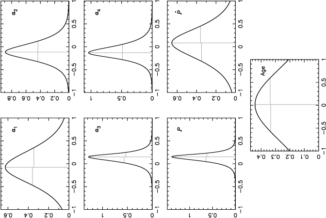
Figure 11: The probability functions $P(\rho)$ of the correlation coefficient $\rho$ for the four complexity parameters, the pulse period, the spin-down parameter and the age of the pulsar. The position of the maximum as well as the 1-$\sigma$ widths are indicated as well.

Physically, $a_{1}$ is proportional to the polar cap radius $r_{p}$ divided by the gap height $h$ as predicted in the sparking gap model and is therefore a measure for the number of sparks across the polar cap. The parameter $a_{2}$ is proportional to the acceleration parameter, which is the surface magnetic field strength $B_{\mathrm{s}}$ divided by $P^{2}$. This acceleration parameter is proportional to total current outflow from the polar cap, and roughly to the circulation time of the sparks expressed in pulse periods. The acceleration parameter is also proportional to the square root of the spin down energy loss rate. Finally $a_{3}$ and $a_{4}$ are proportional to respectively the magnetic field strength at the surface and at the light cylinder.

According to Jenet & Gil (2003) the anti-correlation between the modulation index and the complexity parameter will be masked by viewing angle issues in conal emission, so one might get better results by including only pulsars that are known to emit core emission. Because, as discussed in Sect. 4.3, it is not clear how drifting subpulses relate to the morphological classification of the pulsar, all pulsars with a measured modulation index are included in our sample. The modulation index is chosen to be the minimum in the longitude-resolved modulation index (like in Jenet & Gil 2003), which should give the best estimate for the modulation index of the core emission if present in the pulse profile.

The modulation index versus the four complexity parameters plots are shown in Fig. 10. To find out if there exist an (anti-)correlation without fitting a specific function to the data a rank-order correlation is used. This means that the rank of the values among all the other values is used rather than the values itself. This implies that the correlation coefficient is identical for the set of points ($x_{i}$, $y_{i}$) and ($F(x_{i})$, $G(y_{i})$), as long as the functions $F$ and $G$ are monotonic functions. This means that for instance, because $a_{2}$ is proportional to the square root of the spin down energy loss rate, the correlation coefficient of $a_{2}$ and the modulation index will be same as the correlation coefficient of the the spin down energy loss rate and the modulation index.

Following Jenet & Gil (2003) we have used the Spearman rank-ordered correlation coefficient $\rho$ and its significance parameter $\Delta$ (Press et al. 1992). A problem arises when one wants to include the uncertainties of the data points, because then the rank of the values is not uniquely defined anymore. As one can see in Fig. 10, the errorbars are overlapping each other, so they should be included in the analysis. The significance parameter $\Delta$ does not include the uncertainties on the data points and is therefore not directly usable to estimate the significance of $\rho$.

Parameter	correlation	coefficient ($\rho$)
$a_{1}$, $r_{\mathrm{p}}/h$	$-0.07\!$	${}^{+0.4}_{-0.4}$
$a_{2}$, $B_{\mathrm{s}}/P^{2}$	$-0.11\!$	${}^{+0.3}_{-0.3}$
$a_{3}$, $B_{\mathrm{s}}$	$0.14\!$	${}^{+0.12}_{-0.16}$
$a_{4}$, $B_{\mathrm{lc}}$	$-0.12\!$	${}^{+0.23}_{-0.20}$
$P$	$0.14\!$	${}^{+0.12}_{-0.15}$
$\dot{P}$	$0.1\!$	${}^{+0.4}_{-0.4}$
Age	$0.0\!$	${}^{+0.6}_{-0.6}$

Table 1: The correlation coefficients and their significance as derived from Fig. 11.

To include the uncertainties in the analysis we have used a Monte Carlo approach. The data points are replaced with Gaussian distributions with a width corresponding to the 1-$\sigma$ uncertainties of the measurements. In each integration step a point is randomly picked from these distributions. Instead of calculating $\rho$ and $\Delta$ directly from the data points, we calculate them for the randomly choosen points. So for each integration step we randomly select a set of points for which we get a $\rho$ and $\Delta$. The probability distribution $P(\rho)$ is calculated by averaging the Gaussian distributions centered around the calculated values of $\rho$ with a 1-$\sigma$ width $\Delta$. The calculated probablility distributions are plotted in Fig. 11. The position of the peak of the probability distribution corresponds to the most likely value of the correlation coefficient and the 1-$\sigma$ width of the peak is a measure for the significance of the correlation coefficient.

The results of this analysis are tabulated in table 1. Based on a sample of 12 pulsars, Jenet & Gil (2003) concluded that the sparking gap model ($a_{1}$) showed the highest anti-correlation and that the surface magnetohydrodynamic wave instabilities ($a_{3}$) is unlikely. Also in this enlarged sample, $a_{3}$ shows the least evidence for an anti-correlation (it is even more likely that the modulation index is positively correlated with $a_{3}$). The strongest anti-correlations are found for $a_{2}$ and $a_{4}$, which corresponds respectively to continuous current outflow instabilities and outer magnetospheric instabilities. However, none of the correlations are significantly inconsistent with an anti-correlation, and therefore none of the models can be ruled out based on these observations.

One can also see that the modulation index is uncorrelated with the age of the pulsar, which is consistent with Fig. 9. There is a hint that the modulation index is weakly correlated with the pulse period and the surface magnetic field strength $B_{\mathrm{s}}$.

4.5 Properties of drift behavior

The value of $P_{3}$ is observed to be independent of the observing frequency (Izvekova et al. 1993), but the value of $P_{2}$ could vary a little (e.g. Edwards & Stappers 2003a). Moreover observations show that measuring a value for $P_{2}$ can be far from trivial (e.g. Edwards & Stappers 2003b) and it is only a meaningful parameter if the drift bands are linear. This means that correlating $P_{3}$ with other pulsar parameters is the most direct way to find out if the drift rate depends on any physical parameters of the pulsar. The strongest correlation is expected to be found when $P_{2}$ is constant for different pulsars. Such a correlation would be a very important observational restriction on pulsar emission models.

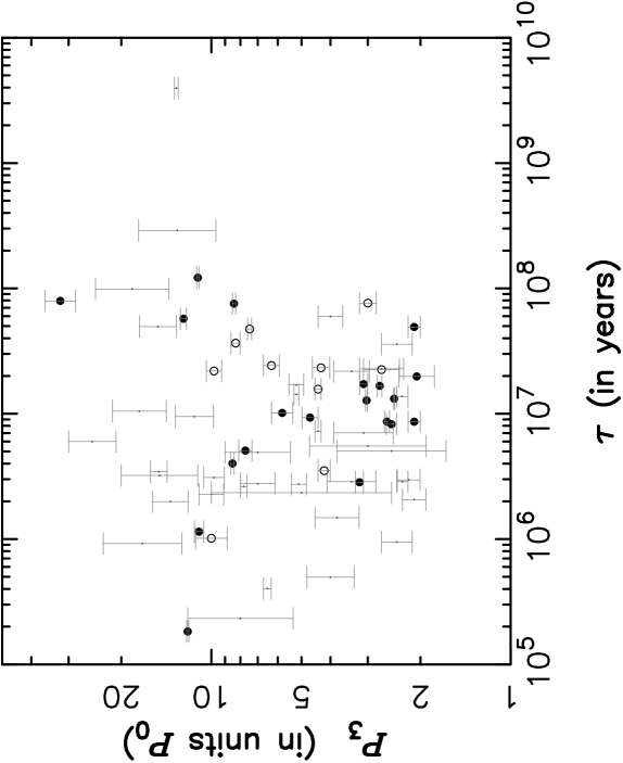
Figure 12: The measured value of the vertical drift band separation $P_{3}$ versus the pulsar age of all the pulsars showing the drifting phenomenon. The coherent drifters are the filled circles, the Dif drifters (with drift feature clearly separated from the alias borders) are the open circles and the Dif^∗ drifters are the small dots.

A significant correlation between $P_{3}$ and the pulsar age has been reported in the past (Wolszczan 1980; Ashworth 1982; Rankin 1986). As one can see in Fig. 12 there is no clear correlation present in our data, which is confirmed by $\chi^{2}$-fitting. The figure looks qualitatively the same as Fig. 4 of Rankin (1986), although she only plots “conal $P_{3}$ values”. As discussed in Sect. 4.3, it is not clear if one should make this distinction.

There is no correlation found between $P_{3}$ and the magnetic field strength, contrary to what was reported by Wolszczan (1980) and Ashworth (1982). Also there seems to be no correlation between $P_{3}$ and the pulse period (consistent with Wolszczan 1980, contrary to the tendency reported by Backer 1973). The evidence for a pulsar subpopulation located close to the $P_{3}=2P_{0}$ Nyquist limit (Wright 2003; Rankin 1986) also seems to be weak.

In a sparking gap model one would expect that the spark-associated plasma columns drift because of an $\mathbf{E}\times\mathbf{B}$ drift, which depends on both the pulse period and its derivative (e.g. Ruderman & Sutherland 1975; Gil & Sendyk 2000). The absence of any correlation between $P_{3}$ and a physical pulsar parameter is difficult to explain in this model, unless many pulsars in our sample are aliased. If a pulsar is aliased a higher $\mathbf{E}\times\mathbf{B}$ drift can result in a lower $P_{3}$ value and visa versa, making $P_{3}$ not a direct measure of the $\mathbf{E}\times\mathbf{B}$ drift. In the plot a distinction is therefore made between the coherent drifters, the diffuse Dif drifters and the Dif^∗ drifters (the latter are probably more likely to be aliased), but this separation does not reveal a significant correlation. Also if $P_{2}$ is highly variable from pulsars to pulsar, any correlation with $P_{3}$ is expected to be weaker.

There are a number of pulsars found that show evidence for drift reversals. This kind of behavior is known for PSR B2303+30 which shows drift reversals around $P_{3}=2P_{0}$ (Redman et al. 2005). This is confirmed in the 2DFS of our observation and two other other pulsars that very clearly show the same kind of behavior in its 2DFS are found: PSR B2148+63 and PSR B2310+42. Another pulsar that is known to show drift reversals is PSR B0826$-$34 (Gupta et al. 2004; Esamdin et al. 2005). This pulsar continuously changes the apparent drift direction via longitude stationary subpulse modulation. There are a few more pulsars found which possibly show the same kind of subpulse behavior: PSRs B0037+56, B1642$-$03, B1944+17, B2110+27, B2351+61. The evidence for drift reversals is less clear than for the afore mentioned $P_{3}\simeq 2P_{0}$ pulsars. If pulsars are proven to show drift reversals via longitude stationary subpulse modulation and one believes that the physical drift direction of the emission entities cannot change drift direction, it would imply that the the drifting in both drift directions is aliased.

A correlation between the drift direction and the pulsar spin-down was reported by Ritchings & Lyne (1975), such that a high spin-down is correlated with positive drifting. The same trend was also found by Ashworth (1982) and Backus (1981), although its significance was less. In our sample there is no significant correlation between the drift direction and the pulsar spin-down. Also there is no significant difference between the number of positive and negative drifters.

The value of $P_{3}$ is a much better defined parameter than $P_{2}$ if the drift bands are non linear. Although this makes it difficult to find any correlations with $P_{2}$, the fact that the drift bands can be non linear is very interesting by itself. The drift bands of for instance PSR B0809+74 (Edwards & Stappers 2003b; Prószyński & Wolszczan 1986; Wolszczan et al. 1981) and PSR B0320+39 (Edwards et al. 2003; Edwards & Stappers 2003b) show subpulse phase steps and we find that the new drifter PSR B2255+58 also shows a phase step. Although the carousel model predicts curved drift bands under certain geometries, it cannot explain sharp discontinuities of this type. A way out could be that the observed discontinuities are caused by local irregularities of the magnetic field (Wolszczan et al. 1981).

It is argued by Edwards et al. (2003) that the local reduction of the modulation index accompanied by a rapid swing in the modulation phase profile are the result of interference between two superposed drifting subpulse signals that are out of phase. In the non-radial pulsations model subpulse phase steps could be explained (Clemens & Rosen 2004), but it has trouble explaining how the modulation phase profile can be anything but piecewise linear. Visually curved drift bands are expected by applying subpulse amplitude windowing (pulse longitude dependent subpulse intensities), as pointed out by Clemens & Rosen 2004. However it is observed that the phase profile of, for example, PSR B0818$-$13 makes a swing in the middle of the pulse profile. The phase profile is not sensitive for subpulse amplitude windowing and therefore the subpulse phase swing cannot be explained by the non-radial pulsations model.

5 Summary and conclusions

Subpulse modulation is shown to be very common for radio pulsars. Of the 187 analyzed pulsars 170 are shown to exhibit subpulse modulation. The measured upper limits on the modulation index of many of the pulsars that do not have a measured modulation index were high, indicating that pulsars without any subpulse modulation are probably rare. The number of pulsars that are known to show the drifting phenomenon is significantly expanded by 42. Our sample of pulsars is not biased on pulsar type or any particular pulsar characteristics, which allows us to do meaningful statistics on the drifting phenomenon.

As the drifting phenomenon is thought to be exclusively a conal phenomenon, the modulation index of the drifters is expected to be on average higher than the modulation index of the nondrifters. The absence of such a correlation (and possible opposite trend for the coherent drifters) seems to suggest that drifting is not exclusively related to conal emission. Furthermore a number of pulsars classified as core single stars are found to show drifting, which stresses the importance to be unbiased on pulsar type when studying the drifting phenomenon.

Of the 187 analyzed pulsars 68 are shown to exhibit the drifting phenomenon (of which 30 drift coherently or have drift features clearly separated from the alias borders), which means that at least one in three pulsars show drifting. If the observations that had little chance of detecting the drifting phenomenon because of an insufficient S/N are ignored, it is shown that at least some 55% of the pulsars drift. This implies that the physical conditions required for the drifting mechanism to work cannot be very different than the required physical conditions for the emission mechanism of radio pulsars, which is consistent with the absence of a strong correlation between the drifting phenomenon and the magnetic field strength. It could well be that the drifting phenomenon is an intrinsic property of the emission mechanism, although drifting could in some cases be very difficult or even impossible to detect.

The set of modulation indices of our sample of pulsars is not shown to be inconsistent with four complexity parameters as derived for different emission models. Therefore none of the models can be ruled out based on the present observations. Other correlations are found which should be explained by emission models. The population of pulsars that show the drifting phenomenon are on average older than the population of pulsars that do not show drifting and it seems that drifting is more coherent for older pulsars.

Although significant correlations between $P_{3}$ and the pulsar age, the magnetic field strength and the pulse period have been reported previously, we find no such correlations in our enlarged sample. In a sparking gap model one would expect that the subpulses drift because of an $\mathbf{E}\times\mathbf{B}$ drift, which depends on both the pulse period and its derivative. The absence of a correlation between $P_{3}$ and any physical pulsar parameter is difficult to explain in such a model, unless many pulsars in our sample are aliased or if $P_{2}$ is highly variable from pulsar to pulsar.

No significant correlation is found between the modulation index and the pulsar age. This seems to suggest that a high pulsar age and a low modulation index are two independent factors for pulsars that affect the likelihood of them exhibiting coherently drifting subpulses. The evolutionary trend found seems to suggest that the mechanism that generates the drifting subpulses gets more and more stable as the pulsar ages, which could be because the magnetic axis and the rotation axis becomes more aligned for older pulsars.

The presence of subpulse phase steps results in a minimum in the longitude resolved modulation index. If subpulse phase steps are exclusively (or at least more likely) to occur in pulsars with coherently drifting subpulses, the modulation index of coherent drifters is expected to be on average lower. This is indeed the trend the we observe. It is argued by Edwards et al. (2003) that the local reduction of the modulation index accompanied by a rapid swing in the phase angle are the result of interference between two superposed drifting subpulse signals that are out of phase. It is not unlikely that interference can only occur if the drifting is coherent. Many pulsars are shown to have a modulation index which is significantly lower than what is expected for a purely sinusoidal subpulse signal. This implies the presence of a non-varying component in the pulsar signal, which could be caused by superposed out of phase subpulse signals.

Another possible scenario to explain the trend is that coherent drifting indicates that the electrodynamical conditions in the sparking gap are stable, which could cause the subpulses to have more equal intensities. Another explanation for this trend would be that refraction in the magnetosphere is stronger for pulsars that do not show the drifting phenomenon coherently. In that scenario the organized drifting subpulses are refracted in the magnetosphere, causing the coherent drifting to be distorted. Furthermore it is expected that refraction would cause the subpulses to appear more disordered in the pulse window and that the intensity distribution of the subpulses becomes broadened because of lensing and possible focusing of the radio emission.

[x]l—l——r—c——r—r——r—r—r@ l—r@l——l Pulsar & Class $P_{0}$ (s) $\dot{P}$ Pulses S/N  $m$      $m_{\mathrm{thresh}}$ $P_{2}$ (deg) $P_{3}$ $\;(P_{0})$ Figure
B0011+47 1.2407 $5.6\cdot 10^{-16}$ 1564 105 0.7$\pm$0.1 0.31 36
B0031$-$07 Dif 0.9430 $4.1\cdot 10^{-16}$ 1204 54 1.2$\pm$0.1 0.51 $-40\!$${}^{+2}_{-50}$ $8.3$$\pm 0.3$ 36
B0037+56 Dif^∗ 1.1182 $2.9\cdot 10^{-15}$ 2049 131 0.80$\pm$0.06 0.22 $7\!$${}^{+10}_{-2}$ $22$$\pm 3$ 36
B0052+51 Dif 2.1152 $9.5\cdot 10^{-15}$ 1112 112 0.92$\pm$0.06 0.18 $-75\!$${}^{+50}_{-50}$ $4$$\pm 2$ 36
$30\!$${}^{+70}_{-7}$ $5$$\pm 1$
B0105+65 1.2837 $1.3\cdot 10^{-14}$ 1346 71 0.43$\pm$0.04 0.33 36
J0134$-$2937 0.1370 $7.8\cdot 10^{-17}$ 4096 35 0.67 36
B0136+57 Dif^∗ 0.2725 $1.1\cdot 10^{-14}$ 3432 450 0.49$\pm$0.01 0.09 $-70\!$${}^{+15}_{-80}$ $6.5$$\pm 0.2$ 36
B0138+59 Dif^∗ 1.2229 $3.9\cdot 10^{-16}$ 2560 381 0.47$\pm$0.01 0.09 $300\!$${}^{+140}_{-110}$ $15$$\pm 4$ 36
B0144+59 0.1963 $2.6\cdot 10^{-16}$ 13534 151 1.20$\pm$0.07 0.36 36
B0148$-$06 Coh 1.4647 $4.4\cdot 10^{-16}$ 1400 135 0.59$\pm$0.04 0.22 $-12.5\!$${}^{+0.4}_{-1.9}$ $14.2$$\pm 0.2$ 36
$-45\!$${}^{+7}_{-20}$ $14.7$$\pm 0.3$
B0149$-$16 Coh 0.8327 $1.3\cdot 10^{-15}$ 1024 62 0.67$\pm$0.05 0.42 $-9\!$${}^{+12}_{-1}$ $5.8$$\pm 0.5$ 36
B0154+61 2.3517 $1.9\cdot 10^{-13}$ 769 138 1.2$\pm$0.1 0.15 36
B0301+19 Dif^∗ 1.3876 $1.3\cdot 10^{-15}$ 1263 129 0.84$\pm$0.04 0.23 $-35\!$${}^{+7}_{-55}$ $5.2$$\pm 0.3$ 36
B0320+39 Coh 3.0321 $6.4\cdot 10^{-16}$ 7169 443 0.21$\pm$0.01 0.14 $18\!$${}^{+5}_{-3}$ $8.4$$\pm 0.1$ 36
B0329+54 Dif^∗ 0.7145 $2.0\cdot 10^{-15}$ 19969 19064 0.423$\pm$0.001 0.01 $-200\!$${}^{+30}_{-150}$ $3$$\pm 2$ 36
$70\!$${}^{+13}_{-6}$ $5$$\pm 1$
B0353+52 0.1970 $4.8\cdot 10^{-16}$ 8866 117 0.63$\pm$0.06 0.28 36
B0355+54 0.1564 $4.4\cdot 10^{-15}$ 11264 1133 0.77$\pm$0.01 0.07 36
B0402+61 Lon 0.5946 $5.6\cdot 10^{-15}$ 12150 156 0.7$\pm$0.1 0.37 36
? $23$$\pm 4$
B0450+55 Dif^∗ 0.3407 $2.4\cdot 10^{-15}$ 2664 1095 0.49$\pm$0.01 0.06 $200\!$${}^{+70}_{-120}$ $20$$\pm 10$ 36
$-70\!$${}^{+8}_{-25}$ $10$$\pm 1$
B0450$-$18 0.5489 $5.8\cdot 10^{-15}$ 1537 362 0.31$\pm$0.01 0.13 36
B0458+46 0.6386 $5.6\cdot 10^{-15}$ 1440 92 0.46$\pm$0.07 0.43 36
B0523+11 Dif 0.3544 $7.4\cdot 10^{-17}$ 14849 206 0.56$\pm$0.05 0.34 $30\!$${}^{+10}_{-11}$ $3.0$$\pm 0.2$ 36
B0525+21 Dif^∗ 3.7455 $4.0\cdot 10^{-14}$ 1029 429 1.15$\pm$0.02 0.05 $-20\!$${}^{+2}_{-9}$ $3.8$$\pm 0.7$ 36
$50\!$${}^{+55}_{-10}$ $3.7$$\pm 0.4$
B0531+21 0.0331 $4.2\cdot 10^{-13}$ 178951 294 5.31$\pm$0.04 0.28 36
B0540+23 0.2460 $1.5\cdot 10^{-14}$ 3073 773 1.29$\pm$0.01 0.04 36
B0559$-$05 0.3960 $1.3\cdot 10^{-15}$ 2049 73 0.63$\pm$0.07 0.46 36
B0609+37 Coh 0.2980 $5.9\cdot 10^{-17}$ 2561 139 0.56$\pm$0.03 0.22 $-20\!$${}^{+4}_{-18}$ $32$$\pm 4$ 36
B0611+22 0.3350 $5.9\cdot 10^{-14}$ 2560 139 0.59$\pm$0.02 0.26 36
B0621$-$04 Coh 1.0391 $8.3\cdot 10^{-16}$ 1536 38 0.85$\pm$0.09 0.47 $25\!$${}^{+14}_{-16}$ $2.055$$\pm 0.001$ 36
B0626+24 0.4766 $2.0\cdot 10^{-15}$ 1025 248 0.29$\pm$0.01 0.14 36
B0628$-$28 Dif^∗ 1.2444 $7.1\cdot 10^{-15}$ 4267 1064 0.59$\pm$0.02 0.07 $30\!$${}^{+80}_{-6}$ $7$$\pm 1$ 36
B0656+14 0.3849 $5.5\cdot 10^{-14}$ 2065 292 1.24$\pm$0.03 0.10 36
B0740$-$28 0.1668 $1.7\cdot 10^{-14}$ 3585 380 0.27$\pm$0.02 0.12 36
B0751+32 Dif^∗ 1.4423 $1.1\cdot 10^{-15}$ 774 60 0.89$\pm$0.08 0.31 $-30\!$${}^{+15}_{-300}$ $5$$\pm 5$ 36
B0756$-$15 0.6823 $1.6\cdot 10^{-15}$ 1224 61 0.62$\pm$0.07 0.42 36
B0809+74 Coh 1.2922 $1.7\cdot 10^{-16}$ 13092 2635 0.496$\pm$0.001 0.04 $-16\!$${}^{+1}_{-16}$ $11.1$$\pm 0.1$ 36
B0818$-$13 Coh 1.2381 $2.1\cdot 10^{-15}$ 2251 345 0.34$\pm$0.01 0.12 $-6.5\!$${}^{+0.2}_{-0.7}$ $4.7$$\pm 0.2$ 36
B0820+02 0.8649 $1.0\cdot 10^{-16}$ 971 42 0.53$\pm$0.08 0.41 36
B0823+26 Dif^∗ 0.5307 $1.7\cdot 10^{-15}$ 1596 2635 0.967$\pm$0.001 0.01 $55\!$${}^{+40}_{-7}$ $7$$\pm 2$ 36
B0834+06 Dif^∗ 1.2738 $6.8\cdot 10^{-15}$ 1032 199 0.47$\pm$0.05 0.14 $20\!$${}^{+55}_{-9}$ $2.2$$\pm 0.2$ 36
$40\!$${}^{+140}_{-4}$ $2.1$$\pm 0.2$
B0906$-$17 0.4016 $6.7\cdot 10^{-16}$ 2115 46 0.8$\pm$0.2 0.62 36
B0919+06 Dif^∗ 0.4306 $1.4\cdot 10^{-14}$ 8255 823 0.620$\pm$0.002 0.04 $-150\!$${}^{+13}_{-75}$ $4.0$$\pm 0.8$ 36
B0950+08 0.2531 $2.3\cdot 10^{-16}$ 1311 422 1.08$\pm$0.02 0.27 36
J1022+1001 0.0165 $4.3\cdot 10^{-20}$ 211891 251 0.60$\pm$0.07 0.50 36
B1039$-$19 Dif 1.3864 $9.4\cdot 10^{-16}$ 929 160 0.51$\pm$0.08 0.18 $25\!$${}^{+9}_{-4}$ $4.3$$\pm 0.3$ 36
$9.0\!$${}^{+3.5}_{-0.1}$ $4.3$$\pm 0.1$
B1112+50 1.6564 $2.5\cdot 10^{-15}$ 1599 147 1.5$\pm$0.2 0.27 36
B1133+16 Dif^∗ 1.1879 $3.7\cdot 10^{-15}$ 1514 1156 1.4$\pm$0.1 0.04 $200\!$${}^{+55}_{-90}$ $3$$\pm 2$ 36
$130\!$${}^{+120}_{-15}$ $3$$\pm 1$
The details of all the analysed pulsars. The classification of the pulsar in the second column, where “Coh” is a coherent drifter, “Dif” and “Dif^∗” are diffuse drifters with or without drift features which are clearly separated from the alias borders and “Lon” are pulsars showing longitude stationary subpulse modulation. The next columns are the pulse period, its dimensionless time derivative, the number of pulses in the observation, the signal to noise ratio, the minimum in the longitude resolved modulation index, the minimum detectable modulation index, the horizontal and vertical driftband separation and the figure number.
Pulsar Class $P_{0}$ (s) $\dot{P}$ Pulses S/N  $m$      $m_{\mathrm{thresh}}$ $P_{2}$ (deg) $P_{3}$ $\;(P_{0})$ Figure
B1237+25 Dif^∗ 1.3824 $9.6\cdot 10^{-16}$ 1265 2121 0.480$\pm$0.002 0.04 $-20\!$${}^{+2}_{-3}$ $2.7$$\pm 0.1$ 36
$16\!$${}^{+1}_{-1}$ $2.7$$\pm 0.1$
B1254$-$10 0.6173 $3.6\cdot 10^{-16}$ 1389 14 1.58 36
B1508+55 Dif^∗ 0.7397 $5.0\cdot 10^{-15}$ 4808 568 0.52$\pm$0.01 0.09 $-160\!$${}^{+40}_{-80}$ $5$$\pm 5$ 36
J1518+4904 Dif 0.0409 $2.7\cdot 10^{-20}$ 31723 287 0.36$\pm$0.01 0.13 $55\!$${}^{+25}_{-4}$ $2.6$$\pm 0.1$ 36
B1540$-$06 Coh 0.7091 $8.8\cdot 10^{-16}$ 5121 293 0.27$\pm$0.03 0.14 $24\!$${}^{+9}_{-4}$ $3.03$$\pm 0.02$ 36
$-16\!$${}^{+12}_{-45}$ $3.02$$\pm 0.02$
B1541+09 0.7484 $4.3\cdot 10^{-16}$ 1126 93 0.47$\pm$0.07 0.41 36
B1600$-$27 0.7783 $3.0\cdot 10^{-15}$ 1077 34 0.7$\pm$0.1 0.71 36
B1604$-$00 Dif^∗ 0.4218 $3.1\cdot 10^{-16}$ 2012 1958 0.61$\pm$0.07 0.02 $55\!$${}^{+100}_{-3}$ $3.4$$\pm 0.5$ 36
$70\!$${}^{+35}_{-5}$ $3.1$$\pm 0.5$
B1612+07 1.2068 $2.4\cdot 10^{-15}$ 1926 56 0.68$\pm$0.05 0.45 36
B1642$-$03 Dif^∗ 0.3877 $1.8\cdot 10^{-15}$ 3118 656 0.337$\pm$0.002 0.06 $60\!$${}^{+9}_{-4}$ $15$$\pm 1$ 36
B1649$-$23 1.7037 $3.2\cdot 10^{-15}$ 1025 38 1.0$\pm$0.2 0.61 36
J1650$-$1654 Coh 1.7496 $3.2\cdot 10^{-15}$ 1002 55 0.7$\pm$0.1 0.49 $9\!$${}^{+7}_{-1}$ $2.59$$\pm 0.05$ 36
B1702$-$19 Coh 0.2990 $4.1\cdot 10^{-15}$ 11071 591 0.34$\pm$0.01 0.13 $-80\!$${}^{+6}_{-70}$ $11.0$$\pm 0.4$ 36
? $11.0$$\pm 0.4$
B1706$-$16 0.6531 $6.3\cdot 10^{-15}$ 1309 377 0.71$\pm$0.06 0.12 36
J1713+0747 0.0046 $8.5\cdot 10^{-21}$ 791257 181 0.60$\pm$0.04 0.40 36
B1717$-$16 1.5656 $5.8\cdot 10^{-15}$ 1120 104 0.65$\pm$0.08 0.22 36
B1717$-$29 Coh 0.6204 $7.5\cdot 10^{-16}$ 1794 17 1.0$\pm$0.2 1.24 $-9.6\!$${}^{+3}_{-0.6}$ $2.45$$\pm 0.02$ 36
B1730$-$22 0.8717 $4.3\cdot 10^{-17}$ 880 76 0.41$\pm$0.04 0.32 36
J1730$-$2304 0.0081 $2.0\cdot 10^{-20}$ 103617 76 1.52 36
B1732$-$07 0.4193 $1.2\cdot 10^{-15}$ 1826 79 0.43$\pm$0.04 0.33 36
B1736$-$29 0.3229 $7.9\cdot 10^{-15}$ 2606 26 1.0$\pm$0.2 0.89 36
B1737+13 0.8031 $1.5\cdot 10^{-15}$ 1037 30 0.9$\pm$0.2 0.73 36
B1738$-$08 Dif^∗ 2.0431 $2.3\cdot 10^{-15}$ 859 153 0.86$\pm$0.04 0.27 $60\!$${}^{+20}_{-7}$ $5.2$$\pm 0.1$ 36
$9.5\!$${}^{+4}_{-0.5}$ $4.4$$\pm 0.3$
B1744$-$24A 0.0116 $-3.4\cdot 10^{-20}$ 309244 34 2.21 36
B1745$-$12 0.3941 $1.2\cdot 10^{-15}$ 2054 75 0.49$\pm$0.08 0.49 36
B1749$-$28 0.5626 $8.1\cdot 10^{-15}$ 1285 898 0.540$\pm$0.004 0.04 36
B1753+52 Dif 2.3914 $1.6\cdot 10^{-15}$ 784 60 0.73$\pm$0.09 0.50 $100\!$${}^{+30}_{-60}$ $11$$\pm 5$ 36
$9.7\!$${}^{+3}_{-0.7}$ $6.3$$\pm 0.4$
B1754$-$24 0.2341 $1.3\cdot 10^{-14}$ 3589 113 0.58$\pm$0.06 0.27 36
B1756$-$22 0.4610 $1.1\cdot 10^{-14}$ 1561 103 0.46$\pm$0.07 0.19 36
J1757$-$2223 0.1853 $7.8\cdot 10^{-16}$ 4629 9 2.04 36
B1758$-$23 0.4158 $1.1\cdot 10^{-13}$ 2014 87 0.48 36
B1758$-$29 1.0819 $3.3\cdot 10^{-15}$ 1067 19 0.9$\pm$0.2 1.10 36
B1800$-$21 0.1336 $1.3\cdot 10^{-13}$ 6210 134 0.46$\pm$0.04 0.27 36
B1804$-$08 0.1637 $2.9\cdot 10^{-17}$ 5241 414 0.30$\pm$0.03 0.12 36
B1805$-$20 0.9184 $1.7\cdot 10^{-14}$ 1056 102 0.51$\pm$0.04 0.23 36
J1808$-$0813 0.8760 $1.2\cdot 10^{-15}$ 974 73 0.52$\pm$0.09 0.41 36
B1811+40 0.9311 $2.5\cdot 10^{-15}$ 7200 109 0.56$\pm$0.1 0.53 36
J1812$-$2102 1.2234 $2.4\cdot 10^{-14}$ 1435 63 0.65 36
B1813$-$17 0.7823 $7.3\cdot 10^{-15}$ 1096 50 0.7$\pm$0.1 0.58 36
B1815$-$14 0.2915 $2.0\cdot 10^{-15}$ 2579 175 0.27$\pm$0.03 0.18 36
B1817$-$13 0.9215 $4.5\cdot 10^{-15}$ 1031 46 0.65$\pm$0.06 0.41 36
B1818$-$04 0.5981 $6.3\cdot 10^{-15}$ 7681 353 0.40$\pm$0.04 0.16 36
B1819$-$22 Dif 1.8743 $1.4\cdot 10^{-15}$ 1096 258 0.76$\pm$0.01 0.10 $-9.1\!$${}^{+0.1}_{-1.0}$ $9.8$$\pm 0.6$ 36
B1820$-$11 0.2798 $1.4\cdot 10^{-15}$ 3021 97 0.61$\pm$0.04 0.35 36
B1821+05 0.7529 $2.3\cdot 10^{-16}$ 1080 24 0.99 36
B1821$-$11 0.4358 $3.6\cdot 10^{-15}$ 1568 59 0.37 36
B1821$-$19 0.1893 $5.2\cdot 10^{-15}$ 4105 222 0.632$\pm$0.004 0.08 36
B1822$-$09 Dif^∗ 0.7690 $5.2\cdot 10^{-14}$ 1180 409 0.672$\pm$0.005 0.24 $50\!$${}^{+110}_{-15}$ $8$$\pm 4$ 36
B1822$-$14 0.2792 $2.3\cdot 10^{-14}$ 3061 79 1.8$\pm$0.2 0.48 36
B1826$-$17 0.3071 $5.6\cdot 10^{-15}$ 2764 361 0.59$\pm$0.01 0.11 36
J1828$-$1101 0.0721 $1.5\cdot 10^{-14}$ 24167 64 0.98 36
B1829$-$08 0.6473 $6.4\cdot 10^{-14}$ 1311 132 0.56$\pm$0.09 0.22 36
B1830$-$08 0.0853 $9.2\cdot 10^{-15}$ 9412 124 1.4$\pm$0.2 0.22 36
J1830$-$1135 Dif^∗ 6.2216 $4.8\cdot 10^{-14}$ 1004 140 1.1$\pm$0.1 0.21 $25\!$${}^{+25}_{-7}$ $2.1$$\pm 0.2$ 36
continued.
Pulsar Class $P_{0}$ (s) $\dot{P}$ Pulses S/N  $m$      $m_{\mathrm{thresh}}$ $P_{2}$ (deg) $P_{3}$ $\;(P_{0})$ Figure
B1831$-$03 0.6867 $4.2\cdot 10^{-14}$ 1236 88 0.45$\pm$0.06 0.26 36
B1831$-$04 0.2901 $7.2\cdot 10^{-17}$ 11255 114 0.41$\pm$0.05 0.36 36
B1832$-$06 0.3058 $4.0\cdot 10^{-14}$ 4557 33 0.98 36
B1834$-$04 0.3542 $1.7\cdot 10^{-15}$ 4114 73 0.57$\pm$0.05 0.41 36
B1834$-$10 0.5627 $1.2\cdot 10^{-14}$ 1286 151 0.32$\pm$0.01 0.12 36
J1835$-$1106 0.1659 $2.1\cdot 10^{-14}$ 5125 108 0.89$\pm$0.04 0.42 36
B1839+09 0.3813 $1.1\cdot 10^{-15}$ 2056 79 0.48$\pm$0.06 0.41 36
B1839+56 1.6529 $1.5\cdot 10^{-15}$ 1031 53 1.07$\pm$0.06 0.44 36
B1839$-$04 Coh 1.8399 $5.1\cdot 10^{-16}$ 1025 179 0.49$\pm$0.04 0.15 $-35\!$${}^{+5}_{-15}$ $12.4$$\pm 0.3$ 36
$120\!$${}^{+20}_{-20}$ $12.4$$\pm 0.3$
J1839$-$0643 0.4495 $3.6\cdot 10^{-15}$ 3590 50 0.51$\pm$0.08 0.47 36
B1841$-$04 Coh 0.9910 $3.9\cdot 10^{-15}$ 1551 69 0.62$\pm$0.09 0.44 $-13\!$${}^{+11}_{-5}$ $8.5$$\pm 0.1$ 36
B1841$-$05 0.2557 $9.7\cdot 10^{-15}$ 3077 115 0.26$\pm$0.04 0.26 36
B1842+14 0.3755 $1.9\cdot 10^{-15}$ 3073 77 0.67$\pm$0.06 0.46 36
B1842$-$04 0.4868 $1.1\cdot 10^{-14}$ 1556 68 0.53$\pm$0.07 0.45 36
B1844$-$04 Coh 0.5978 $5.2\cdot 10^{-14}$ 1240 115 0.38$\pm$0.03 0.26 $80\!$${}^{+70}_{-45}$ $12$$\pm 1$ 36
B1845$-$01 Dif^∗ 0.6594 $5.3\cdot 10^{-15}$ 1031 213 0.28$\pm$0.01 0.11 $90\!$${}^{+170}_{-35}$ $14$$\pm 2$ 36
J1845$-$0743 0.1047 $3.7\cdot 10^{-16}$ 8193 115 1.02$\pm$0.09 0.26 36
B1846$-$06 Lon 1.4513 $4.6\cdot 10^{-14}$ 1208 128 1.31$\pm$0.03 0.24 ? $3$$\pm 1$ 36
B1848+13 0.3456 $1.5\cdot 10^{-15}$ 1544 42 0.55$\pm$0.09 0.55 36
B1849+00 2.1802 $9.7\cdot 10^{-14}$ 1030 94 0.25$\pm$0.02 0.17 36
J1850+0026 1.0818 $3.6\cdot 10^{-16}$ 1029 41 0.61$\pm$0.08 0.38 36
J1852+0305 1.3261 $1.0\cdot 10^{-16}$ 1323 10 2.21 36
J1852$-$2610 0.3363 $8.8\cdot 10^{-17}$ 2526 42 0.50 36
B1855+02 0.4158 $4.0\cdot 10^{-14}$ 2051 77 0.7$\pm$0.1 0.49 36
B1855+09 0.0054 $1.8\cdot 10^{-20}$ 158193 175 0.6$\pm$0.1 0.46 36
B1857$-$26 Dif 0.6122 $2.0\cdot 10^{-16}$ 1339 360 0.47$\pm$0.02 0.20 $80\!$${}^{+80}_{-9}$ $7.5$$\pm 0.2$ 36
$180\!$${}^{+20}_{-45}$ $7.3$$\pm 0.2$
B1859+03 0.6555 $7.5\cdot 10^{-15}$ 1552 182 0.35$\pm$0.05 0.12 36
B1859+07 0.6440 $2.3\cdot 10^{-15}$ 1030 46 0.47$\pm$0.08 0.52 36
B1900+01 Dif^∗ 0.7293 $4.0\cdot 10^{-15}$ 1171 327 0.56$\pm$0.05 0.09 $30\!$${}^{+30}_{-3}$ $3.4$$\pm 0.7$ 36
B1900+05 0.7466 $1.3\cdot 10^{-14}$ 1025 54 0.49$\pm$0.06 0.40 36
J1901$-$0906 Coh 1.7819 $1.6\cdot 10^{-15}$ 785 147 0.47$\pm$0.08 0.13 $-11\!$${}^{+1}_{-8}$ $6.9$$\pm 0.3$ 36
$-5.6\!$${}^{+0.1}_{-0.7}$ $3.1$$\pm 0.1$
B1903+07 0.6480 $4.9\cdot 10^{-15}$ 2246 32 0.72 36
B1905+39 1.2358 $5.4\cdot 10^{-16}$ 1032 50 0.78$\pm$0.07 0.57 36
B1907+00 1.0169 $5.5\cdot 10^{-15}$ 1030 40 0.63$\pm$0.06 0.44 36
B1907+10 0.2836 $2.6\cdot 10^{-15}$ 3023 95 0.51$\pm$0.07 0.44 36
B1910+20 2.2330 $1.0\cdot 10^{-14}$ 1025 43 0.67$\pm$0.07 0.39 36
B1911+13 0.5215 $8.0\cdot 10^{-16}$ 2055 56 0.32$\pm$0.04 0.26 36
B1911$-$04 Dif^∗ 0.8259 $4.1\cdot 10^{-15}$ 2082 616 0.287$\pm$0.004 0.08 $70\!$${}^{+40}_{-30}$ $15$$\pm 5$ 36
B1914+09 0.2703 $2.5\cdot 10^{-15}$ 6145 97 0.59$\pm$0.08 0.52 36
B1914+13 0.2818 $3.6\cdot 10^{-15}$ 4096 185 0.41$\pm$0.02 0.19 36
B1915+13 0.1946 $7.2\cdot 10^{-15}$ 1541 41 0.46 36
B1916+14 1.1810 $2.1\cdot 10^{-13}$ 1226 23 0.79 36
B1917+00 Dif^∗ 1.2723 $7.7\cdot 10^{-15}$ 4106 135 0.69$\pm$0.08 0.27 $70\!$${}^{+7}_{-25}$ $7.8$$\pm 0.2$ 36
B1918+19 0.8210 $9.0\cdot 10^{-16}$ 1550 60 0.58$\pm$0.07 0.48 36
B1919+21 Dif 1.3373 $1.3\cdot 10^{-15}$ 1033 207 0.30$\pm$0.04 0.18 $-3.4\!$${}^{+0.3}_{-0.2}$ $4.4$$\pm 0.1$ 36
$-11\!$${}^{+1}_{-1}$ $4.4$$\pm 0.1$
B1920+21 1.0779 $8.2\cdot 10^{-15}$ 1025 74 0.40$\pm$0.06 0.30 36
B1924+16 0.5798 $1.8\cdot 10^{-14}$ 2514 87 0.76$\pm$0.06 0.44 36
B1929+10 Dif^∗ 0.2265 $1.2\cdot 10^{-15}$ 1324 681 0.466$\pm$0.002 0.04 $90\!$${}^{+140}_{-8}$ $9.8$$\pm 0.8$ 36
$-160\!$${}^{+10}_{-100}$ $4.4$$\pm 0.1$
B1933+16 Dif^∗ 0.3587 $6.0\cdot 10^{-15}$ 2613 2081 0.240$\pm$0.001 0.02 $300\!$${}^{+130}_{-50}$ $2.4$$\pm 0.3$ 36
B1935+25 0.2010 $6.4\cdot 10^{-16}$ 7173 66 0.58$\pm$0.06 0.47 36
B1937+21 0.0016 $1.1\cdot 10^{-19}$ 600160 339 0.19 36
B1937$-$26 Lon 0.4029 $9.6\cdot 10^{-16}$ 2129 91 0.93$\pm$0.08 0.31 ? $2.5$$\pm 0.5$ 36
B1943$-$29 0.9594 $1.5\cdot 10^{-15}$ 1319 43 0.8$\pm$0.1 0.56 36
B1944+17 Dif^∗ 0.4406 $2.4\cdot 10^{-17}$ 2056 278 1.19$\pm$0.02 0.17 $-11.7\!$${}^{+0.3}_{-0.3}$ $13$$\pm 5$ 36
B1946+35 Lon 0.7173 $7.1\cdot 10^{-15}$ 1161 176 0.43$\pm$0.01 0.12 ? $33$$\pm 2$ 36
continued.
Pulsar Class $P_{0}$ (s) $\dot{P}$ Pulses S/N  $m$      $m_{\mathrm{thresh}}$ $P_{2}$ (deg) $P_{3}$ $\;(P_{0})$ Figure
B1952+29 Dif^∗ 0.4267 $1.7\cdot 10^{-18}$ 1536 312 0.46$\pm$0.06 0.07 $-190\!$${}^{+15}_{-170}$ $13.1$$\pm 0.2$ 36
$-40\!$${}^{+6}_{-30}$ $12.5$$\pm 0.4$
B1953+50 Dif^∗ 0.5189 $1.4\cdot 10^{-15}$ 1635 464 0.9$\pm$0.2 0.08 $5.3\!$${}^{+16}_{-0.2}$ $25$$\pm 7$ 36
B2000+32 0.6968 $1.1\cdot 10^{-13}$ 2060 90 0.8$\pm$0.1 0.41 36
B2000+40 Coh 0.9051 $1.7\cdot 10^{-15}$ 768 109 0.53$\pm$0.04 0.28 $-7.3\!$${}^{+0.8}_{-0.6}$ $2.5$$\pm 0.1$ 36
$-17\!$${}^{+3}_{-8}$ $2.5$$\pm 0.1$
B2002+31 2.1113 $7.5\cdot 10^{-14}$ 1115 214 0.54$\pm$0.02 0.12 36
B2003$-$08 0.5809 $4.6\cdot 10^{-17}$ 1285 37 0.8$\pm$0.2 0.74 36
B2011+38 Lon 0.2302 $8.9\cdot 10^{-15}$ 3722 271 1.34$\pm$0.02 0.21 ? $30$$\pm 15$ 36
B2016+28 Dif^∗ 0.5580 $1.5\cdot 10^{-16}$ 25899 511 0.61$\pm$0.01 0.15 $-70\!$${}^{+15}_{-25}$ $20$$\pm 2$ 36
$-12\!$${}^{+1}_{-8}$ $4.0$$\pm 0.4$
B2020+28 Dif^∗ 0.3434 $1.9\cdot 10^{-15}$ 3759 1438 0.15$\pm$0.02 0.04 $-55\!$${}^{+5}_{-15}$ $2.5$$\pm 0.2$ 36
$25\!$${}^{+15}_{-2}$ $2.3$$\pm 0.1$
B2021+51 Dif^∗ 0.5292 $3.1\cdot 10^{-15}$ 20326 1180 0.50$\pm$0.03 0.08 $10\!$${}^{+15}_{-1}$ $5.1$$\pm 0.3$ 36
B2022+50 0.3726 $2.5\cdot 10^{-15}$ 2278 96 0.52$\pm$0.04 0.31 36
B2043$-$04 Coh 1.5469 $1.5\cdot 10^{-15}$ 1025 122 0.69$\pm$0.02 0.23 $4.5\!$${}^{+5}_{-0.3}$ $2.74$$\pm 0.05$ 36
B2044+15 Dif^∗ 1.1383 $1.8\cdot 10^{-16}$ 768 51 0.72$\pm$0.06 0.40 $-7.1\!$${}^{+0.5}_{-1.4}$ $18$$\pm 6$ 36
B2045$-$16 Coh 1.9616 $1.1\cdot 10^{-14}$ 384 44 0.8$\pm$0.1 0.55 $17\!$${}^{+18}_{-2}$ $3.2$$\pm 0.1$ 36
B2053+36 Dif^∗ 0.2215 $3.7\cdot 10^{-16}$ 3594 173 0.59$\pm$0.02 0.22 $100\!$${}^{+340}_{-75}$ $11$$\pm 2$ 36
B2106+44 Lon 0.4149 $8.6\cdot 10^{-17}$ 2067 292 0.52$\pm$0.04 0.19 ? $19$$\pm 7$ 36
B2110+27 Dif^∗ 1.2029 $2.6\cdot 10^{-15}$ 1032 370 1.06$\pm$0.02 0.09 $140\!$${}^{+18}_{-15}$ $4.4$$\pm 0.1$ 36
B2111+46 Dif 1.0147 $7.1\cdot 10^{-16}$ 3083 258 0.62$\pm$0.05 0.17 $-180\!$${}^{+20}_{-50}$ $2.7$$\pm 0.4$ 36
J2145$-$0750 0.0161 $3.0\cdot 10^{-20}$ 224536 190 0.53$\pm$0.07 0.16 36
B2148+52 0.3322 $1.0\cdot 10^{-14}$ 2055 89 0.39$\pm$0.06 0.34 36
B2148+63 Dif^∗ 0.3801 $1.7\cdot 10^{-16}$ 2256 143 0.89$\pm$0.02 0.26 $-35\!$${}^{+7}_{-15}$ $2.4$$\pm 0.3$ 36
B2154+40 Dif^∗ 1.5253 $3.4\cdot 10^{-15}$ 1148 475 0.60$\pm$0.01 0.11 $110\!$${}^{+80}_{-10}$ $3.1$$\pm 0.8$ 36
B2217+47 0.5385 $2.8\cdot 10^{-15}$ 1592 191 0.52$\pm$0.03 0.18 36
B2224+65 0.6825 $9.7\cdot 10^{-15}$ 2548 56 0.96$\pm$0.07 0.42 36
B2255+58 Dif 0.3682 $5.8\cdot 10^{-15}$ 2305 506 0.52$\pm$0.01 0.12 $11\!$${}^{+11}_{-1}$ $10$$\pm 1$ 36
B2303+30 Coh 1.5759 $2.9\cdot 10^{-15}$ 1109 96 0.72$\pm$0.08 0.26 $15.0\!$${}^{+3}_{-0.3}$ $2.1$$\pm 0.1$ 36
B2306+55 0.4751 $2.0\cdot 10^{-16}$ 3596 45 0.8$\pm$0.1 0.70 36
B2310+42 Coh 0.3494 $1.1\cdot 10^{-16}$ 5006 2073 0.46$\pm$0.01 0.11 $60\!$${}^{+20}_{-10}$ $2.1$$\pm 0.1$ 36
$6.0\!$${}^{+0.3}_{-0.3}$ $2.1$$\pm 0.1$
B2315+21 1.4447 $1.0\cdot 10^{-15}$ 1024 44 0.7$\pm$0.1 0.58 36
B2319+60 Coh 2.2565 $7.0\cdot 10^{-15}$ 1041 1652 0.923$\pm$0.004 0.03 $70\!$${}^{+60}_{-10}$ $7.7$$\pm 0.4$ 36
$12\!$${}^{+4}_{-1}$ $7.7$$\pm 0.1$
B2323+63 1.4363 $2.8\cdot 10^{-15}$ 1036 29 1.6$\pm$0.1 0.67 36
B2324+60 Dif^∗ 0.2337 $3.5\cdot 10^{-16}$ 3633 289 0.95$\pm$0.01 0.16 $160\!$${}^{+40}_{-30}$ $17$$\pm 4$ 36
B2327$-$20 1.6436 $4.6\cdot 10^{-15}$ 1024 125 0.55$\pm$0.04 0.15 36
B2334+61 0.4953 $1.9\cdot 10^{-13}$ 3085 19 1.3$\pm$0.2 1.07 36
J2346$-$0609 Dif^∗ 1.1815 $1.4\cdot 10^{-15}$ 770 79 0.77$\pm$0.04 0.22 $-90\!$${}^{+25}_{-120}$ $2.3$$\pm 0.1$ 36
B2351+61 Dif^∗ 0.9448 $1.6\cdot 10^{-14}$ 7655 661 1.07$\pm$0.01 0.07 $60\!$${}^{+25}_{-8}$ $17$$\pm 6$ 36
continued.

Astro-ph version is missing 187 figures due to file size restrictions. Please download appendices from http://www.science.uva.nl/$\sim$wltvrede/21cm.pdf.

Appendix A Figures

Figure 13:

Figure 14:

Figure 15:

Figure 16:

Figure 17:

Figure 18:

Figure 19:

Figure 20:

Figure 21:

Figure 22:

Figure 23:

Figure 24:

Figure 25:

Figure 26:

Figure 27:

Figure 28:

Figure 29:

Figure 30:

Figure 31:

Figure 32:

Figure 33:

Figure 34:

Figure 35:

Figure 36:

Appendix B Figures ordered by appearance in text