Galactic structure from the Calar Alto Deep Imaging Survey (CADIS)

We used 1627 faint ($15.5\leq R\leq 23$) stars in five fields of the Calar Alto Deep Imaging Survey (CADIS) to estimate the structure parameters of the Galaxy. The results were derived by applying two complementary methods: first by fitting the density distribution function to the measured density of stars perpendicular to the Galactic plane, and second by modelling the observed colors and apparent magnitudes of the stars in the field, using Monte Carlo simulations. The best-fitting model of the Galaxy is then determined by minimising the C-statistic, a modified $\chi^{2}$. Our model includes a double exponential for the stellar disk with scaleheights $h_{1}$ and $h_{2}$ and a power law halo with exponent $\alpha$. $24\,480$ different parameter combinations have been simulated. Both methods yield consistent results: the best fitting parameter combination is $\alpha=3.0$ (or $\alpha=2.5$, if we allow for a flattening of the halo with an axial ratio of $(c/a)=0.6$), $h_{1}=300$ pc, $h_{2}=900$ pc, and the contribution of thick disk stars to the disk stars in the solar neighbourhood is found to be between 4 and 10 %.

1 Introduction

The stellar structure of our own Galaxy has been studied intensively for almost 400 years now, and although, or perhaps exactly because of the fact that the subject to be analysed is our own neighbourhood and surrounds us, there are still a large number of unknowns and the exact structure parameters are still a topic of debate.

In the standard model (Bahcall & Soneira 1980a, b) the Galaxy is of Hubble type $Sbc$, consisting of an exponential disk, a central bulge, and a spherical halo. The vertical structure of the disk follows an exponential law ($\rho\propto e^{-z/h_{z}}$) with scaleheight $h_{z}=325$ pc. However, as Gilmore & Reid (1983) showed, the data can be fitted much better by a superposition of two exponentials with scaleheights $h_{1}$ of $90$ to $325$ pc and $h_{2}\approx 1300$ pc (Gilmore 1984). It is not clear whether this deviation from the single exponential is due to a distinct population of stars, although this is suggested by the different kinematics and lower metallicities (Freeman 1992), it is referred to as ”thick disk” in the literature.

In the last two decades highly efficient, large area surveys have been carried out, and large quantities of high-quality imaging data have been produced. The mere existance of a thick disk component is fairly established today, however, the size of its scaleheights are still under discussion (Norris 1999; Siegel et al. 2002), as several authors claim to have found a considerably smaller value for the scaleheight of the thick disk than the canonical one of $h_{2}\sim 1.3$ kpc: Robin et al. (2000) found 750 pc, and Chen et al. (2001) found the scaleheight to be between 580 and 750 pc.

In general there are two different approaches to deduce Galactic Structure: the Baconian, and the Cartesian ansatz, as Gilmore & Wyse (1987) call it.

The Baconian ansatz tries to manage with a minimum of assumptions: by a pure measurement of the stellar distribution function by means of starcounts. Distances are estimated for each star and then their number density in dependence of distance from the Galactic plane is calculated (Gilmore & Reid 1983; Reid et al. 1996, 1997; Gould et al. 1998). The parameters can then be determined by fitting distribution functions to the data. In a first paper on CADIS deep star counts (Phleps et al. 2000, Paper I in the following) we presented first results based on $\approx 300$ faint stars ($15.5\leq R\leq 23$) in two CADIS fields covering an area of $\sim 1/15\leavevmode\nobreak\ \squareforqed\degr$ in total. From these data we deduced the density distribution of the stars up to a distance of about 20 kpc above the Galactic plane, using the Baconian ansatz. We found $h_{1}=280$ pc, and unambigously the contribution of the thick disk with $h_{2}$ on the order of $1300$ pc.

On the other hand, as the main structural features of the Milky Way have been identified, it has been possible to design synthetic models of the Galactic stellar populations (Bahcall & Soneira 1981; Gilmore 1984; Robin & Creze 1986; Reid & Majewski 1993; Mendez & van Altena 1998; Chen et al. 1999, 2001), assuming the forms of the density distribution function for the different components of the Galaxy. This method is what Gilmore & Wyse (1987) call the Cartesian ansatz.

The exact structure parameters can then be deduced by comparing model and star count data.

In this paper we use both approaches using the stellar component of the CADIS data. Deep ($R<23$) multi color data is now available for 1627 faint stars in five fields at high Galactic latitude and different Galactic longitudes.

In Section 2 the Calar Alto Deep Imaging Survey is briefly described. In Section 4 the results we deduced by applying the ”classic”, Baconian method are shown, whereas in Section 5 we show the results given by the modelling approach. A summary and discussion is given in Section 6.

2 The Calar Alto Deep Imaging Survey

The Calar Alto Deep Imaging Survey was established in 1996 as the extragalactic key project of the Max-Planck Institut für Astronomie. It combines a very deep emission line survey carried out with an imaging Fabry-Perot interferometer with a deep multicolour survey using three broad-band optical to NIR filters and up to thirteen medium-band filters. The combination of different observing strategies facilitates not only the detection of emission line objects but also the derivation of photometric spectra of all objects in the fields without performing time consuming slit spectroscopy.

The seven CADIS fields measure $\approx 1/30\leavevmode\nobreak\ \squareforqed\degr$ each ($11^{\prime\prime}\times 11^{\prime\prime}$) and are located at high Galactic latitudes to avoid dust absorption and reddening. In all fields the total flux on the IRAS 100 $\mu$m maps is less than 2 MJy/sr which corresponds to $E_{B-V}<0.07$. Therefore we do not have to apply any colour corrections. As a second selection criterium the fields should not contain any star brighter than $\approx 16^{mag}$ in the CADIS $R$ band. In fact the brightest star in the five fields under consideration has an $R$ magnitude of $15.42^{mag}$.

All observations were performed on Calar Alto, Spain. In the optical wavelength region the focal reducers CAFOS (Calar Alto Faint Object Spectrograph) at the 2.2 m telescope and MOSCA (Multi Object Spectrograph for Calar Alto) at the 3.5 m telescope were used. The NIR observations have been carried out using the Omega Prime camera at the 3.5m telescope.

In each filter, a set of 5 to 15 individual exposures was taken. The images of one set were then bias subtracted, flatfielded and corrected for cosmic ray hits, and then coadded to one deep sumframe. This basic data reduction steps were done with the MIDAS software package in combination with the data reduction and photometry package MPIAPHOT (developed by H.-J. Röser and K. Meisenheimer).

2.1 Object detection and classification

Object search is done on the sumframe of each filter using the source extractor software SExtractor (Bertin & Arnouts 1996). The filter-specific object lists are then merged into a master list containing all objects exceeding a minimum $S/N$ ratio in any of the bands. Photometry is done using the program Evaluate, which has been developed by Meisenheimer and Röser (see Meisenheimer & Röser 1986, and Röser & Meisenheimer 1991). Variations in seeing between individual exposures are taken into account, in order to get accurate colours. Because the photometry is performed on individual frames rather than sumframes, realistic estimates of the photometric errors can be derived straightforwardly.

The measured counts are translated into physical fluxes outside the terrestrial atmosphere by using a set of ”tertiary” spectrophotometric standard stars which were established in the CADIS fields, and which are calibrated with secondary standard stars (Oke 1990; Walsh 1995) in photometric nights.

From the physical fluxes, magnitudes and colour indices (an object’s brightness ratio in any two filters, usually given in units of magnitudes) can be calculated. The CADIS magnitude system is described in detail in Wolf et al. (2001b) and Fried et al. (2001).

The CADIS color is defined by:

$$(b-r)=2.5\log\frac{F_{R}^{\gamma}}{F_{B}^{\gamma}}\leavevmode\nobreak\ .$$ (1)

Here $F^{\gamma}_{k}$ is the flux outside the atmosphere in units of Photons ${\rm m}^{-2}\leavevmode\nobreak\ {\rm s}^{-1}\leavevmode\nobreak\ {\rm nm}^{-1}$ in the CADIS filter $k$.

$b-r$ can be calibrated to the Johnson-Cousins system (the CADIS $R_{C}$ is very close to the Cousins $R$) by using Vega as a zero point:

$$(B-R)_{C} = (b-r)+2.5\log\frac{F^{\gamma}_{{\rm Vega}}(\lambda=440{\rm nm})}{F^{\gamma}_{{\rm Vega}}(\lambda=648{\rm nm})}$$ (2)

$$= (b-r)+0.725\leavevmode\nobreak\ .$$

With a typical seeing of $1\aas@@fstack{\prime\prime}5$ a morphological star-galaxy separation becomes unreliable at $R\ga 21$ where already many galaxies appear compact. Quasars have point-like appearance, and thus can not be distinguished from stars by morphology. Therefore a classification scheme was developed, which is based solely on template spectral energy distributions ($SED$s) (Wolf et al. 2001b, a). The classification algorithm basically compares the observed colours of each object with a colour library of known objects. This colour library is assembled from observed spectra by synthetic photometry performed on an accurate representation of the instrumental characteristics used by CADIS. As input for the stellar library we used the catalogue by Pickles (1998).

Using the minimum variance estimator (for details see Wolf et al. 2001b), each object is assigned a type (star – QSO – galaxy), a redshift (if it is not classified as star), and an $SED$.

Note that we do not apply any morphological star/galaxy separation or use other criteria. The classification is purely spectrophotometric.

Five CADIS fields have been fully analysed so far (for coordinates see Table 1). We identified 1627 stars with $R\leq 23$. The number of stars per field is given in Table 1.

Table 1: The Galactic coordinates of the five fields investigated so far, and the number of stars per field, $R\leq 23$.

CADIS field	$l$	$b$	$N_{stars}$
1 h	$150^{\circ}$	$-59^{\circ}$	$200$
9 h	$175^{\circ}$	$45^{\circ}$	$300$
13 h	$335^{\circ}$	$60^{\circ}$	$517$
16 h	$85^{\circ}$	$45^{\circ}$	$390$
23 h	$90^{\circ}$	$-43^{\circ}$	$220$

3 The stellar density distribution

Since none of our fields points towards the Galactic center and all of them are located at high Galactic latitudes, neither a bulge component nor spiral arms are needed to describe the observations. Our model of the density distribution of the stars includes only a disk and a halo.

3.1 The distribution of stars in the Galactic disk

The vertical density distribution of stars in the disk is described by a sum of two exponentials (the “thin” and a “thick” disk component):

$$\rho(z)=\left[n_{1}\exp\left(-\frac{z}{h_{1}}\right)+n_{2}\exp\left(-\frac{z}{h_{2}}\right)\right]\leavevmode\nobreak\ ,$$ (3)

where $z$ is the vertical distance from the Galactic plane, $n_{1}$ and $n_{2}$ are the normalisations at $z=0$, and $h_{1}$ and $h_{2}$ are the scaleheights of thin and thick disk, respectively.

The radial change of the density can be taken into account by assuming an exponential decrease with scalelength $h_{r}$. The value of $h_{r}$ is still poorly determined, measurements range from values as small as $h_{r}=2$ kpc (Robin et al. 1992; Ruphy et al. 1996; Ojha et al. 1996; Bienaymé 1999) to $h_{r}=3.5$ kpc (Bahcall & Soneira 1980b, 1981; Wainscoat et al. 1992).

For each field with Galactic longitude $l$ and latitude $b$, respectively, we can describe the distribution of the stars in the disk by

$$\rho_{d}(r,l,b)=\left[n_{1}\exp\left(-\frac{r\sin b}{h_{1}}\right)+n_{2}\exp\left(-\frac{r\sin b}{h_{2}}\right)\right]$$ (4)

$$\cdot\exp\left[-\frac{\sqrt{r^{2}-2R_{\odot}\frac{r\sin b}{\tan b}\cos l+r^{2}\sin^{2}b}+R_{\odot}}{h_{r}}\right]\leavevmode\nobreak\ .$$

The distance of the sun from the Galacic center is assumed to be $R_{\odot}=8$ kpc.

3.2 The distribution of stars in the Galactic halo

The space density corresponding to the $r^{1/4}$ law in projection has no simple analytic form (Young 1976). There are different possibilities to find an approximation, the simplest of which is a power law (Fuchs & Jahreiß 1998) of the form

$$\rho=\rho_{\odot}\cdot\left[\frac{r_{c}^{2}+R_{\odot}^{2}}{r_{c}^{2}+r^{2}}\right]^{\alpha/2}\leavevmode\nobreak\ ,$$ (5)

with an arbitrarily chosen core radius of $r_{c}=1$ kpc, and

$$r=R_{\odot}^{2}+\frac{z^{2}}{\sin^{2}b}-2R_{\odot}\frac{z}{\tan b}\cos l+\frac{z^{2}}{(c/a)^{2}}\leavevmode\nobreak\ .$$ (6)

Several authors found that the stellar halo is significantly flattened, with an axial ratio of $(c/a)$ around $0.6$ (Robin et al. 2000; Lemon et al. 2004.

4 Star Counts – a direct measurement

Now, as we have more than twice the number of fields available than in our first analysis, and due to the increased number of filters used for the classification of the objects, the statistics has increased considerably, from $\sim 300$ stars in Paper I to $\sim 1630$ now.

Figure (1) shows the distribution of measured colors of the selected stars in the field. As in our first analysis, we use this bimodal distribution of colors, which comes from the interaction between luminosity function, density distribution and apparent magnitude limits ($15.5\leq R\leq 23$), to discriminate between disk and halo stars. The nearby disk stars are intrinsically faint and therefore red, whereas the halo stars have to be bright enough to be seen at large distances, and are therefore blue. According to the different directions of the fields the cut is located at slightly different colors, as indicated in Figure 1. Unfortunately it is not possible to dicriminate between thin and thick disk stars in the same way, so in the calculation of absolute magnitudes and thus distances we have to treat them in the same way.

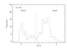
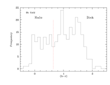
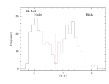
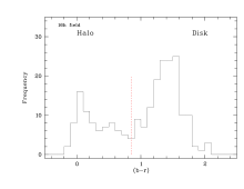
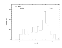
Figure 1: The distribution of observed $(b-r)_{C}$ colors in the fields. The dotted line shows the color cut between halo and disk. Note that the ordinate has not the same scale in all cases, whereas the dotted line extends to 20 in each plot. The maxima are not located at the same colors, but depend on the direction of the field.

We repeated the calculation of the photometric parallaxes of the stars exactly as described in Paper I. Absolute magnitudes are inferred from a mean main sequence relation in a color-magnitude diagram (Lang 1992). The main sequence converted into a $M_{R}$ vs $(b-r)$ relation (see Paper I) can be approximated by a fourth order polynomial in the range $-2\leq(b-r)\leq 1.8$:

$$M_{R} = c_{0}+c_{1}\leavevmode\nobreak\ (b-r)+c_{2}\leavevmode\nobreak\ (b-r)^{2}$$ (7)

$$+ c_{3}\leavevmode\nobreak\ (b-r)^{3}+c_{4}\leavevmode\nobreak\ (b-r)^{4},$$

the parameters of which are:

$c_{0}=4.01236$       $c_{1}=4.12575$       $c_{2}=-1.89076$       $c_{3}=0.762053$       $c_{4}=0.341384$ .

This main sequence approximation is valid for all stars in our sample since we can be sure that it is free from contamination of any non-main sequence stars, as the faint magnitude intervall we observe ($16\leq R\leq 23$) does not allow the detection of a giant star.

The mean main sequence relation is valid strictly only for stars with solar metallicities, whereas our sample may contain stars spread over a wide range of different metalicities. The influence of the varying metalicities on the main sequence color-magnitude relation is taken into account as described in Paper I: Halo stars are supposed to be metal poor, and are known to be fainter than disk stars with the same colors, so the relation is shifted towards fainter magnitudes by $\Delta M_{R}=0.75$. This value is the mean deviation from the mean main sequence defined by the CNS4 stars (Jahreiß & Wielen 1997) of a subsample of 10 halo stars for which absolute $R$ magnitudes were available (Jahreiß, priv. com).

The spread in a two color diagram $(b-r)$ versus $(r-i)$ (that is the CADIS color between $R_{C}$ and $I_{815}$, analog to Eq. 1) becomes significant at $(b-r)\approx 1.0$, see Fig. 2. The maximal photometric error for the very faint stars is $0.15^{mag}$. Here metallicity effects will distort the relation between the measured $(b-r)$ colors and the spectral type (temperature) and thus lead to wrong absolute magnitudes, so we have to correct for metallicity in order to avoid errors in the photometric parallaxes.

The $R_{C}$ filter is strongly affected by metallicity effects like absorption bands of TiO₂ and VO molecules in the stars’ atmosphere, whereas the $B_{C}$ and the medium-band filter $I_{815}$ (the wavelength of which was chosen in order to avoid absorption bands in cool stars) are not. So in a first approximation we can assume the ”isophotes” of varying metallicity in a $(b-r)$ versus $(r-i)$ two color diagram to be straight lines with a slope of $-1$, along of which we project the measured colors with $(b-r)\geq 1.0$ onto the mean main sequence track which in the interval $1.0\leq(b-r)\leq 1.8$ is defined by

$$(r-i) = 0.39\leavevmode\nobreak\ (b-r)_{{\rm corr}}^{4}-0.36\leavevmode\nobreak\ (b-r)_{{\rm corr}}^{3}$$ (8)

$$+ 0.09\leavevmode\nobreak\ (b-r)+0.06\leavevmode\nobreak\ .$$

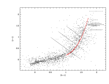
Figure 2: The stars in the five fields in a two color diagram ($(b-r)$ versus $(r-i)$). The spread becomes significant at $(b-r)\geq 1.0$. The solid line is the mean main sequence track, onto which the $(b-r)$ colours of the stars are projected along the $R$ isophotes of varying metallicity (dotted lines). For some extremely red stars, photometric errors are plotted.

This projection implies that stars with $(b-r)_{{\rm corr}}\ga 1.8$ cannot exist in Fig. 3, which shows the spatial distribution of metallicity corrected $(b-r)_{{\rm corr}}$ colors (the limit is indicated by the dashed–dotted line). Both the upper and lower magnitude limits lead to selection effects which have to be taken into account.

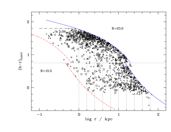
Figure 3: Spatial distribution of metallicity corrected $(b-r)_{{\rm corr}}$. The solid line represents the distance dependent upper color limit at $R=23^{mag}$, the dashed line is the lower limit due to the selection criterium of the fields (no star brighter than $R\approx 15.5$). Since the metal-poor halo stars are intrinsically fainter, the color limits are shifted accordingly. The horizontal line at $(b-r)_{\rm corr}=0.75$ denotes the cut between halo and disk stars in the 13h field (which is why stars can be found ”outside the boundaries”: the color cut is different in each field, see Fig. 1), the dashed–dotted line indicates the cutoff at $(b-r)_{{\rm corr}}=1.8$ due to the metallicity correction. The different symbols refer to the different fields: squares – 1 h field, triangles – 9 h field, dots – 13 h field, open circles – 16 h field, crosses – 23 h field.

4.0.1 Completeness Correction

We correct for incompleteness in the following way (for a detailed derivation of the completeness correction and the corresponding errors we refer the reader to Appendix 1 of Paper I): First, we divide the distance in logarithmic bins of 0.2 and count the stars up to distance dependent color (that is, luminosity) limit, up to which stars can be detected, see Fig. 3. The nearest bins ($-0.8\leq\log r\leq-0.2$) are assumed to be complete. For the incomplete bins we multiply iteratively with a factor given by the ratio of complete to incomplete number counts in the previous bin, where the limit for the uncorrected counts is defined by the bin currently under examination ($j$):

$$N_{j}^{{\rm corr}}=N_{j}\prod_{i=1}^{j-1}(1+\frac{N_{i}^{{}^{\prime\prime}}}{N_{i}^{{}^{\prime}}})\leavevmode\nobreak\ ,$$ (9)

where $N_{j}$ is the number of stars in bin $j$, $N^{{}^{\prime}}$ is the number of stars in the previous bin ($j-1$), up to the limit given by the bin $j$, and $N^{{}^{\prime\prime}}$ is the number of stars from that limit up to the limit given by bin $j-1$.

With the poissonian errors $\sigma_{N}=\sqrt{N}$, $\sigma_{N^{{}^{\prime}}}=\sqrt{N^{{}^{\prime}}}$, and $\sigma_{N^{{}^{\prime\prime}}}=\sqrt{N^{{}^{\prime\prime}}}$ the error of the corrected number counts becomes:

$$\sigma^{2}_{N_{j}^{{\rm corr}}} = \sigma^{2}_{N_{j}}\prod_{i=1}^{j-1}\left(1+\frac{N_{i}^{{}^{\prime\prime}}}{N_{i}^{{}^{\prime}}}\right)^{2}$$ (10)

$$+ \sum_{i=1}^{j-1}\left[\left(\frac{1}{N_{i}^{{}^{\prime}}}\right)^{2}\sigma^{2}_{N_{i}^{{}^{\prime\prime}}}+\left(\frac{N_{i}^{{}^{\prime\prime}}}{N_{i}^{{}^{\prime}}}\right)^{2}\sigma^{2}_{N_{i}^{{}^{\prime}}}\right]$$

$$\cdot \prod_{i=1\atop i\not=j}^{j-1}\left(1+\frac{N_{i}^{{}^{\prime\prime}}}{N_{i}^{{}^{\prime}}}\right)$$

Note that the completeness correction is done for each field separately, thus the different color cuts by which we separate disk from halo stars can be taken into account. Also since the color-magnitude relation is different for disk and halo stars, we calculate the correction factors separately for the two populations. The correction factors are usually in the range $1\leq C\leq 10$, but can be as large as 20 for the last bin of the halo.

With the corrected number counts the density in the logarithmic spaced volume bins ($V_{j}=\frac{1}{3}\omega(r_{j+1}^{3}-r_{j}^{3})$) can then be calculated according to

$$\rho_{j}=\frac{N^{{\rm corr}}_{j}}{V_{j}}=\frac{C\cdot N_{j}}{V_{j}}\leavevmode\nobreak\ ,$$ (11)

For every logarithmic distance bin we use the mean height $z$ above the Galactic plane $<z_{j}>=\sin b\cdot<r>$, where $<\log r>=\log r_{j}+(\log r_{j+1}-\log r_{i})/2=\log r_{i}+0.1\Rightarrow<r>=1.259r_{i}$.

From the estimated density distribution in the five fields we now deduce the structure parameters by fitting the distribution function to the data.

4.1 The distribution of stars in the Galactic disk

We first calculate the density of the stars which we assume to be disk stars, that is, with colors redder than the color cut (see Figure 1 in the field under consideration.

As the nearest stars in our fields have still distances of about 200 pc the normalization at $z=0$ has to be established by other means: We take stars from the CNS4 (Fourth Catalogue of Nearby Stars, Jahreiß & Wielen (1997)), which are located in a sphere with radius 20 pc around the sun. The stars in our normalization sample are selected from the CNS4 by their absolute visual magnitudes, according to the distribution of absolute magnitudes of the CADIS disk stars ($6.5\leq M_{v}\leq 14.5$).

Since the thin disk completely dominates the first kpc and there is no indication of a change of slope within this distance (Fuchs & Wielen 1993), it is justified to fit the density distribution in this range with a single exponential component (taking of course the radial decrease into account). The sum of thick and thin disk stars in the solar neighbourhood, $(n_{1}+n_{2})=6.566\cdot 10^{7}$ kpc^-3 with an uncertainty of 10%, is given by the CNS4 stars. We estimate the scaleheight $h_{1}$ from this fit, assuming two extreme values of the scalelength: $h_{r}=2.0$ kpc, and $h_{r}=3.5$ kpc, respectively (see Table 2). For $h_{r}=2.0$ kpc we find that the weighted mean of the scaleheight of the thin disk is $\overline{h_{1}}=281\pm 13$, for $h_{r}=3.5$ kpc we find $\overline{h_{1}}=283\pm 13$. These values are indistinguishable from each other, and also the values of $\chi^{2}$ indicate that the value adopted for $h_{r}$ does not influence the measurement of the scaleheight $h_{1}$.

Table 2: The scaleheights of the thin disk, assuming a scalelength of $h_{r}=2.0{\rm kpc})$ and $h_{1}(h_{r}=3.5{\rm kpc})$, respectively. The numbers in brackets are the corresponding values of $\chi^{2}$.

CADIS field	$h_{1}(h_{r}=2.0{\rm kpc})$	$h_{1}(h_{r}=3.5{\rm kpc})$
1 h	$249\pm 25$ $(0.92)$	$255\pm 26$ $(0.92)$
9 h	$336\pm 40$ $(1.21)$	$312\pm 35$ $(1.21)$
13 h	$249\pm 24$ $(0.62)$	$255\pm 25$ $(0.63)$
16 h	$321\pm 33$ $(0.41)$	$319\pm 32$ $(0.41)$
23 h	$319\pm 33$ $(1.23)$	$317\pm 33$ $(1.21)$

We then fitted equation (3.1) to the data over the range $0<z<4$ kpc, again for $h_{r}=2.0$ kpc, and $h_{r}=3.5$ kpc, respectively, keeping the corresponding values of $h_{1}$ fixed. With $h_{1}$ and $(n_{1}+n_{2})$ known, the free parameters are now the scaleheight $h_{2}$ of the thick disk, and the ratio $n_{2}/(n_{1}+n_{2})$. Again the measurement is insensible to the scalelength assumed in equation (3.1). This is due to the high Galactic latitude of the CADIS fields ($45\leq b\leq 60$) – the halo becomes dominant already at a projected radial distance of only about $7$ kpc.

Although the number of degrees of freedom is already kept to a minimum, this fit is highly degenerated, as can be seen from the $\chi^{2}$ distribution (see Fig. 4), where we asumed $h_{r}=3.5$ kpc. The contour lines show the $1$,$2$ and $3\sigma$ confidence levels. Neither the ratio $n_{2}/(n_{1}+n_{2})$ nor the value of the scaleheight of the thick disk can be estimated with high accuracy. Except for the 9 h field, where the $\chi^{2}$ distribution suggests a very large value of $h_{2}$, the minimum can be found at around $900\la h_{2}\la 1100$ kpc, and $n_{2}/(n_{1}+n_{2})\la 0.05$. The fit of the scaleheight of the thick disk in the 9 h field is mainly influenced by the one data point at $z\approx 3.6$ kpc, where the density seems to be extraordinarily high. Because this value appears to be an exception, we disregard it in the calculation of the mean. The mean $\chi^{2}$, excluding the 9 h field, is $h_{2}\approx 1000$, $n_{2}/(n_{1}+n_{2})\approx 0.04$. Including the 9 h field, the mean $\chi^{2}$ (lower right corner) is approximately at $h_{2}\approx 1200$, $n_{2}/(n_{1}+n_{2})\approx 0.04$.

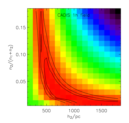
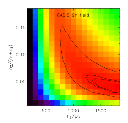
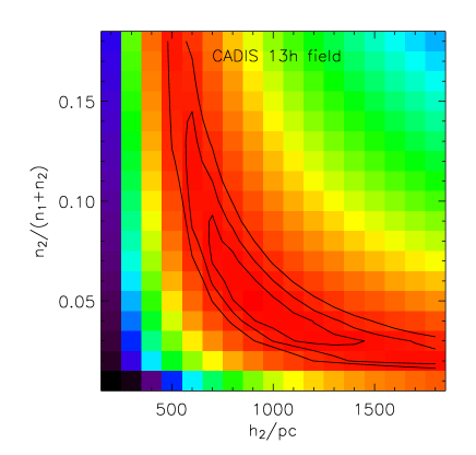
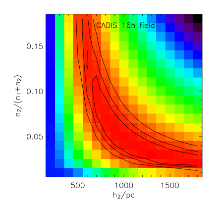
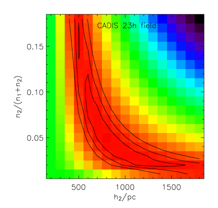
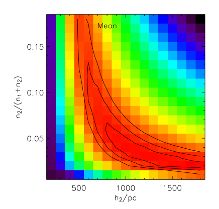
Figure 4: $\chi^{2}$ plane for the parameters $h_{2}$ and $n_{2}/(n_{1}+n_{2})$ for the fit of the measured density distribution in the five fields, and the mean $\chi^{2}$ of all five ones (bottom right). The scalelength is assumed to be $h_{r}=3.5$ kpc, and the values of $h_{1}$ are given in Table 2. The contour lines show the $1\sigma$,$2\sigma$ and $3\sigma$ confidence levels.

Figure 5 shows the density distribution of the disk stars in the five fields, and the corresponding best fits. The value for the local normalisation is given by the CNS4, and the values for $h1$ can be found in Table 2 (we assumed $h_{r}=3.5$ kpc). The fraction of thick disk stars in the local normalisation is assumed to be $n_{2}/(n_{1}+n_{2})=0.04$, and the mean value of $h_{2}=1.0$ kpc was adopted for all fields except for the 9 h field, where a formal value of $h_{2}=2.6$ kpc is required to achieve a satisfying fit.

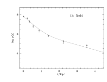
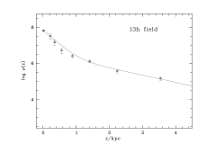
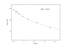
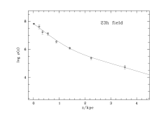
Figure 5: Density distribution of the stars in the disk. The solid line is the best fit for a sum of two exponentials.

4.2 The stellar density distribution of the Galactic halo

For the local normalisation we take stars from the CNS4, which have been discriminated against disk stars by their metallicities and kinematics (Fuchs & Jahreiß 1998). From these we selected stars with $-0.2\leq(b-r)\leq 0.7$ (which corresponds to $3.5\leq M_{V}\leq 7.5$). All these stars have very low metallicities ($\left[Fe/H\right]<-1$ dex) and large space velocities (see Table 1 in Fuchs & Jahreiß (1998)), which clearly identifies them as halo stars. The following six stars in a radius of $r\leq 23$ pc around the sun satisfy the criteria: Gl 53A, Gl 451A, Gl 158A, GJ 1064A, GJ1064B, LHS 2815. Thus we find $\rho_{0}=89125\pm 35650$  stars/kpc³.

Fig. (6) shows the completeness corrected density distribution of all stars. We fitted equation (5) to the last four data points, while keeping the normalisation at $z=0$ fixed to the value given by the stars from the CNS4. We estimated the power law index $\alpha$ for a flattened halo with an axis ratio of $c/a=0.6$ (dashed line in Fig. (6)), and no flattening ($c/a=1.0$, solid line). The values of $\alpha$ we deduced from the fit to the data are listed in Table 3.

Table 3: The exponent $\alpha$ from equation (5), for a flattened halo with an axis ratio of $c/a=0.6$, and for $c/a=1.0$ (no flattening). The numbers in brackets are the corresponding $\chi^{2}$ values.

CADIS field	$\alpha(c/a=0.6)$	$\alpha(c/a=1.0)$
1 h	$2.36\pm 0.14(1.37)$	$2.8\pm 0.16(1.05)$
9 h	$0.44\pm 0.08(13.99)$	$0.5\pm 0.1(13.68)$
13 h	$1.50\pm 0.09(3.13)$	$1.98\pm 0.09(1.54)$
16 h	$2.84\pm 0.14(3.24)$	$3.52\pm 0.18(1.65)$
23 h	$2.98\pm 0.18(11.81)$	$3.68\pm 0.22(7.01)$

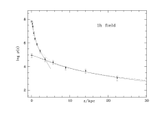
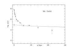
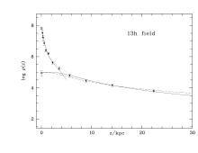
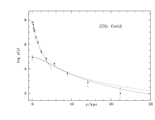
Figure 6: Density distribution of all stars. The solid lines are the best fits for the disk (as in Figure (5)) and a spherical halo, the dashed line is the fit for a flattened halo with axial ratio $(c/a)=0.6$. The corresponding exponents $\alpha$ are given in Table (3)). The dotted line is the sum of disk and spherical halo (which is slightly favoured by the fit).

Clearly the fit in the 9 h field is dominated by one exceptionally high data point at $z\approx 10$ kpc, and does not give a reliable result. The weighted mean, disregarding the 9 h field, is $\alpha=2.12\pm 0.06$ for $(c/a)=0.6$, and $\alpha=2.51\pm 0.07$ for $(c/a)=1.0$, where the $\chi^{2}$ values favour a halo without strong flattening: The sum of the $\chi^{2}$ values of the fits in the four single fields which enter in the determination are $\sum{\chi^{2}}=19.55$ for the flattened, and $\sum{\chi^{2}}=11.25$ for the spherical halo.

The axis ratio assumed for the estimation of the power law index $\alpha$ influences the fitted value: the flatter the halo, the smaller $\alpha$. But not only the axial ratio influences the measurement of $\alpha$, also the local normalisation adopted for the fit. In order to estimate the effect we fitted the data for $\rho_{0}^{\rm uplim}=\rho_{0}+\sigma_{\rho_{0}}$ and $\rho_{0}^{\rm lowlim}=\rho_{0}-\sigma_{\rho_{0}}$, respectively, and found weighted means of $\alpha(\rho_{0}^{\rm uplim})=2.26\pm 0.05$ (with $\sum{\chi^{2}}=10.82$) and $\alpha(\rho_{0}^{\rm lowlim})=1.68\pm 0.07$ ($\sum{\chi^{2}}=51.29$) for $(c/a)=0.6$, and $\alpha(\rho_{0}^{\rm uplim})=2.95\pm 0.07$ ($\sum{\chi^{2}}=16.45$) and $\alpha(\rho_{0}^{\rm lowlim})=1.97\pm 0.07$ ($\sum{\chi^{2}}=30.12$) for $(c/a)=1.0$, respectively (again leaving out the 9 h field).

The values of $\alpha$ are getting larger for a larger value of $\rho_{0}$, and smaller for smaller $\rho_{0}$. However, the the summed $\chi^{2}$ indicate that the normalisation given by the CNS4 stars is not too far away from the ”true” normalisation. The true value is definitely not smaller. If it is slightly larger, then a flattened halo is favoured. However, it is not possible to measure the flattening of the halo accurately with the current data set.

4.3 The stellar luminosity function of the disk

Knowing the density distribution of the thin disk stars, we can calculate the stellar luminosity function $\Phi(M_{V})$. We restrict the analysis to stars within a radius of $r\leq 1.5$ kpc, for beyond this range the contribution by thick disk and halo stars becomes dominant. As in Paper I, we calculate absolute visual magnitudes from the $R$ magnitudes to make comparison with literature easier. In the relevant magnitude intervall ($5\leq M_{V}\leq 14$, i.e $-1<(b-r)<1.8$) there holds an empirical linear relation:

$$M_{V_{J}}=1.058\cdot M_{R_{C}}\leavevmode\nobreak\ .$$ (12)

For every luminosity bin the effective volume is calculated by integrating the distribution function along the line of sight, $r$, where the integration limits are given by the minimum between 1.5 kpc and the distance modulus derived for upper and lower limiting apparent magnitude:

$$V_{{\rm max}}^{{\rm eff}}=\omega\int\limits_{R_{{\rm min}}}^{R_{{\rm max}}}\nu(r,b)\leavevmode\nobreak\ r^{2}\leavevmode\nobreak\ dr\leavevmode\nobreak\ ,$$ (13)

where

$$R_{{\rm min}} = 10^{0.2(16^{{\rm mag}}-M_{R})-2.0}\leavevmode\nobreak\ ,$$

$$R_{{\rm max}} = {\rm min}(1.5\leavevmode\nobreak\ {\rm kpc},10^{0.2(23^{{\rm mag}}-M_{\rm R})-2.0})\leavevmode\nobreak\ .$$

The distribution function

$$\nu(r,b)=\exp(-r\sin b/h_{1})$$ (14)

is normalised to unity at $z=0$.

The weighted mean of the SLFs of the five CADIS fields is shown in Fig. 7. For each single field we also calculated the effective volume by using the measured values of $h_{1}$. Also shown in Fig. 7 are the SLFs one would measure for $h_{1}=0.250$ kpc and $h_{1}=0.350$ kpc (dotted and dashed lines in the upper panel), in order to demonstrate how the SLF changes with the scaleheight assumed for the calculation of the effective volume. The dash-dotted line in the middle shows our old determination as published in Paper I (Fig. 10), the dashed line is the local SLF (Jahreiß & Wielen 1997) of stars inside a radius of 20 pc around the sun, which is based on HIPPARCOS parallaxes. In the range where the SLFs overlap, they are consistent with each other. As in Paper I we calculated the weighted mean of CADIS and local SLF, which is shown in the lower panel of Fig. 7, in comparison with a photometric SLF which is based on HST observations (Gould et al. 1998).

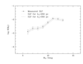
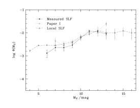
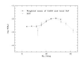
Figure 7: Upper panel: the mean SLF of the five CADIS fields (solid line). For the calculation of the effective volumes we used the fitted values of $h_{1}$ (see Table 2). The dotted and dashed lines are the determination for $h_{1}=0.250$ kpc, and for $h_{1}=0.350$ kpc, respectively. Middle panel: The solid line is our current measurement, as in the upper panel. The dotted line is our first measurement as published in Paper I, the dashed line is the local SLF (Jahreiß & Wielen 1997), which is based on HIPPARCOS parallaxes. Lower panel: weighted mean of CADIS and local SLF, in comparison with a photometric SLF which is based on HST observations (Gould et al. 1998).

We will use this luminosity function as input for the simulation, which we describe in the following section.

5 A Monte Carlo model of the Milky Way

The method described in the previous section has the disadvantage that it involves a completeness correction, since faint stars can only be traced at small distances. However, it is possible to avoid completeness corrections, by modeling the observed colors and apparent magnitudes of the stars in the fields, using Monte Carlo simulations. The best-fitting model of the Galaxy can be determined by $\chi^{2}$-fitting or a maximum likelihood analysis.

The two basic incredients are the stellar density distribution function and the stellar luminosity function. We will keep the luminosity function fixed, while varying the structure parameters of the density distribution.

5.1 The Density Distribution

We use the same model of the Milky Way as described in Section (3): a sum of two exponential disks with scaleheights $h_{1}<h_{2}$, and a power law halo.

The local density is again given by the CNS4 stars (Jahreiß & Wielen 1997; Fuchs & Jahreiß 1998). The contribution of thick disk stars to the local normalisation, $n_{2}/(n_{1}+n_{2})$, is left as a free parameter, and is varied from 2% to 18% in steps of $1$ %. The scaleheights $h_{1}$ and $h_{2}$ are varied from $150$ pc to $400$ pc in steps of $50$ pc, and from $200$ pc to $1800$ pc in steps of $100$ pc, respectively. The simulation was run for a radial scalelength $h_{r}=2000$ pc, and for $h_{r}=3500$ pc. The power law index of the stellar halo was increased from $\alpha=2.0$ to $\alpha=4.0$ in steps of $0.5$, for a spherical as well as for a flattened halo with an axis ratio $(c/a)=0.6$.

For each field, the expected number of stars $N$ in the model under consideration is calculated by integrating the distribution function along the line of sight:

$$N=\int_{0}^{\infty}{\rho(r,l,b)\leavevmode\nobreak\ \omega r^{2}}{\mathrm{d}}r\leavevmode\nobreak\ ,$$ (15)

where $\omega=7.6145\cdot 10^{-6}$ for one CADIS field and $\rho(r,l,b)=\rho(r,l,b)_{\rm disk}+\rho(r,l,b)_{\rm halo}$. For each of the $24\,480$ combinations of structure parameters we simulated $1000$ times more stars than observed in each CADIS field, in order to avoid large poisson noise in the model data.

5.2 Magnitudes and colors

In order to simulate “observed” apparent magnitudes and colors and to keep the two different approaches consistent, we have essentially to invert the steps described in Section 4. First of all each star which has been simulated according to the density distribution function is assigned an absolute magnitude following the stellar luminosity function determined from our sample (see Section 4.3). The faint end of the luminosity function of halo stars has only been determined with high uncertainties (Gould 2003). Although it has been suggested that the luminosity function of the halo stars might be different from the one of the disk stars (Reylé & Robin 2001), there is no accurate measurement available: The measurement of the luminosity function of halo subdwarfs is extremely sensible to the distance range in which it is determined – the SLFs measured from local subdwarfs (where the number of stars is very small and limits the accuracy of the measurement) differ from those measured in the outer halo. The reason for these discrepancies might be the insufficient accuracy with which the stellar structure of the halo is known (Digby et al. 2003). Therefore, as long as the the luminosity function is not determined with higher accuracy and the density distribution of the halo is known better, we use our measured SLF for both disk and halo stars.

In the range $6\leq M_{V}\leq 13$ the mean of the measured CADIS and the local SLF from Jahreiß & Wielen (1997) can be described quite precisely by a third-order polynomial in log-space:

$$\log\Phi(M_{V})=\sum_{i=0,3}c_{i}M^{i}\leavevmode\nobreak\ ,$$ (16)

with $c_{0}=4.78676$, $c_{1}=-2.63075$, $c_{2}=0.297266$, $-0.0104039$.

Each star is assigned an absolute $V$ band luminosity, randomly chosen from a distribution following equation (16). Since there is no $V$ or comparable filter available in the CADIS filter set, we have to convert the $M_{V}$ magnitudes into $M_{R_{C}}$ magnitudes (see Paper I), i.e. $M_{R_{C}}=0.945\cdot M_{V}$. CADIS $(b-r)_{C}$ colors can be calculated from the absolute $R_{C}$ band magnitudes using the main sequence relation described in Paper I. The same relation was used in Section 4 to deduce absolute magnitudes from the $(b-r)_{C}$ colors of the stars.

5.2.1 Metallicities

In Section 4 we have corrected for the influence of different metallicities on the color-magnitude relation. Now we have to simulate those effects in order to compare the model with the data. Halo stars are again assumed to be fainter by $\Delta M_{R}=0.75$ as disk stars of the same color. In the direct determination we have not been able to separate thin from thick disk stars. In the simulation however, we can account for the fact that thick disk stars have subsolar metallicities, and hence have a different color-magnitude relation than thin disk stars with solar metallicities. From a sample of 5 thick disk stars with $-0.3<\left[{\rm Fe/H}\right]<-0.95$, where HIPPARCOS parallaxes, spectroscopic metallicities and photometry in blue and red passbands are available, we estimate the offset from the solar main sequence valid for the thin disk stars to be $\Delta M_{R}\approx 0.35$ (C. Flynn, priv.comm.).

In order to take the spread in metallicities into account, the simulated colors are then smeared out by adding a value taken from a uniform distribution of numbers in the range $-0.2\leq\delta(b-r)\leq+0.2$.

5.2.2 Photometric errors

Our observed data have of course photometric errors, which are of the order of $\sigma_{R}=0.01$ in case of the brighter ($R\leq 21$) and $\sigma_{R}=0.15$ for the faintest ($R\approx 23$) stars. These have to be simulated as well, in order to allow for a reliable comparison with the observations. Using the distance modulus $m-M=5\log r-5$, the apparent magnitudes of the stars are calculated. Each star is assigned a photometric error which is chosen randomly out of a gaussian error distribution with a variance corresponding to its apparent magnitude. The error is added to the apparent $R$ magnitude. The procedure is repeated for the $B$ magnitudes, which have been calculated from the simulated $(b-r)_{C}$ colors. The final colors are then redetermined from the new, modified magnitudes.

5.3 “Observing” the Model

Each simulated star has now an apparent $R_{C}$ magnitude and a $(b-r)_{C}$ color, where metallicity effects and photometric errors are incorporated in the simulation. These data can now be compared with the observed data.

The simulated stars are selected by their apparent magnitudes ($15.5\leq R_{C}\leq 23$). We bin the data, observed and simulated, into a grid with steps of $\Delta R_{C}=0.5$ in magnitude and $\Delta(b-r)_{C}=0.2$ in color.

Due to our survey selection criteria the bins at bright apparent magnitudes contain only very few stars, which makes a $\chi^{2}$ fit of the model to the data extremely difficult. Instead of using $\chi^{2}$ as an estimate of the goodness of fit, we use the C-statistic for sparse sampling, which was developed by Cash (1979). It is based on the likelihood ratio, and is suited for small number statistics. In the limit of large numbers it converges to $\chi^{2}$.

If $n_{i}$ is the number of stars in the bin, $e_{i}$ the expectation value predicted by the model and $N$ the number of bins, then

$$C=\frac{2}{N}\sum_{i=1}^{N}{\left[n_{i}\ln\left(\frac{n_{i}}{e_{i}}\right)-(n_{i}-e_{i})\right]}$$ (17)

For each of the $24\,480$ models of each field we calculate $C$ by summing over the bins in the magnitude-color grid.

The overall $C$ is lowest for $\alpha=2.5$, $(c/a)=0.6$, $h_{r}=3500$ pc, and $h_{1}=300$ pc, while $C$ is only marginally larger if $(c/a)=1.0$ (and $\alpha=3.0$). There is no significant difference between models with $h_{r}=2000$ pc or $h_{r}=3500$ pc. This is consistent with the results from the previous section. Figure (8) shows the $C$ planes for $h_{2}$ and $n_{2}/(n_{1}+n_{2})$ (with $h_{r}=3500$ pc, $h_{1}=300$ pc, $(c/a)=0.6$, and $\alpha$ fixed at $2.5$), for each of the five individual fields and the mean of all of them.

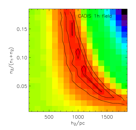
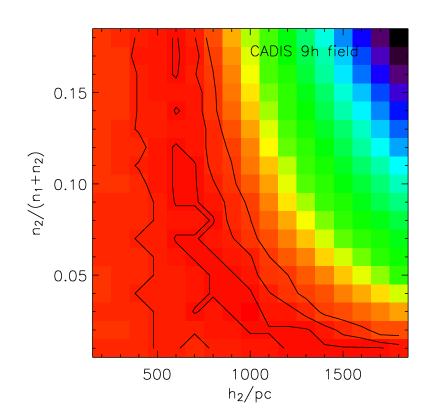
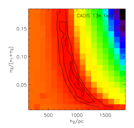
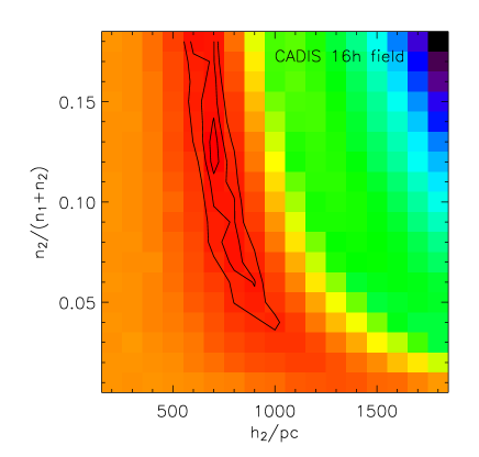
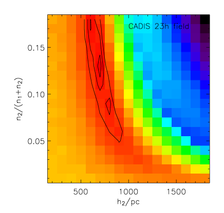
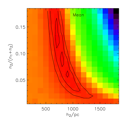
Figure 8: The $C$ planes of the five fields for the parameter $h_{2}$ and $n_{2}/(n_{1}+n_{2})$ (with $h_{r}=3500$ pc, $h_{1}=300$ pc, $(c/a)=0.6$,and $\alpha=2.5$). The plot in the lower right corner is the mean of the five indidual fields. The contour lines show the $1\sigma$, $2\sigma$, and $3\sigma$ confidence levels.

From the mean of the five fields we find the minimum of the $C$ statistic to be at $h_{2}=900$ pc and $n_{2}/(n_{1}+n_{2})\approx 0.09$. While the value of $h_{2}$ is consistent with the value derived from the direct measurement, the relative normalisation is higher. However, the fit is highly degenerated, and the minimum in the distribution of $C$ is streched along the $n_{2}/(n_{1}+n_{2})$-axis. Thus the relative normalisation is only measurable with extremely large errors, and the rather high value of $n_{2}/(n_{1}+n_{2})=0.09$ should be regarded as an upper limit.

Figure (9) shows the color-coded representation of the density of the stars in the magnitude-color diagram for the five fields. The images have been rebinned in steps of $0.1$ in both color and magnitude. The contour plots overlaid are the simulated best-fit cases of the model ($h_{r}=3500$ pc, $h_{1}=300$ pc, $h_{2}=900$ pc, $n_{2}/(n_{1}+n_{2})=0.09$, $(c/a)=0.6$ and $\alpha=2.5$).

The prominent structure at the left of each image consists of disk stars, whereas the halo stars are mainly distributed at the right. The simulation matches the data very well except for the 13 h field, where the gap between halo and disk is not modelled. In all cases the halo does not match the data very well, a possible explanation might be that the real halo luminosity function, which we do not know, is in fact significantly different from the disk luminosity function which we use for the simulation.

\begin{picture}(21.0,25.0)\put(1.0,17.0){\epsfbox{colormagtest_01.ps}} \put(1.0,9.0){\epsfbox{colormagtest_13.ps}} \put(9.0,17.0){\epsfbox{colormagtest_09.ps}} \put(9.0,9.0){\epsfbox{colormagtest_16.ps}} \put(1.0,1.0){\epsfbox{colormagtest_23.ps}} \end{picture}

Figure 9: The number density of stars in the $(b-r)_{C}$-$R_{C}$ plane, for the five fields. The densities are normalised to the total number of stars in each field. The images have been rebinned in steps of $0.1$ in both color and magnitude. The contours overlaid are the simulated data for $h_{r}=3500$ pc, $h_{1}=300$ pc, $h_{2}=900$ pc, $n_{2}/(n_{1}+n_{2})=0.09$, $(c/a)=0.6$ and $\alpha=2.5$, also normalised to the number of simulated stars. The contours are plotted for $0.001\leq N\leq 0.015$ in steps of $0.001$.

Figure (10) shows the distribution of absolute $V$ band magnitudes of the CADIS data (calculated from the $(b-r)_{C}$ colors as described in Section 5.2) in comparison with the simulated data, for the best fit cases. Both histograms have been normalised to the total number of stars, in order that they can be compared directly.

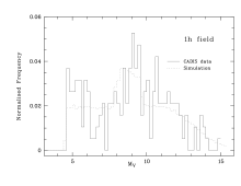
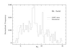
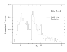
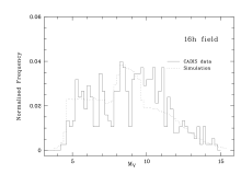
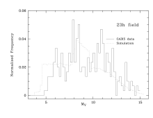
Figure 10: Comparison of absolute $V$ band magnitudes of the simulation (dotted line) with the CADIS data (solid line), for the best fit case.

With exception of the CADIS 23 h field the distribution of absolute $V$ band magnitudes is matched very well by the simulation. In the 9 h field the model can not account for the large peak at $M_{V}\sim 8$. It is not improbable that the Galactic halo is clumpy (Newberg et al. 2002), so the the feature may well be an overdensity of stars with respect to the smooth powerlaw halo.

In the 23 h field the number of bright halo stars is overpredicted. Since the 16 h and the 23 h fields are located at the same Galactic longitude and $|b_{16h}|\approx|b_{23h}|$, both fields should show the same distribution of color or absolute magnitudes, respectively. However, as both distributions differ from each other at the bright end, it seems more likely that the 23 h field is ’missing’ some stars, rather than that the model (which matches the 16 h field more closely) overpredicts stars which are not supposed to be there.

6 Summary and Discussion

Our model of the Galaxy consists of three components: a thin and a thick disk (described by a sum of two exponentials), and a power law halo. The local normalisation of disk and halo stars has been fixed by stars selected from the CNS4 (Jahreiß & Wielen 1997) by their colors and apparent magnitudes.

We have estimated the structure parameters of the stellar density distribution of the Milky Way using two different, complementary methods: from a direct measurement of the density distribution of stars perpendicular to the Galactic plane (Baconian ansatz), and by modelling the observed colors and apparent magnitudes of the stars and comparing them to the data (Kartesian ansatz).

Both methods have their advantages and limitations: the direct determination of the density involves completeness corrections because faint stars are only traced to small distances. These rely on the assumption that the stellar luminosity function (SLF) does not change with distance and is the same for disk and halo stars. The same assumption of course is used in the simulation. However, the simulation avoids completeness corrections and thus the errors do not depend on an iterative correction. A $\chi^{2}$ fitting of a simulated color-magnitude distribution of stars works very well for a large number of stars; with the CADIS data the method is at the edge of feasibility. We therefore used the $C$ statistic developed by Cash (1979) for sparse sampling to find the best fitting parameter combination.

From the $\chi^{2}$ fit to the direct measurement of the density distribution of the stars, we find $h_{1}=281\pm 13$ pc if we assume $h_{r}=2000$ pc, and $h_{1}=283\pm 13$ pc if $h_{r}=3500$ pc. Obviously, due to the high Galactic latitude of the fields ($45\leq b\leq 60$), we are not able to measure the scalelength (the halo becomes dominant already at a projected radial distance of only about 7 kpc). The fit of the scaleheight of the thick disk and the local percentage of thick disk stars is highly degenerate. The best estimate is $h_{2}\approx 1000$ kpc, and $n_{2}/(n1+n_{2})\approx 0.04$. We also fitted the density distribution in the halo and find $\alpha=2.51\pm 0.07$ for $(c/a)=1.0$, and $\alpha=2.12\pm 0.06$ if we allow for a flattening of the stellar halo with an axial ratio of $(c/a)=0.6$. The values of $\chi^{2}$ formally favour the spherical halo, but this result is not significant, since the power law slope and the axial ratio are highly correlated. Furthermore the measured values of the exponent $\alpha$, and the axial ratio $c/a$ depend on the local normalisation assumed for the fit: slightly higher (lower) values of $\rho_{0}$ yield slightly higher (lower) values of $\alpha$, and a flattened (spherical) halo is favoured.

From the Cartesian method we derive $h_{2}\approx 900$ kpc, $n_{2}/(n1+n_{2})\approx 0.09$. We also find that the overall $\chi^{2}$ or $C$, respectively, is smallest for $h_{1}=300$ pc and an exponent $\alpha=3.0$. If we allow for a flattening of the halo with an axial ratio of $(c/a)=0.6$, we find that a slightly smaller value of $\alpha=2.5$ fits the data better. The corresponding values of $\chi^{2}$ or $C$, respectively, are only marginally smaller for a flattened halo. The values of $\alpha$ are generally slightly larger than in the direct measurement. A possible explanation for this difference is that when we fit the simulated distribution of stars in the color-magnitude diagram, we fit all components of the galaxy simultaneously (whereas in the direct measurement we fit disk and halo separately), and there might be a degeneracy between halo and thick disk parameters.

However, in general both methods yield essentially the same result, which we regard as a corroboration that both work correctly within their limitations.

6.1 Comparison with other results

A very detailed compilation of different results from different authors can be found in Siegel et al. (2002). The values for the scaleheight of the thick disk and the relative normalisation of thick disk stars range from 900 kpc to 2400 kpc, and from 1 % to 6 %, respectively.

Chen et al. (2001) carried out an investigation of Galactic structure using $5.8\cdot 10^{5}$ stars brighter than $g^{\prime}=21^{\rm mag}$ from the Sloan Digital Sky Survey (SDSS), covering a total area of 279  ^∘. They presented models of the Milky Way for a large number of free parameters, that is, they determine by means of a maximum likelyhood analysis the scaleheights of the thin and thick disk, respectively, the relative normalisation of both disk components in the solar neighbourhood, the offset of the sun above the Galactic plane, the exponent $\alpha$ of the power law halo and the flattening of the halo.

They find $h_{1}=330\pm 3$ pc, $580\la h_{2}\la 750$ pc, $0.065\la n_{2}/(n_{1}+n_{2})\la 0.13$, and $\alpha=2.5\pm 0.3$, and $c/a=0.55\pm 0.06$. Lemon et al. (2004) also found a significant flattening of the halo ($c/a=0.56\pm 0.01$).

While our results lie well within the range found by most authors, our measurements for the scaleheights of the disk are quite dissimilar from the Sloan results.

A possible explanation might be that their determination, the results of which differ significantly from all other determinations, suffers from the degeneracy due to the large number of degrees of freedom in their simulation: their fitting routine may have found a secondary minimum.

Robin et al. (2000) found that there is a significant degeneracy between the power law index $\alpha$ and the axis ratio of the halo. Their best fit to the data yields $\alpha=2.44$ and $c/a=0.76$, but a flatter spheroid with $c/a=0.6$ with $\alpha=2$ is not excluded either. We find the same degeneracy in our data: If we assume $(c/a)=0.6$, we find $\alpha=2.12\pm 0.06$ (or $\alpha=2.5$ in the simulation), whereas for $(c/a)=1.0$ we find that $\alpha=2.51\pm 0.07$ ( $\alpha=3.0$) fits the data better.

6.2 Future prospects

This investigation shows quite clearly that the fit of a sum of two exponentials is highly degenerate if the relative normalisation $n_{2}/n_{1}$ or the scaleheights $h_{1}$ and $h_{2}$ is not known. Also the measurement of $\alpha$, the power law index of the stellar halo, and its axial ratio, $(c/a)$, are correlated and depend on the local normalisation.

Therefore it certainly depends on the assumptions and the number of the degrees of freedom which values of $h_{1}$, $h_{2}$, $n_{1}$, $n_{2}$, $\alpha$, and $(c/a)$ are determined in different analyses. The more structure parameters are known and kept fixed, the narrower is the $\chi^{2}$ (or $C$) distribution. Thus it is important to combine results from different methods.

The scaleheight of the thick disk for example will be determinable with high accuracy if the local normalisation of thick disk stars is known better. The local density of stars belonging to different components of the Galaxy has to be determined by means of kinematics and metalicities of the stars in order to break the degeneracy of the fit of a double exponential.

The degeneracy between the power law slope and the flattening of the halo can be broken by simultaneously fitting density distributions estimated from deep star counts in a large number of fields at different Galactic latitudes and longitudes, respectively.

When the “size” and exact shape of the stellar halo is known, it will become much easier to determine the structure parameters of the thick disk.

CADIS, although designed as an extragalactic survey, provided a sufficient number of stars (and fields) to investigate the structure of the Milky Way. However, not only larger statistics, but also a much better knowledge of the luminosity function of halo stars is required to increase the accuracy of the results.

References

- Bahcall & Soneira (1980a) Bahcall, J. N. & Soneira, R. M. 1980a, ApJ, 238, L17
- Bahcall & Soneira (1980b) —. 1980b, ApJS, 44, 73
- Bahcall & Soneira (1981) —. 1981, ApJS, 47, 357
- Bertin & Arnouts (1996) Bertin, E. & Arnouts, S. 1996, A&AS, 117, 393
- Bienaymé (1999) Bienaymé, O. 1999, A&A, 341, 86
- Cash (1979) Cash, W. 1979, ApJ, 228, 939
- Chen et al. (1999) Chen, B., Figueras, F., Torra, J., et al. 1999, A&A, 352, 459
- Chen et al. (2001) Chen, B., Stoughton, C., Smith, J. A., et al. 2001, ApJ, 553, 184
- Digby et al. (2003) Digby, A. P., Hambly, N. C., Cooke, J. A., Reid, I. N., & Cannon, R. D. 2003, MNRAS, 344, 583
- Freeman (1992) Freeman, K. C. 1992, in IAU Symp. 149: The Stellar Populations of Galaxies, 65
- Fried et al. (2001) Fried, J. W., von Kuhlmann, B., Meisenheimer, K., et al. 2001, A&A, 367, 788
- Fuchs & Jahreiß (1998) Fuchs, B. & Jahreiß, H. 1998, A&A, 329, 81
- Fuchs & Wielen (1993) Fuchs, B. & Wielen, R. 1993, in AIP Conf. Proc. 278: Back to the Galaxy, 580
- Gilmore (1984) Gilmore, G. 1984, MNRAS, 207, 223
- Gilmore & Reid (1983) Gilmore, G. & Reid, N. 1983, MNRAS, 202, 1025
- Gilmore & Wyse (1987) Gilmore, G. & Wyse, R. F. G. 1987, in NATO ASIC Proc. 207: The Galaxy, 247–279
- Gould (2003) Gould, A. 2003, ApJ, 583, 765
- Gould et al. (1998) Gould, A., Flynn, C., & Bahcall, J. N. 1998, ApJ, 503, 798
- Jahreiß & Wielen (1997) Jahreiß, H. & Wielen, R. 1997, Proceedings of the ESA Symposium ‘Hipparcos - Venice ’97’, 13-16 May, Venice, Italy, ESA SP-402 (July 1997), p. 675-680, 402, 675
- Lang (1992) Lang, K. R. 1992, in Astrophysical Data I. Planets and Stars, X, 937 pp. 33 figs.. Springer-Verlag Berlin Heidelberg New York
- Lemon et al. (2004) Lemon, D. J., Wyse, R. F. G., Liske, J., Driver, S. P., & Horne, K. 2004, MNRAS, 347, 1043
- Meisenheimer & Röser (1986) Meisenheimer, K. & Röser, H.-J. 1986, in Use of CCD Detectors in Astronomy, Baluteau J.-P. and D’Odorico S., (eds.), 227
- Mendez & van Altena (1998) Mendez, R. A. & van Altena, W. F. 1998, A&A, 330, 910
- Newberg et al. (2002) Newberg, H. J., Yanny, B., Rockosi, C., et al. 2002, ApJ, 569, 245
- Norris (1999) Norris, J. E. 1999, Ap&SS, 265, 213
- Ojha et al. (1996) Ojha, D. K., Bienayme, O., Robin, A. C., Creze, M., & Mohan, V. 1996, A&A, 311, 456
- Oke (1990) Oke, J. B. 1990, AJ, 99, 1621
- Phleps et al. (2000) Phleps, S., Meisenheimer, K., Fuchs, B., & Wolf, C. 2000, A&A, 356, 108
- Pickles (1998) Pickles, A. J. 1998, PASP, 110, 863
- Reid et al. (1997) Reid, I. N., Gizis, J. E., Cohen, J. G., et al. 1997, PASP, 109, 559
- Reid et al. (1996) Reid, I. N., Yan, L., Majewski, S., Thompson, I., & Smail, I. 1996, AJ, 112, 1472
- Reid & Majewski (1993) Reid, N. & Majewski, S. R. 1993, ApJ, 409, 635
- Reylé & Robin (2001) Reylé, C. & Robin, A. C. 2001, A&A, 373, 886
- Robin & Creze (1986) Robin, A. & Creze, M. 1986, A&A, 157, 71
- Robin et al. (1992) Robin, A. C., Creze, M., & Mohan, V. 1992, A&A, 265, 32
- Robin et al. (2000) Robin, A. C., Reylé, C., & Crézé, M. 2000, A&A, 359, 103
- Röser & Meisenheimer (1991) Röser, H. . & Meisenheimer, K. 1991, A&A, 252, 458
- Ruphy et al. (1996) Ruphy, S., Robin, A. C., Epchtein, N., et al. 1996, A&A, 313, L21
- Siegel et al. (2002) Siegel, M. H., Majewski, S. R., Reid, I. N., & Thompson, I. B. 2002, ApJ, 578, 151
- Wainscoat et al. (1992) Wainscoat, R. J., Cohen, M., Volk, K., Walker, H. J., & Schwartz, D. E. 1992, ApJS, 83, 111
- Walsh (1995) Walsh, J. 1995, http://www.eso.org/observing/standards/spectra
- Wolf et al. (2001a) Wolf, C., Meisenheimer, K., & Röser, H. . 2001a, A&A, 365, 660
- Wolf et al. (2001b) Wolf, C., Meisenheimer, K., Röser, H. ., et al. 2001b, A&A, 365, 681
- Young (1976) Young, P. J. 1976, AJ, 81, 807