Fitting Photometry of Blended Microlensing Events

Abstract

We reexamine the usefulness of fitting blended lightcurve models to microlensing photometric data. We find agreement with previous workers (e.g. Woźniak & Paczyński ) that this is a difficult proposition because of the degeneracy of blend fraction with other fit parameters. We show that follow-up observations at specific point along the lightcurve (peak region and wings) of high magnification events are the most helpful in removing degeneracies. We also show that very small errors in the baseline magnitude can result in problems in measuring the blend fraction, and study the importance of non-Gaussian errors in the fit results. The biases and skewness in the distribution of the recovered blend fraction is discussed. We also find a new approximation formula relating the blend fraction and the unblended fit parameters to the underlying event duration needed to estimate microlensing optical depth.

1 Introduction

Gravitational microlensing has become a useful tool in measuring the amount of matter along the line-of-sight to distant stars. Since gravitational lensing depends only on mass, microlensing is sensitive to all compact forms of matter independent of their luminosity. Thus measurements out of the plane of the Galaxy towards the LMC, SMC, and M31 have given important limits/detections of dark matter in the halo ( Aubourg, et al.  1993; Lasserre et al.  2000; Alcock, et al. 1993; 1997a; 2000; Paulin-Henriksson et al. 2003; de Jong et al. 2004), and measurements towards the Galactic bulge give important constraints on the mass and distribution of Galactic stars, including those too faint to observe directly (Griest et al. 1991; Paczyński 1991; Han & Gould 2003; Udalski, et al. 1994; Alcock, et al. 1997b; Afonso, et al. 2003; Popowski, et al. 2005; Sumi, et al. 2005).

The signal of microlensing is a specific transient magnification of a background source star as the lens object passes in front of it, and thus microlensing experiments repeatedly monitor many ordinary stars to find microlensing lightcurves. The probability of microlensing occurring to a given star is called the optical depth, $\tau$ and is of order $10^{-6}$ or less for many Milky Way lines-of-sight. The smallness of $\tau$ means that microlensing experiments concentrate on very crowded star fields where many hundreds of thousands of stars can be simultaneously imaged. This allows many lightcurves to be created simultaneously but also results in blending of the source stars together. This blending causes two problems in using the detected microlensing events to infer the optical depth. First, since each “source object” may contain the light from many stars, the number of stars being monitored is not just the number of objects being photometered. Second, the magnification profile of a microlensing event is changed when unlensed light is blended with the lensed light of the source star.

In this paper we revisit the problem of blending in microlensing lightcurves. There are several methods of dealing with the blending problem. Among these are 1) obtaining high resolution images from space, which will usually allow separationof the source object into its different components, giving a direct measurement of the fraction of light from the lensed source (Alcock, et al. 2001), 2) if the unlensed light is not exactly centered on the lensed source, then the centroid of the light will shift during the microlensing event allowing limits on blending to be placed (Alard, Mao, & Guibert 1995), 3) if the lensed source is a different color than the unlensed light then a color shift will occur as the event proceeds, allowing limits on lensed-light fraction to be made (Alard, Mao, & Guibert 1995), and 4) for image subtraction lightcurves, the source can in principle be removed and this can help break the degeneracy in some cases (Gould & An 2002).

However, we will not discuss the above methods in this paper but will focus on the fitting and interpretation of the photometric data alone; that is, we include the lensed-light fraction as a parameter in the microlensing fit and hope to use the shape of the lightcurve to recover this information. In principle this allows recovery of the actual event duration, and a measurement of the amount of blending in the sample of events, allowing corrections to be made in estimating the optical depth. A related and popular method is to calculate lensing optical depth using only a subsample of very bright source stars (e.g. clump giants). The idea is that very bright source stars are less likely to be blended, and when they are blended, should be blended only by a small amount. In this case one would like to use the blend fits only to determine whether or not a given event is blended.

Unfortunately, as pointed out previously (e.g. Han 1999; DiStefano & Esin 1995; Woźniak & Paczyński 1997; Alard 1997, etc.) blended fits tend to be quite degenerate. A lightcurve with a small lensed-light fraction looks very much like an unblended lightcurve with a smaller maximum magnification and a smaller event duration. As pointed out previously, this means that this fitting method will be of limited use in many cases. Our study adds strength to the conclusions of previous workers, points out several new problems with blend fits, and makes recommendations on how best to proceed with blend fits for those who choose to do them. We will discuss what happens when the microlensing event contains signal from other physical effects such as weak parallax or binary effects. These effects are not rare, and since the difference between blended and unblended lightcurves is small, even an almost undetectable real deviation from the standard point-source-point-lens lightcurve can render blend fit results meaningless.

The plan of the paper is as follows: In § 2 we define our notation and discuss the similarities and differences between unblended microlensing and blended microlensing We also give an analytic approximation that gives the underlying event duration and peak magnification from the lensed-light fraction and the easily measured apparent event duration and maximum magnification.

In § 3 we discuss the usefulness of blend fits and compare with earlier work. In § 4 we discuss the optimal times to take follow-up data in order to improve recovery of parameters from the blend fit. In § 5 we discuss the problem of the baseline magnitude, and In § 6 we discuss the problem of non-Gaussian data and whether the errors returned by fitting programs are reliable.

2 Degeneracies in blended lightcurves: analytic approximations for event duration and $A_{\rm max}$

When an isolated lens object crosses close to the line-of-sight of an isolated background source star, the source is magnified and a microlensing lightcurve is generated with magnification

$$A(u)={u^{2}+2\over u(u^{2}+4)^{1/2}},\ \ u^{2}(t)=u_{\rm min}^{2}+\left(t-{t_{\rm max}}\over{t_{E}}\right)^{2},$$ (1)

where $u$ is the projected distance between the lens and source in units of the Einstein ring radius, ${t_{E}}$ is the time to cross the Einstein radius, and $t$ is time, with maximum magnification, $A_{\rm max}$, occurring at ${t_{\rm max}}$.

The most important parameter is the event duration ${t_{E}}$ since the optical depth depends upon the sum of efficiency weighted event durations:

$$\tau=\frac{\pi}{2E}\sum_{\small\rm events}\frac{{t_{E}}}{\epsilon({t_{E}})},$$ (2)

where the exposure $E$ is the product of the length in days of the observing program and the number of observed stars, and $\epsilon$ is the efficiency of detecting an event of duration ${t_{E}}$.

When other sources of light are contained in the same seeing element as the lensed source star, the microlensing lightcurve is altered since only a fraction of the light is actually lensed:

$$A^{\prime}(u)=f_{\rm ll}A(u)-f_{\rm ll}+1,$$ (3)

where $f_{\rm ll}$ is the fraction of light that is lensed (a.k.a. the blend fraction, i.e. coming from the source star) before the lensing event begins. Compared with unblended events, blended photometric microlensing lightcurves suffer from a smaller maximum magnification, $A^{\prime}_{\rm max}$ and shorter event duration ${t_{E}^{\prime}}$, as well as from potential color shifts if the blended light has a different spectrum.

In fact, a blended lightcurve looks remarkably like an unblended lightcurve with different values of ${t_{E}}$ and $A_{\rm max}$ (e.g. Han 1999; DiStefano & Esin 1995; Woźniak & Paczyński 1997; Alard 1997). However, as illustrated in Figure 1, this similarity is not perfect and there are differences in the shapes of blended and unblended lightcurves. It is these differences which give rise to the hope that information about blending can be extracted by fitting lightcurves with blending parameters. If this similarity were perfect, then there would be no use in fitting blended lightcurves to photometric data. Figure 1 shows that the shape differences are typically small, meaning that extracting blending information will be difficult. Woźniak and Paczyński  1997 (WP) studied this in detail and gave regions of the $f_{\rm ll}$, $A_{\rm max}$ plane where blended fits were useful and where they were not. We return to this subject in § 3, but the qualitative results of WP can be seen from Figure 1, where low magnification events show a maximum difference between the blended lightcurve and the best fit unblended lightcurve of only 1% or so, while the higher magnification events show more substantial differences.

Figure 1: Four example blended lightcurves (solid) compared with the best fit unblended lightcurve (dashed), as well as the difference, $\Delta A$, between them (blend fit minus unblended fit). The bottom labeled time axis is in units of the apparent Einstein Ring crossing time, ${t_{E}^{\prime}}$, that is easily available from the data and an unblended fit. However, the extent of the time axis is $\pm 4{t_{E}}$, (labeled on the top) where ${t_{E}}$ is the underlying event duration used in optical depth estimates. Thus the extent of all the time axes is roughly 160 days for a typical microlensing event of duration 20 days. Part (a) has values: $f_{\rm ll}=0.5$, $u_{\rm min}=0.4$, $u^{\prime}_{\rm min}=0.634$, and ${t_{E}^{\prime}}/{t_{E}}=0.754$. Part (b) has values: $f_{\rm ll}=0.2$, $u_{\rm min}=0.2$, $u^{\prime}_{\rm min}=0.655$, and ${t_{E}^{\prime}}/{t_{E}}=0.475$. Part (c) has values: $f_{\rm ll}=0.5$, $u_{\rm min}=0.03$, $u^{\prime}_{\rm min}=0.062$, and ${t_{E}^{\prime}}/{t_{E}}=0.594$. Part (d) has values: $f_{\rm ll}=0.05$, $u_{\rm min}=0.03$, $u^{\prime}_{\rm min}=0.46$, and ${t_{E}^{\prime}}/{t_{E}}=0.144$.

Previous workers have also given analytic formulas relating the measured (apparent) maximum magnification $A^{\prime}_{\rm max}$, and the apparent event duration ${t_{E}^{\prime}}$ to $f_{\rm ll}$, $A_{\rm max}$, and ${t_{E}}$. For example, Woźniak and Paczyński  (WP) studied the degeneracies by performing expansions of the above equations in the limits of small $u_{\rm min}$ and large $u_{\rm min}$ and in these limits give the formulas relating the actual values of ${t_{E}}$ and $A_{\rm max}$ to $f_{\rm ll}$ and the measured $A^{\prime}_{\rm max}$ and ${t_{E}^{\prime}}$, For small $u_{\rm min}$ (large $A_{\rm max}$) they found $u^{\prime}_{\rm min}\approx u_{\rm min}/f_{\rm ll}$, and ${t_{E}^{\prime}}\approx f_{\rm ll}{t_{E}}$, while in the limit of large $u_{\rm min}$ ($A_{\rm max}\approx 1$) they found $u^{\prime}_{\rm min}\approx u_{\rm min}/f_{\rm ll}^{1/4}$, and ${t_{E}^{\prime}}\approx f_{\rm ll}^{1/4}{t_{E}}$.

DiStefano & Esin (1995), and Han (1999), and Alard (1997) took a different approach, solving equation 3 for $A_{\rm max}$ and giving the actual ${t_{E}}$ in terms of ${t_{E}^{\prime}}$ by requiring that the two different parameterizations give the same amount of time with $A>1.3416$. They found:

$${A_{\rm max}}_{(\rm HDE)}=(A^{\prime}_{\rm max}-1+f_{\rm ll})/f_{\rm ll},\ \ \ {{t_{E}}}_{(\rm HDE)}={t_{E}^{\prime}}\left({u_{1}^{2}-u_{\rm min}^{2}\over 1-{u^{\prime}_{\rm min}}^{2}}\right)^{1/2},$$ (4)

where $u^{\prime}_{\rm min}=u(A^{\prime}_{\rm max})$, and $u_{1}=u(A(A^{\prime}=1.3416))$, can be found from the inverse of equation 1:

$$u(A)=(2/\sqrt{1-1/A^{2}}-2)^{1/2}$$ (5)

Noting in Figure 1 that the differences between the blended and unblended lightcurves tend to be large in the peak, and that the values of ${t_{E}^{\prime}}$ and $A^{\prime}_{\rm max}$ are found by fitting, we worried that the HDE formula, which assumes equality in the peak, might not be accurate. We also wondered about the range of applicability of the WP formulas and so decided to test these formulas. We did this by fitting artificial blended lightcurves with an unblended source model and finding the best fit values of ${t_{E}^{\prime}}$ and $A^{\prime}_{\rm max}$. We also fit these lightcurves with blended source models and correctly extracted the input blend parameters.

As shown in Figure 2, we found that the WP formulas are not very useful over most of the parameter range, and that the HDE equations work well only over a restricted range of parameters. For the WP formulas this is not surprising since they were created only to show that the degeneracies exist in certain limits. For relatively large lensed-light fraction and for relatively low values of $A_{\rm max}$ the HDE equations give a good estimation of the best fit $A^{\prime}_{\rm max}$ and ${t_{E}^{\prime}}$, but for small lensed-light fraction or high $A_{\rm max}$ the estimates of these equation can be far off.

As expected, it is just where the blended lightcurve shape differs the most from an unblended fit that the HDE approximations do not work well. The reason can be seen in Figure 1, where for high magnification events and low lensed-light fraction the blended lightcurve differs strongly in the peak area, but not so much in the lightcurve middle rising and falling regions. Thus, the best fit unblended lightcurve will allow the actual peak magnification to overshoot and compensate for these points by undershooting in the middle regions. Since the HDE formula forces the lightcurves to match at the peak and when $A^{\prime}_{\rm max}=1.34$, it will overestimate the best fit peak magnitude and underestimate the event duration.

By studying many such examples, one can come up with a formula that does a better job of relating the best fit $A^{\prime}_{\rm max}$ and ${t_{E}^{\prime}}$ to $A_{\rm max}$, ${t_{E}}$, and $f_{\rm ll}$ in the parameter ranges where the HDE formula does not work well. The points in Figure 2 show the best fit values of $A^{\prime}_{\rm max}$ and ${t_{E}^{\prime}}$ vs $f_{\rm ll}$ found by fitting artificial blended lightcurves. The dashed lines show the HDE estimates and long dash lines the WP estimates for ${t_{E}^{\prime}}/{t_{E}}$. At small values of $A_{\rm max}$ ($<3$) the HDE formulas do work very well (better than the new formula) and they should be used. However for $A_{\rm max}>3$ the HDE formulas do not give accurate estimates. To find a better approximation, one can fit a straight line to the data for a given $u_{\rm min}$ and get a formula which fits well except for very low lensed-light fraction. Repeating this procedure for different values of $u_{\rm min}$, one discovers that the slopes and zero points of the linear fits are also quite linear in $u_{\rm min}$. Thus a simple fitting linear formula that covers much of the parameter space can be found. However, if one fits a quadratic for the low $f_{\rm ll}$ events one can get an even better formula which works very well for $f_{\rm ll}<0.3$. Thus we find an approximation:

$$A_{\rm max} \approx \begin{cases}A_{\rm HDE},&\text{if}A_{\rm max}<3;\cr{A^{\prime}_{\rm max}-0.9785+0.4150f_{\rm ll}\over 0.8153f_{\rm ll}+0.00021},&\text{if}A_{\rm max}>3{\rm\ and\ }A^{\prime}_{\rm max}<10;\cr{A^{\prime}_{\rm max}-0.3618+0.2106f_{\rm ll}\over 1.0282f_{\rm ll}-0.04433},&\text{if}A_{\rm max}>3{\rm\ and\ }A^{\prime}_{\rm max}>10,;\cr\end{cases}$$

$${t_{E}^{\prime}}/{t_{E}} \approx \begin{cases}{{t_{E}^{\prime}}}_{(\rm HDE)}/{t_{E}},&{\rm if}A_{\rm max}<3;\cr(-1.0946u_{\rm min}+0.9418)f_{\rm ll}+1.141u_{\rm min}+0.0564,&{\rm if}A_{\rm max}>3{\rm\ and\ }f_{\rm ll}>0.3;\cr\boldsymbol{FCU},&{\rm if}A_{\rm max}>3{\rm\ and\ }f_{\rm ll}<0.3,\cr\end{cases}$$ (6)

where

$$\boldsymbol{F}=\left(1,f_{\rm ll},f_{\rm ll}^{2}\right),\ \ \boldsymbol{U}=\left(\begin{matrix}1\cr u_{min}\cr u_{min}^{2}\cr\end{matrix}\right),$$ (7)

$$\boldsymbol{C}=\left(\begin{matrix}0.02548&1.0626&-1.6504\cr 1.1914&7.284&-11.50\cr-0.8824&-26.58&44.28\cr\end{matrix}\right),$$ (8)

and $u_{\rm min}$ is found from $A_{\rm max}$ and equation 5.

In using this formula, one typically starts with measured values of ${t_{E}^{\prime}}$, $A^{\prime}_{\rm max}$, and an initial guess of $A_{\rm max}$ and uses different (unknown) values of $f_{\rm ll}$, to find the corresponding underlying $A_{\rm max}$ and ${t_{E}}$. If the value of $A_{\rm max}$ found using the new fitting formula is smaller than 3, then one should use the HDE formula instead.

The new fitting formula is shown as the solid line in Figure 2 and does better than HDE or WP for $A_{\rm max}>3$. Over the range $0.01<f_{\rm ll}<1.1$, and $3<A_{\rm max}<70$ the new fit formula gives a typical error in ${t_{E}}$ (compared with actually fitting the microlensing lightcurve with a blend fit model) of around 3% and a maximum error of 9%. For $A_{\rm max}$ the typical error is 4% and the maximum error is 12%. The HDE formula can be off by more than 50% in ${t_{E}}$ and 24% in $A_{\rm max}$ in this region of parameter space.

Figure 2: Comparison of approximation formulas for relating the underlying microlensing event duration ${t_{E}}$ and maximum magnification $A_{\rm max}$, to the blend fraction, $f_{\rm ll}$, and easily measured apparent event duration and maximum magnification, ${t_{E}^{\prime}}$, and $A^{\prime}_{\rm max}$. The circles give the actual blended and unblended results from our lightcurve fitting program, while the solid lines show our new approximation formula. The short dashed line shows the HDE approximation, while the long dashed lines show the WP approximations in their two limits. Part (a) is for an actual $u_{\rm min}=.2$ ($A_{\rm max}=5.07)$, part (b) shows $u_{\rm min}=.03$ ($A_{\rm max}=33$), and part (c) shows $u_{\rm min}=.4$ ($A_{\rm max}=2.65$).

In summary, we tested the HDE formula, Woźniak and Paczyński  (WP) formulas and Equation 6 over a wide range of parameters and found the new fitting function works better than HDE for all values of $f_{\rm ll}$ when $A_{\rm max}>3$ and $A^{\prime}_{\rm max}>1.34$, while the old HDE formula works better for low values of $A_{\rm max}$ and $A^{\prime}_{\rm max}$. The WP large $A_{\rm max}$ formula gives ${t_{E}}$ within 10% only for large $f_{\rm ll}(>0.5$), and large $A_{\rm max}$, while the other WP formula is not useful except for $A_{\rm max}\ll 1.34$.

Since in microlensing experiments the event durations are found by photometric fitting and since the optical depth is proportional to the sum of the fit ${t_{E}}$’s, when making corrections for blending it is important to properly relate the lens-light fraction of each event to the underlying event duration.

3 Usefulness of blend fits

Woźniak and Paczyński  (1997) (WP) studied the degeneracy of blend fits and concluded that in many cases blended and unblended lightcurves cannot be distinguished by photometric fitting. They described areas of parameter space where blend fits would be useful and areas where they would not. While we think that WP did an accurate and very useful calculation, and we agree with their conclusion that blend fits are usually not very useful, we wanted to repeat their analysis for several reasons. First, WP did not include the baseline magnitude in their fits, reasoning that since many measurements are taken before and after the event, the error in baseline magnitude was not significant. In fact, we find that error in the baseline magnitude is one of the most severe problems in blend fits. We find that errors even at the few percent level can drastically alter the parameter values extracted from the fit. Second, WP considered only evenly spaced observations and we wanted to consider whether different follow-up strategies could improve the ability to extract the parameters.

In our studies, we find the error in fit parameters three ways. First we create artificial lightcurves using the theoretical formula and add Gaussian random noise to each measurement. We perform blended and unblended fits on these lightcurves using Minuit (CERN Lib. 2003). Second we calculate the error matrix by inverting the Hessian matrix as discussed in Gould (2003). Finally to understand the effect of the non-Gaussianity of the errors in real microlensing experiments we create artificial lensing lightcurves by adding microlensing signal into actual non-microlensing lightcurves obtained by the MACHO collaboration, and then fit these.

Since the method of calculating the error matrix is closest to what WP did, we first give these results. Briefly, we calculate the Hessian matrix (the matrix of second derivatives of the light curve residuals with respect to each parameter) then invert it. The square root of the diagonal elements of the resulting matrix are then the one sigma errorbars of the parameters. This accounts for correlations in the parameters, but not any nonlinearities. WP used a very similar method, but used it to calculate the $\Delta\chi^{2}$ instead of the error bars. In figure 3 we show that our method brackets WP’s. We show limits calculated as both the one sigma lower limit on $f_{ll}$ for an unblended lightcurve and the value of $f_{ll}$ that gives $f_{ll}+\sigma_{f_{ll}}=1$.

Figure 3: Comparison of our results to the previous results of Woźniak and Paczyński one sigma limits on $f_{ll}$ for the range of apparent $u_{min}$ (from non-blend fits). The solid line is from WP, the long dashed line is the $1-\sigma_{f_{ll}}$ limit for a non-blend fit, and the short dashed line is the value of $f_{ll}$ for which $f_{ll}+\sigma_{f_{ll}}=1$ for a blend fit. In the region below the long dashed line blending is detectable at the one sigma level, above the short dashed line blended events are indistinguishable from unblended events, and inbetween the two dashed lines detection is marginal. The region where blending is distinguishable can be scaled with $a$ (eqn. 9).

We note, as WP found, that parameter errors scale linearly with

$$a=\frac{\sigma}{\sqrt{(}N)}$$ (9)

for $N$ points taken during the peak (defined as lasting $4{t_{E}}$). Thus our results can be scaled for other numbers of observations with different values of $\sigma$. Thus, we find that our results agree with those of WP if we assume the baseline magnitude is known and take a uniform sampling.

4 Follow-up observations

Figure 1 shows that the difference between blended and unblended lightcurves is not always uniform across the lightcurve. So if one wanted to plan follow-up observations to improve the accuracy of the blend fit, one should concentrate on the regions of the lightcurve where the differences are largest. Thus it may be possible to do better than WP suggested with their equal spaced observation calculations. To test this hypothesis we calculated the error matrix for blended fits adding in follow-up observations at different points on the lightcurve. As seen in the Figure 1 examples, for any choice of parameters there are five places where the difference lightcurves are maximum, and therefore where follow-up data is more useful than average: at the peak, in the rising/falling portion of the curve, and in the wings. The precise locations change with the choice of parameters but for Figure 1a they are found to be localized near the peak at $(|t/t_{E}|<0.1)$, in the falling (or rising region) at $(0.3<|t/t_{E}|<0.6)$, and near the baseline at $(1.0<|t/t_{E}|<1.5)$. Observations taken between these regions do little in constraining the parameters. In addition points $t$ greater than $2t_{E}$ are very helpful because they fix the baseline in our simulated lightcurve. We discuss the baseline separately in § 5.

Figure 4: The equivalent number of uniform follow-up data points required to improve measurement of $f_{ll}$ as much as a single follow-up observation is plotted as a function of when the single follow-up observation is taken. In this case $u_{min}=0.25$, $f_{ll}=0.25$, and 4 follow-up points are added. Times with $N_{\rm equivalent}>1$ are the most effective, while times with $N_{\rm equivalent}<1$ are less useful.

In Figure 4 we compare the relative value of added points as a function of the time they are added. We find that, in this case, with 40 observations, 4 extra focused observations can reduce the error on $f_{ll}$ by 7.7%. To get the same reduction of error on $f_{ll}$ with evenly distributed observations we would need 7 observations, in other words, each added focused observation is equivalent to increasing the sampling by 1.75 points over 4 $t_{E}$. The numerical value of the extra effectiveness obtained using focused versus evenly spaced observations varies with underlying parameters and the total number of added points.

Precise follow-up measurements at multiple focused locations can improve the determination of $f_{ll}$ even more as they further constrain the shape of the lightcurve.

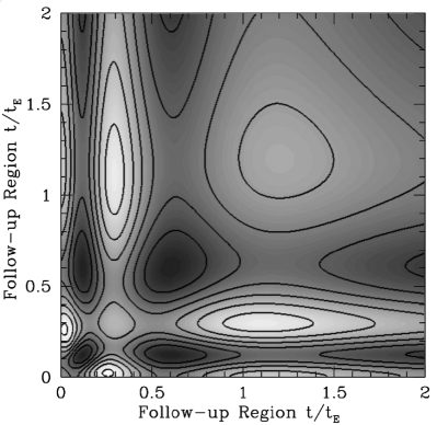
Figure 5: Number of additional uniformly distributed observations required for the same improvement as 8 focused observations (2 follow-up regions each with 4 observations). The seven contours are 2 (darkest regions), 4, 6, 8, 10, 12, & 14 (lightest regions). In this case $u_{min}=0.25$ and $f_{ll}=.25$. Values above (below) 8 indicate an advantage (disadvantage) relative to uniform follow-up.

In order to see the effect of adding multiple follow-up observations at two distinct times we compare this with adding evenly spaced observations. In Figure 5 we plot the increase (or decrease) in effectiveness of extra focused observations as a function of the two times at which they are taken. The contours around the light areas show regions of increased effectiveness, while dark areas show areas where the focused observations are less valuable than evenly spaced observations. In this example the effectiveness is increased by up to a factor two.

It is important to note that with more observations or higher accuracy in each follow-up region the advantage per added observation is reduced and the relative values of the various minimums vary, though they stay in roughly the same place. For practical use it is important to note that the time of the optimum second follow-up observation(s) varies with the time of the first follow-up observations(s). In practice one would need to calculate optimum observing times for an event in progress as a function of all the previous measurements.

One problem with the above approach is that without knowing the underlying parameters, particularly $t_{E}$, it is difficult to predict the best times to take follow-up data. To test if a practical experiment could be designed to take advantage of focused follow-up data we simulated an experiment. First we generated lightcurves with 80 points over $8t_{E}$ with .05 Gaussian errors at the baseline drawing $f_{ll}$ randomly from the interval $[.01,1)$ and $u_{min}$ randomly from the interval $(0,1)$ requiring $A_{max}^{\prime}>1.34$ in the HDE approximation. We also adjusted $t_{E}$ to keep $t_{E}^{\prime}\sim 10{\rm days}$ also using the HDE approximation. We then generated 9 follow-up observations over 3 days at the peak and fit the first half of the light curve plus the follow-up data. From this first fit we calculated the optimum times for two more bouts of follow-up. We generated these, both with 9 observations over 3 days, and then fit the entire lightcurve with the added 27 points. We also generated 27 points of follow-up uniformly distributed over the 20 days starting at the peak, added it to the initial lightcurve and fit the resulting data. To see the relative improvement for the two methods we calculate a parameter $\zeta=(f_{ll_{focused}}^{\prime}-f_{ll})/(f_{ll_{unfocused}}^{\prime}-f_{ll})$, which is the ratio of the error in blend fraction given by focused observations to the error in blend fraction given by uniform follow-up sampling. We plot the distribution of $\zeta$ in Figure 6 finding that our strategy gives an improvement $(\zeta<1)$ for 71% of the events and a worsening in 29% of the events. We find a substantial improvement ($\zeta<.5$) for 45% of the events, and and even larger improvement ($\zeta<0.1$) 18% of the time. Thus we conclude that for the the same amount of observing time we can make a more accurate measurement of $f_{ll}$ by focussing the follow-up observations.

Figure 6: The ratio $\zeta$ showing the advantage of a focused follow-up strategy for 71% of events ($\zeta<1$ - unshaded region). For 15% of the events in our simulation are outside the range of this plot $|\zeta|>2$.

In summary we find that observations concentrated at a few times can constrain the microlensing parameters as well as many measurements distributed throughout an event. The best place for these measurements are at the peak, in the falling/rising portion, and in the wings with regions between where added observations do no good. In most cases it is possible to constrain the event parameters well enough with the first half of the data and some follow-up observations near the peak to predict the last two optimum observing times.

5 Baseline Magnitude

The baseline magnitude of a lightcurve can in principle be very well determined since many measurements can be taken before or after the microlensing event. WP assumed that this was the case and so did not include the baseline magnitude as one of their fit parameters. In real microlensing surveys, however, it may be that the error in average magnitude is not entirely statistical, and may not average down as expected. There may be a systematic limit to the accuracy with which the baseline magnitude can be determined. In fact, detectors and telescope systems drift over time and so measurements made much later may actually reduce the accuracy of the baseline magnitude. To investigate the importance of the baseline magnitude, we created artificial lightcurves without any errors and fit them with a model with a fixed value of baseline magnitude that differed from the actual baseline magnitude by various amounts. Our results are shown in Figure 7. We find that the dependence on baseline is very strong for low amplification events and not as strong for higher amplifications events, but in any case even a 2% error in baseline magnitude determination can strongly bias the recovered blend fraction.

Figure 7: The recovered $f_{ll}$ for unblended light curves as a function of an input baseline magnitude (fixed at a given value). Forty points over 4 $t_{E}$ are used.

Next, to see how well baseline magnitudes converge in real data, we used the MACHO collaboration database of random stars (Alcock, et al. 2000). We looked at the $\chi^{2}/n_{dof}$ of a fit to a constant lightcurve for our real lightcurves and compared this to simulated ideal lightcurves with the same number of points and Gaussian errors. For the simulated Gaussian lightcurves we find the $\chi^{2}/n_{dof}$ distribution peaked near unity and distributed as expected, but for the real data the distribution of $\chi^{2}/n_{dof}$ is much broader. These two distributions are shown in Figure 8.

Figure 8: Actual distribution of $\chi^{2}/n_{dof}$ (top) for MACHO data and theoretical distribution of $\chi^{2}/n_{dof}$ (bottom)

As an estimate of the error in the baseline which arises due to the systematic drift and non-Gaussian nature of the magnitude errors, we calculated mean and median for the points in each of 146 lightcurves in MACHO field 119, one of the most frequently observed fields. We found that the distribution of mean minus median had a dispersion of 1.3% indicating that the error in the baseline flux is $\sim 1.3\%$. Referring to Figure 7 we see that for a typical event with $u_{min}=0.5$, this implies a typical spread in $f_{ll}$ of 0.18 due to baseline alone. Since half of all events have $u_{min}<0.5$, half of all events will have an even larger bias. For more sparsely sampled fields this dispersion due to error in baseline fit would be even larger.

6 Errors in Fit Parameters

From Macho Project data (Table 6 of Popowski et al. 2005) it seems blend fits return biased parameters. For the set of Macho clump giant events, which are believed to be minimally blended from their positions on the color magnitude diagram, many are best fit with blending. If the events are not blended then a systematic bias in the fits must make them appear to be blended. A systematic bias in recovered lensed-light fraction would lead to a bias in the optical depth as well. The MACHO collaboration investigated the blending of their clump giant sample and decided to use the parameters from the unblended fits. They also used a subsample of events that were less likely to be blended to check for a bias due to blending and found no such bias.

To test for a systematic bias we generate 1000 lightcurves with Gaussian errors for each of three different values for the error on each point: $\sigma=0.01$, $\sigma=0.05$, and $\sigma=0.15$. The recovered lensed-light fractions for these events are shown in Figure 9. As the error on individual datum increases the distribution of $f_{ll}^{\prime}$ becomes increasingly skewed. We find that while the mean $f_{ll}^{\prime}$ may not decrease, the most probable value does decrease. This reduction in the mode is at least partially compensated by the large tail of the distribution with $f_{ll}^{\prime}>1$, but for the small number of events a microlensing experiment observes it is unlikely that many of the few events with $f_{ll}^{\prime}\gg 1$ will be observed. Even if one event with $f_{ll}^{\prime}\gg 1$ is observed it may be ignored as it is an unphysical value of the parameter, thus leading to an underestimate of the average value of $f_{ll}$. Thus we find that as the errors in measurement increase blend fitting becomes more and more likely to return biased results. The direction of the bias is more often toward small values of $f_{ll}$. Thus events that are in reality unblended become more and more likely to return fit values implying that they are heavily blended.

Figure 9: Recovered $f_{ll}$ for data with Gaussian errors of $0.01,0.05,$ and $0.15$. As the errors on individual data points increase the distribution becomes increasingly skewed with the mode shifting toward 0 for larger errors. Also note that 11% of the $\sigma=0.05$ events and 24% of the $\sigma=0.15$ events had recovered $f_{ll}^{\prime}>2$ while none of the events with $\sigma=0.01$ were fit best with $f_{ll}^{\prime}>2$.

7 Conclusions

We find agreement with previous workers that blend fits are problematic, but can be useful especially for high magnification events. When performing blend fits it is helpful to get extra measurements near the peak and at other specific points along the lightcurve. We find that if care is not taken in the treatment of the lightcurve baseline magnitude the fit results can be severely biased and in real data the errors returned on fit parameters should be treated with caution. We find that blend fits return a biased, skewed distribution of the underlying parameters tending to indicate more blending than actually exists. Finally, note that when the microlensing event contains signal from other physical effects such as weak parallax or binary effects blend fits can yield unreliable results. These effects are not rare, and since the difference between blended and unblended lightcurves is small, even an almost undetectable real deviation from the standard point-source-point-lens lightcurve can render blend fit results meaningless.

References

- (1) Afonso, C., et al. 2003, A&A, 404, 145
- (2) Alard, C., Mao, S., & Guibert, J., 1995, A&A, 300, L17
- (3) Alard, C. 1997, A&A, 321, 424
- (4) Alcock, C., et al., 1993, Nature, 365, 621
- (5) Alcock, C., et al., 1997a, ApJ, 486, 697
- (6) Alcock, C., et al., 1997b, ApJ, 479, 119
- (7) Alcock, C., et al., 2000, ApJ, 542, 281
- (8) Alcock, C., et al., 2001, ApJ, 552, 582
- (9) Aubourg, E. et al., 1993, Nature, 365, 623
- (10) CERN Lib., 2003, http://wwwasdoc.web.cern.ch /wwwasdoc/minuit/minmain.html
- (11) de Jong, J.T.A. et al., 2004, A&A, 417, 461
- (12) DiStefano, R. & Esin, A.A., 1995, ApJL 448, L1
- (13) Han, C., 1999, MNRAS, 309, 373
- (14) Han, C., & Gould, A., 2003, ApJ, 592, 172
- (15) Gould, A., 2003, astro-ph/0310577
- (16) Gould, A. & An, J.H., 2002, ApJ, 565, 1381
- (17) Griest, K., et al., 1991, ApJ, 372, L79
- (18) Lasserre, T., et al., 2000, AA, 355, L39
- (19) Paczyński , B., 1991, ApJ, 371, L63
- (20) Paulin-Henriksson, S., et al., 2003, A&A, 405, 15
- (21) Popowski, P., et al., 2005, To appear in ApJ, astro-ph/0410319
- (22) Sumi, T., et al. 2005, astro-ph/0502363
- (23) Thomas, C.L., et al. 2005, To appear in ApJ, astro-ph/0410319
- (24) Udalski, A., et al. 1994, ApJ, 426, L69
- (25) Woźniak , P. & Paczyński , B., 1997, ApJ, 487, 55
- (26)