Optical Depths and Time-Scale Distributions in Galactic Microlensing

Abstract

We present microlensing calculations for a Galactic model based on Han & Gould (2003), which is empirically normalised by star counts. We find good agreement between this model and data recently published by the MACHO and OGLE collaborations for the optical depth in various Galactic fields, and the trends thereof with Galactic longitude $l$ and latitude $b$. We produce maps of optical depth and, by adopting simple kinematic models, of average event time-scales for microlensing towards the Galactic bulge. We also find that our model predictions are in reasonable agreement with the OGLE data for the expected time-scale distribution. We show that the fractions of events with very long and short time-scales due to a lens of mass $M$ are weighted by $M^{2}\,n(M)\,{\rm d}M$ and $M^{-1}\,n(M)\,{\rm d}M$ respectively, independent of the density and kinematics of the lenses.

1 Introduction

A microlensing event occurs when a luminous object is temporarily magnified by a massive body, such as a star or dark matter object, passing close to the line of sight and acting as a gravitational lens. Paczyński (1986) advocated searching for microlensing events towards the Large Magellanic Cloud in order to detect dark matter in the Galactic halo. Soon three separate collaborations were conducting systematic searches: OGLE (Udalski et al., 1992), EROS (Aubourg et al., 1993), and MACHO (Alcock et al., 1993), between them observing the Large and Small Magellanic Clouds and the Galactic bulge. Other groups such as MOA (e.g. Bond et al. 2001) have since joined the search, and thousands of microlensing events have now been detected (e.g., Alcock et al. 2000; Wozniak et al. 2001; Sumi 2003), almost all towards the bulge. A much smaller number of microlensing candidates have also been identified toward the Large Magellanic Cloud (e.g., Alcock et al. 2000) and M31 (e.g., Novati et al. 2005). One of the main aims of all these observations is to accurately measure the optical depth, $\tau$ – the probability of seeing a microlensing event at any given instant – which can provide much information about the structure and mass distribution of the Galaxy and its halo.

Since the first estimates of $\tau$ by Paczyński (1991) and Griest (1991), predictions based on increasingly refined models have consistently and significantly disagreed with measurements based on increasingly large sets of observational data. However, there are now signs of convergence. Han & Gould (2003) – hereafter HG03 – used star counts from the Hubble Space Telescope (HST) to normalise their Galactic model, predicting $\tau=1.63\times 10^{-6}$ towards Baade’s window (BW), based on lensing of red clump giants (RCGs). They noted reasonable agreement with two recent measurements towards the bulge, also based on RCGs, of $\tau=2.0\,(2.13)\pm 0.4\times 10^{-6}$ and $\tau=0.94\,(1.08)\pm 0.30\times 10^{-6}$, from the MACHO (Popowski et al., 2001) and EROS (Afonso et al., 2003) collaborations, respectively. The numbers in parentheses are from table 2 of Afonso et al. (2003), who enabled a better comparison between all bulge optical depth measurements to be made by adjusting the values for their offset from BW. Now from 7 years of MACHO survey data, Popowski et al. (2004) report $\tau=2.17^{+0.47}_{-0.38}\times 10^{-6}$ at $(l,b)=(1.50^{\circ},-2.68^{\circ})$, which is in excellent agreement with recent theoretical predictions, including the Han & Gould result. Most recently, from the OGLE-II survey Sumi et al. (2005) find $\tau=2.37^{+0.53}_{-0.43}\times 10^{-6}$ at $(l,b)=(1.16^{\circ},-2.75^{\circ})$, which is also consistent with the latest MACHO survey value.

In this paper we generate Monte Carlo simulations of the Galaxy based on HG03. The outline of the paper is as follows. §2 describes the model and theory, and §3 presents our results: In §3.1 we reproduce the HG03 $\tau_{\rm BW}$, and then compare our predicted $\tau$ with the recent MACHO and OGLE results in various directions. §3.2 presents maps of optical depth and average event time-scale (duration). These maps can be compared with observations in any direction. In §3.3 we predict the event rate as a function of time-scale and compare this to the distribution observed by OGLE. In §3.4 we show how at both long and short times the time-scale distribution is directly related to the lens mass function. We summarise our results in §4.

2 The Model

2.1 Bulge and disc mass models

Dwek et al. (1995) compared various hypothetical mass density models of the bulge to the infrared light density profile seen by the Cosmic Background Explorer (COBE) satellite. We use the G2 (barred) model from their table 1, with $R_{\rm max}$ = 5 kpc. The bar is inclined by $13.4^{\circ}$ to the Galactic centre line of sight, and the distance to the Galactic centre is set at 8 kpc. Dwek et al. used 8.5 kpc, so we adjust their model parameters accordingly. The model is then normalised by HST star counts (see the end of §2.2). This independent constraint can be used to normalise any bulge model.

For the disc, we use the local disc density model of Zheng et al. (2001), as extended to the whole disc by HG03. As the disc model is relatively secure (HG03), it will contribute only small uncertainties to predictions of the optical depth, so it is not renormalised as for the bulge model.

2.2 Source and lens populations

The optical depths reported by Popowski et al. (2004) are based on lensing of RCGs in the bulge, and HG03 assume only bulge RCG sources in their model. Sumi et al. (2005) observed lensing of red giants and red super giants as well as RCGs. We assume that these different types of stars follow the same bar density distribution and are bright enough to be seen throughout the bar, which corresponds to the case with $\gamma=0$ in the following eq. (5).

Our lens mass function is generated as in HG03. Their unnormalised bulge mass function assumes initial star formation according to

$${\rm d}N/{\rm d}M=k(M/M_{\rm brk})^{\alpha},$$ (1)

where $M_{\rm brk}=0.7\ \rm M_{\odot}$, $\alpha=-2.0$ for $M>M_{\rm brk}$, and $\alpha=-1.3$ for $M\leq M_{\rm brk}$, consistent with observations by Zoccali et al. (2000). However HG03 extended this beyond the latter’s lower limit of $M\sim 0.15\ \rm M_{\odot}$ to a brown dwarf cut-off of $M\sim 0.03\ \rm M_{\odot}$. We assume objects with masses 0.03–0.08 $\rm M_{\odot}$ and 0.08–1 $\rm M_{\odot}$ become brown dwarfs (BD) and main-sequence stars (MS) respectively, 1–8 $\rm M_{\odot}$ stars evolve into 0.6 $\rm M_{\odot}$ white dwarfs (WD), 8–40 $\rm M_{\odot}$ stars become 1.35 $\rm M_{\odot}$ neutron stars (NS), and anything more massive forms a 5 $\rm M_{\odot}$ black hole (BH).

For MS stars we use the mass-luminosity relation of Cox (1999), and take all other lenses to be dark. The model is then normalised by comparing extinction-adjusted MS counts to HST star counts (Holtzman et al., 1998) as described in HG03. The same mass function and luminosity relation are also used for the disc. Strictly they should be independently estimated, but any uncertainties are small compared to others involved as we find disc stars account for only $\sim 20$ per cent of the total number of stars in BW.

2.3 Kinematic model

To calculate the event rate, we must also specify the velocities of the lenses, sources and observer. The observer velocity $v_{\rm O}$ is assumed to follow the Galactic rotation, so the two velocity components in $l$ and $b$ are given by

$$v_{\rm O,l}=v_{\rm O,{\rm rot}}=220{\rm\ kms}^{-1},\ \ \ \ \ \ v_{\rm O,b}=0.$$ (2)

The lens and source velocities in the $l$ and $b$ directions are given by

$$v_{\rm l}=v_{\rm rot}+v_{\rm rand,l},\ \ \ \ \ \ v_{\rm b}=v_{\rm rand,b},$$ (3)

where the rotation velocity $v_{\rm rot}$ and the random velocity $v_{\rm rand}$ are from Han & Gould (1995): for the disc $v_{\rm rot}=220{\rm\ kms}^{-1}$, and for the bar $v_{\rm rot}$ is given by projecting $v_{\rm max}=100{\rm\ kms}^{-1}$ across the line of sight according to

$$v_{\rm rot} = v_{\rm max}\left(x\over 1\ {\rm kpc}\right)\ \ \ \ \ \ (R<1\ {\rm kpc},\ {\rm solid\ body\ rotation}),$$

$$v_{\rm rot} = v_{\rm max}\left(x\over R\right)\ \ \ \ \ \ \ \ \ \ \ (R\geq 1\ {\rm kpc},\ {\rm flat\ rotation}),$$ (4)

where $R=(x^{2}+y^{2})^{1/2}$, and the coordinates $(x,y,z)$ have their origin at the Galactic centre, with the $x$ and $z$ axes pointing towards the Earth and the North Galactic Pole respectively. The random velocity components $v_{\rm rand,l}$ and $v_{\rm rand,b}$ are assumed to have Gaussian distributions. For the disc $\sigma_{\rm l,\,b}=(30,\,20){\rm\ kms}^{-1}$, and for the bar we use $\sigma_{\rm x,\,y,\,z}$ = (110, 82.5, 66.3)${\rm\ kms}^{-1}$ as found by Han & Gould (1995) using the tensor virial theorem (see also Sumi, Eyer & Woźniak 2003, and Kuijken & Rich 2002). These values should be altered slightly as HG03 used a different normalisation. This may affect our results slightly, but it is re-assuring that our results based on such a simple kinematic model appear to agree with the data quite well (see §3).

2.4 Optical depth and event rate

$\tau$ in any given direction is an average over the optical depths of all the source stars in that direction. The optical depth to a particular star is defined as the probability that it is within the Einstein radius (see below) of any foreground lenses. Hence more distant stars, although fainter and less likely to be detected, have higher optical depths (Stanek, 1995). HG03 accounted for this with the term $\gamma$ in the calculation of observed optical depth:

$$\langle\tau\rangle_{\gamma}={4\pi G\over c^{2}}{\int_{0}^{\infty}{\rm d}D_{\rm s}D_{\rm s}^{2-\gamma}\rho(D_{\rm s})\int_{0}^{D_{\rm s}}{\rm d}D_{\rm d}\rho(D_{\rm d})D_{\rm d}(D_{\rm s}-D_{\rm d})/D_{\rm s}\over\int_{0}^{\infty}{\rm d}D_{\rm s}D_{\rm s}^{2-\gamma}\rho(D_{\rm s})},$$ (5)

where $D_{\rm s}$ and $D_{\rm d}$ are the distances to the source and deflector (lens), and $\rho(D_{\rm s})$ and $\rho(D_{\rm d})$ are the source number density and lens mass density. RCGs and other bright stars in the bulge can be identified independently of their distance, so $\gamma=0$. Eq. (5) was originally presented (in a slightly different form) by Kiraga & Paczyński (1994), who also derived an expression for the lensing event rate $\Gamma$. We give this here in terms of $\gamma$, and account for variation in lens mass by bringing the term $M^{-1/2}$ inside the integral:

$$\Gamma = {4G^{1/2}\over c}\int_{0}^{\infty}{\rm d}D_{\rm s}D_{\rm s}^{2-\gamma}\rho(D_{\rm s})$$ (6)

$$\times{\int_{0}^{D_{\rm s}}{\rm d}D_{\rm d}\rho(D_{\rm d})v[D_{\rm d}(D_{\rm s}-D_{\rm d})/MD_{\rm s}]^{1/2}\over\int_{0}^{\infty}{\rm d}D_{\rm s}D_{\rm s}^{2-\gamma}\rho(D_{\rm s})},$$

where $v$ is the lens-source relative transverse velocity,

$$v=({v_{\rm l}}^{2}+{v_{\rm b}}^{2})^{1/2},$$ (7)

and its components in the Galactic $l$ and $b$ coordinates, $v_{\rm l}$ and $v_{\rm b}$, are related to the observer, lens and source velocities by

$$v_{\rm l,b}=\left((v_{\rm D}-v_{\rm O})+(v_{\rm O}-v_{\rm S}){D_{\rm d}\over D_{\rm s}}\right)_{\rm l,b},$$ (8)

where $v_{\rm D}$ and $v_{\rm S}$ are the deflector (lens) and source transverse velocities; their components in the $l$ and $b$ directions are given in eq. (3).

The time-scale of an event $t_{\rm E}$ is defined as the time taken for a source to cross the Einstein radius of the lens $r_{E}$ (Paczyński, 1996):

$$t_{\rm E}={r_{E}\over v}\ \ \ \ \ \ \ \ r_{E}=\left({4GM\over c^{2}}{D_{\rm d}(D_{\rm s}-D_{\rm d})\over D_{\rm s}}\right)^{1/2}.$$ (9)

3 Results

3.1 Optical depth in MACHO and OGLE fields

HG03 calculated $\tau=(0.98,0.65,1.63)\times 10^{-6}$ towards BW for bulge, disc, and all lenses respectively. Our equivalent values are (1.06, 0.65, 1.71) $\times 10^{-6}$. HG03 noted that the value of $\gamma$ makes little difference to $\tau$ for disc lenses, but for bulge lenses $\tau$ becomes $0.86\times 10^{-6}$ when $\gamma=1$. We find $\tau=0.92\times 10^{-6}$ in this case. Our results for bulge lenses differ by 7–8 per cent from HG03’s due to a slight difference in implementation of the bulge model normalisation. We find that allowing MS disc lenses to also act as sources themselves makes a negligible difference to the total value of $\tau$.

The MACHO measurement (Popowski et al., 2004) of $\tau=2.17^{+0.47}_{-0.38}\times 10^{-6}$ at $(l,b)=(1.50^{\circ},-2.68^{\circ})$, was obtained from a sub-sample of their observed fields, the ‘Central Galactic Region’ (CGR), which covers 4.5 deg² and contains 42 of the 62 RCG microlensing events seen. The coordinates $(1.50^{\circ},-2.68^{\circ})$ are a weighted average position of these fields; the unweighted average is $(l,b)=(1.55^{\circ},-2.82^{\circ})$. Optical depths were also given for a region ‘CGR+3’ that contains 3 additional fields, and for all 62 events. In Table 1 we compare our expected values to each of these results, and to $\tau$ reported for each of the individual CGR fields.

OGLE’s measurement (Sumi et al., 2005) of $\tau=2.37^{+0.53}_{-0.43}\times 10^{-6}$ at $(l,b)=(1.16^{\circ},-2.75^{\circ})$ made use of 32 RCG events, in 20 of their 49 fields, where $(l,b)=(1.16^{\circ},-2.75^{\circ})$ is the weighted average field position. $\tau$ was also given for each field; we compare our values to all of these results in Table 2.

Note that any significant disagreement occurs only in individual fields, and that in only 1 of the 6 fields (MACHO and OGLE) with $>4$ events (OGLE #30) does our value lie far outside the stated $1\sigma$ uncertainty.

Table 3 shows the percentage contributions to the total optical depth and event rate from the different types of lenses. The disc lenses contribute about 37 per cent of the optical depth and a slightly smaller fraction (31 per cent) of the event rate. We see that 62 per cent of all events have luminous (MS) lenses, the other 38 per cent are dark (BD, WD, NS and BH). The NSs and BHs contribute about 9 per cent of the optical depth but only 4 per cent of the event rate. This is because the events caused by stellar remnants on average have longer time-scales, and thus they occur less frequently.

Region/field	${N_{\rm events}}^{*}$	($l$, $b$) (∘)	$\tau_{\rm MACHO}(\times 10^{-6})$	$\tau_{\rm model}(\times 10^{-6})$
CGR†	42	(1.50, -2.68)	$2.17^{+0.47}_{-0.38}$	2.43
CGR‡	42	(1.55, -2.82)	–	2.33
CGR+3	53	(1.84, -2.73)	$2.37^{+0.47}_{-0.39}$	2.34
All events	62	(3.18, -4.30)	$1.21^{+0.21}_{-0.21}$	1.32
108	6	(2.30, -2.65)	$2.04\pm 0.92$	2.31
109	2	(2.45, -3.20)	$0.58\pm 0.41$	1.96
113	3	(1.63, -2.78)	$0.55\pm 0.35$	2.34
114	3	(1.81, -3.50)	$1.19\pm 0.74$	1.87
118	7	(0.83, -3.07)	$2.85\pm 1.35$	2.25
119	0	(1.07, -3.83)	–	1.74
401	7	(2.02, -1.93)	$5.13\pm 2.16$	2.85
402	10	(1.27, -2.09)	$3.95\pm 1.50$	2.89
403	4	(0.55, -2.32)	$1.16\pm 0.66$	2.83

Table 1: Comparison of model and MACHO optical depths for the Central Galactic Region (CGR) and individual fields. ^∗Number of events seen by MACHO. ^†Weighted average ($l$, $b$). ^‡Unweighted average ($l$, $b$).

Region/field	${N_{\rm events}}^{*}$	($l$, $b$) (∘)	$\tau_{\rm OGLE}(\times 10^{-6})$	$\tau_{\rm model}(\times 10^{-6})$
All fields†	32	(1.16, -2.75)	$2.37^{+0.53}_{-0.43}$	2.43
1	0	(1.08, -3.62)	–	1.87
2	1	(2.23, -3.46)	$2.31\pm 2.31$	1.85
3	4	(0.11, -1.93)	$3.99\pm 2.07$	3.20
4	5	(0.43, -2.01)	$2.93\pm 1.39$	3.09
20	1	(1.68, -2.47)	$1.15\pm 1.15$	2.54
21	0	(1.80, -2.66)	–	2.39
22	1	(-0.26, -2.95)	$0.79\pm 0.79$	2.42
23	0	(-0.50, -3.36)	–	2.13
30	6	(1.94, -2.84)	$8.88\pm 3.89$	2.26
31	1	(2.23, -2.94)	$2.10\pm 2.10$	2.15
32	1	(2.34, -3.14)	$0.87\pm 0.87$	2.02
33	2	(2.35, -3.66)	$9.69\pm 7.38$	1.73
34	2	(1.35, -2.40)	$3.80\pm 2.69$	2.65
35	2	(3.05, -3.00)	$2.99\pm 2.19$	1.98
36	0	(3.16, -3.20)	–	1.85
37	2	(0.00, -1.74)	$2.06\pm 1.65$	3.39
38	2	(0.97, -3.42)	$2.68\pm 2.09$	2.01
39	3	(0.53, -2.21)	$1.51\pm 0.90$	2.92
45	0	(0.98, -3.94)	–	1.68
46	0	(1.09, -4.14)	–	1.56

Table 2: Comparison of model and OGLE optical depths. ^∗Number of events seen by OGLE. ^†Weighted average ($l$, $b$).

	Location/type of lens
	Bar	Disc	BD	MS	WD	NS	BH
Optical depth	63	37	7	62	22	6	3
Event rate	69	31	17	62	17	3	1

Table 3: Percentage contributions, to the total predicted $\tau$ and $\Gamma$, from different types of lens.

Figure 1: Average optical depth in latitude (left panel) and longitude (right panel) strips, for $-5.5^{\circ}\leq b\leq 5.5^{\circ}$ and $-5.5^{\circ}\leq l\leq 5.5^{\circ}$ respectively. The solid line shows the model prediction, while the open and solid circles are data points from MACHO (fig. 14, Popowski et al. 2004) and OGLE (fig. 12, Sumi et al. 2005) respectively.

In their figs. 12 and 14 respectively, Sumi et al. (2005) and Popowski et al. (2004) plot average optical depths in latitude and longitude strips. We produce similar plots in Fig. 1, with the OGLE and MACHO data points shown. In both sets of strips the model is in good agreement with both sets of data. The single data point at negative $l$ is based on only one microlensing event, so the discrepancy has low statistical significance.

3.2 Maps of optical depth and average event time-scale

Figs. 2 and 3 are maps of expected optical depth and average event time-scale. We can clearly see higher optical depths and longer time-scales at negative galactic longitude. This is due to the inclination of the bar to the line of sight. At positive longitude the bar is closer to us, and the line of sight cuts through the bar at a steeper angle. Hence there are fewer potential lenses, in either the disc or the bar, between us and any bar source, and so $\tau$ is smaller. Also, objects rotating around the Galactic centre have a smaller component of their velocity along the line of sight, so average transverse velocities will be greater, and average time-scales shorter. At negative longitude, the line of sight passes through more of the disc and cuts the bar at a shallower angle. Hence we see higher optical depths and smaller transverse velocities, and thus longer average time-scales.

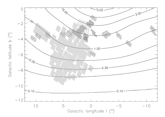
Figure 2: Map of expected optical depth. The MACHO and OGLE fields are shown by the large and small grey boxes, respectively. For the MACHO fields, the crosshatch pattern indicates the CGR subset listed in Table 1. For OGLE, the crosshatch pattern denotes those fields not listed in Table 2. The small square indicates BW. Contour levels are at $(0.1,0.2,0.3,0.5,1,2,3,4,5)\times 10^{-6}$.

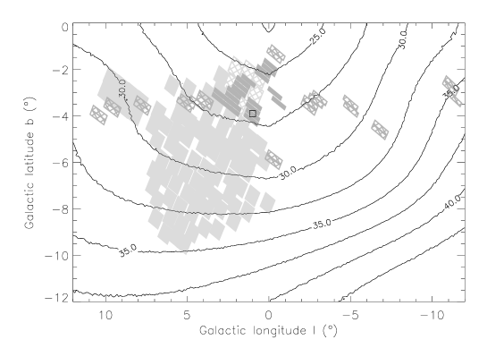
Figure 3: Map of expected average event time-scale. The MACHO and OGLE fields are shown by the large and small grey boxes, respectively. For the MACHO fields, the crosshatch pattern indicates the CGR subset listed in Table 1. For OGLE, the crosshatch pattern denotes those fields not listed in Table 2. The small square indicates BW. Contour levels are at 22.5, 25, 27.5, 30, 32.5, 35, 37.5, 40 and 42.5 d.

Figure 4: $\tau$ as a function of $b$, for $l$ = $3.9^{\circ}$. Our model slope is almost identical for bar angles of $13.4^{\circ}$ and $20^{\circ}$. The profile of Bissantz & Gerhard (2002) diverges from ours at $b\approx-3^{\circ}$, increasing rapidly towards the mid-plane ($b=0^{\circ}$).

We wish to compare our maps to others. Evans & Belokurov (2002) produced red clump optical depth maps for three Galactic models, but while two of these appear similar to ours, they do not agree. One of those models was also used to make a time-scale map, which is quite different to ours. This is not surprising since, as well as using a different mass model, their mass function, velocities and velocity dispersions were also different. (In fact their timescale map has two sets of contours, to show the effects of including and excluding bar streaming. Without streaming their mean timescales are much shorter than ours, and with it they are greater by a factor $\sim 3$, much longer than ours. Such a large variation is puzzling, and we are cautious about comparing their map to ours).

In their fig. 16, Bissantz & Gerhard (2002) presented an optical depth map for RCG sources, with a bar angle of $20^{\circ}$. For $b$ $\la-3^{\circ}$ it appears quite similar to ours, but moving towards the Galactic centre $\tau$ climbs far more steeply than in our map. This is best seen by comparison to their fig. 17, where they plot $\tau$ as a function of $b$, for $l$ = $3.9^{\circ}$. This is shown in Fig. 4 with equivalent profiles for our model. We see how rapidly Bissantz & Gerhard’s profile diverges from ours towards $b=0^{\circ}$. We also see that changing the bar angle in our model from $13.4^{\circ}$ to $20^{\circ}$ does not explain this difference. Instead it is probably due to the density in their bulge mass model increasing much faster towards the mid-plane. The observational data for the mid-plane are limited due to heavy extinction, and so mass models are not well-constrained in this region. Given the difficulty in obtaining any measurement of $\tau$ at small latitude, it is difficult at present to test either profile there.

3.3 Time-scale distributions

Fig. 5 shows the event rate as a function of time-scale towards the OGLE coordinates $(l,b)=(1.16^{\circ},-2.75^{\circ})$, for bar (thin line), disc (dashed line) and all (bold line) lenses. There is good agreement with the asymptotic power-law tails $d\Gamma/d({\rm log}\ t_{\rm E})\propto$ ${t_{\rm E}}^{3}$, ${t_{\rm E}}^{-3}$ for very short and long time-scales, respectively (Mao & Paczyński, 1996). The disc lensing events have an average time-scale of 26.3 d, slightly longer than the bulge lensing events’ average of 25.7 d, as also found by Kiraga & Paczyński (1994). The average time-scale for all events is 25.9 d.

Figure 5: Predicted microlensing event rate as a function of time-scale, towards $(l,b)=(1.16^{\circ},-2.75^{\circ})$. The bold line represents all lenses. The thin and dashed lines represent the bar and disc lenses, respectively. The two dotted lines are asymptotic tails $d\Gamma/d({\rm log}\ t_{\rm E})\propto$ ${t_{\rm E}}^{3}$, ${t_{\rm E}}^{-3}$ for very short and long time-scales, respectively.

Figure 6: Microlensing event rate as a function of time-scale, towards $(l,b)=(1.16^{\circ},-2.75^{\circ})$. The solid line shows the model prediction, and the OGLE observed distribution (corrected for detection efficiency) is shown as a histogram.

In Fig. 6 we renormalise our time-scale distribution (for all lenses) and compare it to that seen by OGLE, as corrected for detection efficiency (see fig. 14 in Sumi et al. 2005). We do not compare to the time-scale distribution seen by Popowski et al. (2004) – they assumed that the effect of blending on RCG sources is negligible, but Sumi et al. (2005) found $\approx$ 38 per cent of OGLE-II events with apparent RCG sources were really due to faint stars blended with a bright companion. Fortunately, they also showed that blending has little effect on estimates of $\tau$ due to partial cancellation of its different effects, a point also made by Popowski et al. (2004). However, time-scale distributions will be significantly shifted towards shorter events. As a result, the MACHO time-scale distribution (not shown) has a significant excess at short time-scales compared with our model.

Our time-scale distribution shows reasonable agreement with OGLE’s. The Kolmogorov–Smirnov (KS) test shows that the predicted and observed distributions are consistent at a $\approx 52$ per cent confidence level. Our average time-scale of 25.9 d is in excellent agreement with OGLE’s corrected average of $28.1\pm 4.3$ d. Our median and quartiles are (19.2, 11.2, 31.7) d, respectively.

The event time-scale distribution from the data still has large uncertainties due to the limited number of events. It is apparent that the data have not yet reached the predicted asympototic behaviour at short and long time scales, so a more stringent test on the model is not yet possible.

Bissantz, Debattista & Gerhard (2004, see also ) have also modelled the time-scale distribution. They reproduced that from MACHO’s 99 DIA events (Alcock et al., 2000) centred at $(l,b)=(2.68^{\circ},-3.35^{\circ})$. However, both distributions are clearly shifted towards short time-scales compared to our model prediction in the same direction (this is not shown, as it is very close to the solid line in Fig. 6). Although the DIA method is less prone to the systematics of blending (Sumi et al., 2005), it is still possible that the MACHO DIA time-scale distribution is somewhat affected. The most important difference between our model and Bissantz et al.’s is that in order to match the data at short time-scales, they adopted a Schecter mass function, $n(M)\propto M^{-2.35}$ for $M\leq 0.35\ \rm M_{\odot}$ down to 0.04 $\rm M_{\odot}$, steeper than our mass function, $n(M)\propto M^{-1.3}$ for $M<0.7\ \rm M_{\odot}$. As a result, their median lens mass is much smaller than ours (0.11 $\rm M_{\odot}$ vs. 0.35 $\rm M_{\odot}$, weighted by event rate). The different kinematics may also have a noticeable effect on the timescales, but their more realistic dynamical model does not allow a simple comparison to be made.

3.4 Fractional contributions to event rate – mass weightings

Fig. 7 shows the fractional contributions to the total event rate, as a function of event time-scale, for the different types of lens (BD, MS, WD, NS and BH) as indicated. At short time-scales ($t_{\rm E}\la 4$ d), the brown dwarfs dominate the event rate, while at long time-scales ($t_{\rm E}\ga 100$ d), the stellar remnants become increasingly important. There is asymptotic behaviour at both long and short time-scales. We find that the fractional contribution from a lens of mass $M$ is weighted by $M^{2}\,n(M)\,{\rm d}M$ and $M^{-1}\,n(M)\,{\rm d}M$, respectively. In the Appendix we derive these weightings from eq. (6). (The scaling at long event tails has already been derived by Agol et al. 2002). Table 4 shows that direct calculation of these asymptotic fractions from the mass function gives results that clearly agree with the trends in Fig. 7. These weightings are independent of the density and kinematics of the lens population, and hence provide valuable information about the lens mass function.

Time-scale	BD	MS	WD	NS	BH
Long	0.53	44	20	12	24
Short	72	27	1.5	0.078	0.0032

Table 4: Percentage contributions to the total predicted event rate, at long and short time-scales, from the different types of lens.

Figure 7: Fractional contributions to total expected event rate, as a function of event time-scale, from BD, MS, WD, NS and BH lenses as indicated. The solid and dashed lines represent the bar and disc lenses, respectively. The asymptotic fractions at long and short time-scales are a function of the lens mass only (see text).

4 Summary

In this paper, we have used a simple Galaxy model normalised by star counts (Han & Gould, 2003) to predict the microlensing optical depth. Combined with simple kinematic models, we also predict maps and distributions of the time-scale distributions. We have shown that the fraction of long and short events contributed by a lens of mass $M$ is weighted by $M^{2}\,n(M)\,{\rm d}M$ and $M^{-1}\,n(M)\,{\rm d}M$ respectively. If the tails of this distribution can be accurately determined from observations, we have a direct probe of the lens mass function.

It is remarkable that this emprically-normalised model based on the COBE G2 model (Dwek et al., 1995) shows good agreement with data recently published by the MACHO and OGLE collaborations (Sumi et al. 2005 and Popowski et al. 2004) for the optical depth in various Galactic fields, and its trends with $l$ and $b$. Our maps of optical depth and average event time-scale cover a large area of the sky, and can be compared to future determinations of $\tau$ in similar areas when they become available. The expected distribution of the event time-scale also appears to show good agreement with the recently published OGLE data (Sumi et al., 2005). However, the numbers of microlensing events used (42 and 32) in the recent MACHO and OGLE analyses are still small, so the test on the models is not yet stringent. When the much larger database of microlensing events ($\sim$ thousands) is analysed, then a full comparison with the models will become much more discriminating.

Appendix A Event rate weightings at long and short time-scales

As described in §3.4, the microlensing event rate shows asymptotic behaviour at both long and short time-scales. We show here that this is directly related to the lens mass function, specifically, the fractional contributions are weighted by $M^{2}\,n(M)\,{\rm d}M$ and $M^{-1}\,n(M)\,{\rm d}M$, at very long and short time-scales respectively.

The event rate is given by eq. (6). However, as the mass dependence of the asympototic behaviour is the same for sources at different distances, we shall ignore the source distance dependences here. Therefore for a source at distance $D_{\rm s}$ and a population of lenses each with identical velocity $v$ and mass $M$, the event rate is given by

$$\Gamma={4G^{1/2}\over c}\int_{0}^{D_{\rm s}}\rho(D_{\rm d})\,v\left({D_{\rm d}(D_{\rm s}-D_{\rm d})\over MD_{\rm s}}\right)^{1/2}{\rm d}D_{\rm d},$$ (10)

where $\rho(D_{\rm d})$ is the lens mass density at $D_{\rm d}$.

In reality, $v$ and $M$ both vary. The velocity probability distribution, ${\rm p}(v)\,{\rm d}v$, can usually be approximated by a two-dimensional Maxwellian distribution

$${\rm p}(v)\,{\rm d}v={1\over\sigma^{2}}\exp(-v^{2}/2\sigma^{2})\,v\,{\rm d}v,$$ (11)

where $\sigma$ is the velocity dispersion. For constant $M$, the factor $\rho(D_{\rm d})$ in eq. (10) is simply the total mass density. When $M$ varies, the event rate depends on the lens mass function, i.e. on how the total mass is partitioned into lenses of different masses. We assume that this is the same everywhere. The mass density for lenses with $M\rightarrow M+\,{\rm d}M$ can be written as a product of ${\rm f}(D_{\rm d})\,n(M)\,{\rm d}M$, where ${\rm f}(D_{\rm d})$ indicates the distance dependence and $n(M){\rm d}M$ is the number density of lenses between $M\rightarrow M+\,{\rm d}M$.

Integrating over the mass and velocity distributions and using the fact that $\rho(M){\rm d}M=M{\rm f}(D_{\rm d})\,n(M)\,{\rm d}M$, we obtain

$$\Gamma=2A^{1/2}\int_{0}^{D_{\rm s}}{D_{\rm eff}}^{1/2}{\rm f}(D_{\rm d})\,{\rm d}D_{\rm d}\int n(M)M^{1/2}\,{\rm d}M\int v\,{\rm p}(v)\,{\rm d}v,$$ (12)

where $A={4G/c^{2}}{\rm\ and\ }D_{\rm eff}=D_{\rm d}(D_{\rm s}-D_{\rm d})/D_{\rm s}$. We can now rewrite the time-scale equation (eq. 9)

$$t_{\rm E}={r_{E}\over v} = \left({4GM\over c^{2}}{D_{\rm d}(D_{\rm s}-D_{\rm d})\over D_{\rm s}}\right)^{1/2}v^{-1}$$ (13)

$$= {A^{1/2}M^{1/2}{D_{\rm eff}}^{1/2}\over v},$$

The typical transverse velocity is $\sim\sigma$, and this defines a characteristic time-scale as

$$t_{\sigma}={A^{1/2}M^{1/2}{D_{\rm eff}}^{1/2}\over\sigma}.$$ (14)

The short and long tails satisfy $t_{\rm E}\ll t_{\sigma}$ and $t_{\rm E}\gg t_{\sigma}$, respectively.

A.1 Behaviour at long time-scales

As can be seen from eq. (13), the long time-scale events occur when the lens and source both move approximately parallel to each other and perpendicular to the line of sight. In this case, the transverse velocity is close to zero ($v\ll\sigma$) and the time-scale becomes long.

For events with time-scales longer than $t_{\rm long}(\gg t_{\sigma})$, the transverse velocity must satisfy

$$v<{A^{1/2}M^{1/2}{D_{\rm eff}}^{1/2}\over t_{\rm long}}\ll\sigma.$$ (15)

The exponential factor $\exp(-v^{2}/2\sigma^{2})$ approaches unity, and so we have

$$\Gamma(>t_{\rm long}) = {2A^{1/2}\over\sigma^{2}}\int_{0}^{D_{\rm s}}{D_{\rm eff}}^{1/2}{\rm f}(D_{\rm d})\,{\rm d}D_{\rm d}\int n(M)M^{1/2}\,{\rm d}M\int_{0}^{A^{1/2}M^{1/2}{D_{\rm eff}}^{1/2}\over t_{\rm long}}v^{2}{\rm d}v$$ (16)

$$= {2A^{1/2}\over\sigma^{2}}\int_{0}^{D_{\rm s}}{D_{\rm eff}}^{1/2}{\rm f}(D_{\rm d})\,{\rm d}D_{\rm d}\int n(M)M^{1/2}\,{\rm d}M\times{1\over 3}\left({A^{3/2}M^{3/2}{D_{\rm eff}}^{3/2}\over{t_{\rm long}}^{3}}\right)$$

$$= {2A^{2}\over 3\sigma^{2}{t_{\rm long}}^{3}}\int_{0}^{D_{\rm s}}{D_{\rm eff}}^{2}{\rm f}(D_{\rm d})\,{\rm d}D_{\rm d}\int n(M)M^{2}\,{\rm d}M.$$

Therefore, for long time-scale events, the event rate follows a power-law as a function of time-scale, with a normalisation that depends on the mass function, $\propto M^{2}\,n(M)\,{\rm d}M$, as also derived by Agol et al. (2002).

A.2 Behaviour at short time-scales

Re-expressing equation (13) in terms of $x=D_{\rm d}/D_{\rm s}$, we have

$$t_{\rm E}=\left({4GM\over c^{2}}x(1-x)D_{\rm s}\right)^{1/2}v^{-1}.$$ (17)

Very short events occur when the lens is very close to either the source or the observer, i.e., when $x\rightarrow 1$ or $x\rightarrow 0$. The asymptotic behaviour is the same for $x\ll 1$ and $1-x\ll 1$, so we concentrate here on the case when $x\ll 1$, $x(1-x)\approx x$. So for events shorter than a given time-scale $t_{\rm short}(\ll t_{\sigma})$, we must have

$$x<{v^{2}{t_{\rm short}}^{2}\over A\,M\,D_{\rm s}}.$$ (18)

Equation (12) can then be re-written in terms of $x$:

$$\Gamma(<t_{\rm short})=2A^{1/2}\int_{0}^{D_{\rm s}}[x\,(1-x)D_{\rm s}]^{1/2}\,{\rm f}(D_{\rm d})\,{\rm d}D_{\rm d}\int n(M)M^{1/2}\,{\rm d}M\int v\,{\rm p}(v)\,{\rm d}v.$$ (19)

Changing the integration variable to $x$, and with $x\ll 1$, ${\rm f}(xD_{\rm s})\approx{\rm f}(0)$, we obtain for the first integral

$$\Gamma(<t_{\rm short}) = 2A^{1/2}\int_{0}^{{v^{2}t_{\rm short}}^{2}\over A\,M\,D_{\rm s}}x^{1/2}\,{\rm f}(xD_{\rm s}){D_{\rm s}}^{3/2}\,dx\int n(M)M^{1/2}\,{\rm d}M\int v\,{\rm p}(v)\,{\rm d}v$$ (20)

$$= {4\over 3}{{t_{\rm short}}^{3}\over A}{\rm f}(0)\int M^{-1}n(M)\,\,{\rm d}M\int v^{4}\,{\rm p}(v)\,{\rm d}v.$$

Therefore for short time-scale events, the event rate follows a power-law as a function of the time-scale, with a normalisation that depends on the mass function, $\propto M^{-1}n(M)\,{\rm d}M$.

References

- Afonso et al. (2003) Afonso C. et al., 2003, A&A, 404, 145
- Agol et al. (2002) Agol E., Kamionkowski M., Koopmans L.V.E., Blandford R.D., 2002, ApJL, 576, L131
- Alcock et al. (1993) Alcock C. et al., 1993, Nat., 365, 621
- Alcock et al. (2000) Alcock C. et al., 2000a, ApJ, 541, 734
- Alcock et al. (2000) Alcock C. et al., 2000b, ApJ, 542, 281
- Aubourg et al. (1993) Aubourg E. et al., 1993, Nat., 365, 623
- Bissantz & Gerhard (2002) Bissantz N., Gerhard O., 2002, MNRAS, 330, 591
- Bissantz et al. (2004) Bissantz N., Debattista V.P., Gerhard O., 2004, ApJL, 601, L155
- Bond et al. (2001) Bond I.A. et al., 2001, MNRAS, 327, 868
- Cox (1999) Cox A.N., 1999, Allen’s Astrophysical Quantities, 4th edn. Springer–Verlag, New York, p. 489
- Dwek et al. (1995) Dwek E. et al., 1995, ApJ, 445, 716
- Evans & Belokurov (2002) Evans N.W., Belokurov V., 2002, ApJL, 567, L119
- Griest (1991) Griest K., 1991, ApJ, 366, 412
- Han & Gould (1995) Han C., Gould A., 1995, ApJ, 447, 53
- Han & Gould (2003) Han C., Gould A., 2003, ApJ, 592, 172
- Holtzman et al. (1998) Holtzman J.A., Watson A.M., Baum W.A., Grillmair C.J., Groth E.J., Light R.M., Lynds R., O’Neil E.J., 1998, AJ, 115, 1946
- Kiraga & Paczyński (1994) Kiraga M., Paczyński B., 1994, ApJL, 430, L101
- Kuijken & Rich (2002) Kuijken K., Rich R.M., 2002, AJ, 124, 2054
- Mao & Paczyński (1996) Mao S., Paczyński B., 1996, ApJ, 473, 57
- Novati et al. (2005) Novati S. C. et al., 2005, preprint (astro-ph/0504188)
- Paczyński (1986) Paczyński B., 1986, ApJ, 304, 1
- Paczyński (1991) Paczyński B., 1991, ApJL, 371, L63
- Paczyński (1996) Paczyński B., 1996, ARA&A, 34, 419
- Peale (1998) Peale S.J., 1998, ApJ, 509, 177
- Popowski et al. (2001) Popowski P. et al., 2001, in Menzies J.W., Sackett P.D., eds, ASP Conf. Ser. Vol. 239, Microlensing 2000: a New Era in Microlensing Astrophysics. Astron. Soc. Pac., San Francisco, p. 244
- Popowski et al. (2004) Popowski P. et al., 2004, preprint (astro-ph/0410319)
- Stanek (1995) Stanek K.Z., 1995, ApJL, 441, L29
- Sumi (2003) Sumi T. et al., 2003, ApJ, 591, 204
- Sumi, Eyer & Woźniak (2003) Sumi T., Eyer L., Woźniak P.R., 2003, MNRAS, 340, 1346
- Sumi et al. (2005) Sumi T. et al., 2005, preprint (astro-ph/0502363 v3)
- Udalski et al. (1992) Udalski A., Szymanski M., Kaluzny J., Kubiak M., Mateo M., 1992, Acta Astron., 42, 253
- Wozniak et al. (2001) Wozniak P.R., Udalski A., Szymanski M., Kubiak M., Pietrzynski G., Soszynski I., Zebrun K., 2001, Acta Astron., 51, 175
- Zheng et al. (2001) Zheng Z., Flynn C., Gould A., Bahcall J.N., Salim S., 2001, ApJ, 555, 393
- Zoccali et al. (2000) Zoccali M., Cassisi S., Frogel J.A., Gould A., Ortolani S., Renzini A., Rich R.M., Stephens A.W., 2000, ApJ, 530, 418