Probing the outer edge of an accretion disk: A Her X-1 turn-on observed with RXTE

We present the analysis of Rossi X-ray Timing Explorer (RXTE) observations of the turn-on phase of a 35 day cycle of the X-ray binary Her X-1. During the early phases of the turn-on, the energy spectrum is composed of X-rays scattered into the line of sight plus heavily absorbed X-rays. The energy spectra in the 3–17 keV range can be described by a partial covering model, where one of the components is influenced by photoelectric absorption and Thomson scattering in cold material plus an iron emission line at 6.5 keV. In this paper we show the evolution of spectral parameters as well as the evolution of the pulse profile during the turn-on. We describe this evolution using Monte Carlo simulations which self-consistently describe the evolution of the X-ray pulse profile and of the energy spectrum.

1 Introduction

Her X-1 is one of the best understood X-ray binary systems showing a variety of long and short term periodicities. The X-ray pulsar spins with a 1.24 s period and moves in a 1.7 day almost circular orbit around its companion HZ Her (Tananbaum et al. 1972). Both effects cause a modulation of the observed flux in optical as well as in the X-rays. In addition the X-ray light curve of Her X-1 shows a long term 35 day intensity variation. This modulation is the best evidence for an inclined, precessing, and warped accretion disk in an X-ray binary system. The origin of the warping is not yet fully understood, but may be caused either by radiation driven accretion disk winds (Schandl & Meyer 1994) or by radiation pressure (Maloney & Begelman 1997). The precessing motion of the disk can be understood in the context of tidal interaction and/or as a consequence of non vanishing torques acting on the disk, e.g. due to a coronal wind (Schandl & Meyer 1994; Schandl et al. 1997; Shakura et al. 1998; Ketsaris et al. 2001). Because of the high inclination of the system, the disk periodically blocks the line of sight to the neutron star during about 60% of the 35 day cycle.

The observed 35 day light curve shows two maxima in intensity: the “main-on” and the “short-on” (Giacconi et al. 1973). Following the often adopted baseline model of Her X-1 (Katz 1973; Schandl & Meyer 1994; Scott et al. 2000; Ketsaris et al. 2001; Leahy 2004, and references therein), the $\sim$$12\,\text{day}$ long main-on starts when the outer rim of the accretion disk opens the line of sight to the central neutron star (see Fig. 2). Subsequently, at the end of the main-on the inner edge of the accretion disk covers the line of sight. The second maximum in intensity occurs as soon as the inner edge of the accretion disk uncovers the line of sight during the progression of the 35 day cycle. This phase is called short-on where only $\sim$$35\%$ of the main-on intensity is measured. The states in between the short-on and the main-on are called “low-states” where the intensity drops to $\sim$$3\%$ of the main-on intensity (Scott & Leahy 1999). The transitions from the low-states to the main-on and short-on are called “turn-on”, while the decline in intensity at the end of the main-on and the short-on generally is called “turn-off”. This periodic behavior is irregularly interrupted by anomalous low states as it was observed in 1983 (Parmar et al. 1985), 1993 (Vrtilek et al. 1994; Vrtilek & Cheng 1996), 1999 (Parmar et al. 1999; Coburn et al. 2000; Oosterbroek et al. 2001), and recently in 2004 (Boyd et al. 2004). During an anomalous low state the maximum X-ray flux typically drops to 1–3% of the main-on flux.

While the end of the main-on has been the subject of previous Ginga observations (e.g., Deeter et al. 1998), observational data on the spectral evolution during the start of the main-on has been rare. Observations of turn-ons of Her X-1 have been presented by Becker et al. (1977), Davison & Fabian (1977), and Parmar et al. (1980) with different instruments. All of these observations show a strong indication that the flux during the early stages of the turn-on is composed of heavily absorbed plus scatted radiation.

Figure 1: From top to bottom: RXTE PCA and RXTE ASM count rates for the time of the turn-on. The beginning and the end of an eclipse are marked by dashed lines. The numbers identify individual RXTE orbits starting with orbit 00 to orbit 31.

In 1997 September we observed a complete turn-on of the 35 day cycle of Her X-1 in a two day continuous observation with the Rossi X-ray Timing Explorer (RXTE). In this paper we present results from the spectral and temporal analysis of this observation. Further we describe these data with a physical model that can reproduce the spectral features and temporal evolution of the pulse shape seen in this observation. For our physical model we assume that the variations of the observed spectrum are due to the varying column density caused by cool gas of the outer rim of the accretion disk and due to radiation scattered from (ionized) gas sandwiching the accretion disk (an accretion disk corona).

The remainder of this paper is structured as follows: In Section 2 we give a short description of our observation and the extraction of the data, before we describe our spectral model and the results of the spectral analysis in Section 3, we present the results of our analysis of the evolution of the pulse profile in Section 4. In Section 5 we introduce a method to determine the amount of absorbed and scattered radiation by simulating the influence of a scattering medium on the shape of the pulse profile using Monte Carlo simulations. We summarize this paper in Section 6 and propose a model of the outer accretion disk rim which can explain the spectral behavior as well as the evolution of the pulse profile.

Table 1: Observing log of the Turn-On observations of Her X-1.

Obs.	Date	Exposure	Count Rate
	[MJD]	[sec]	[counts s${}^{-1}]$
00	50703.979	3300	$\leavevmode\nobreak\ 62.1\pm 0.2$
01	50703.979	3400	$\leavevmode\nobreak\ 73.3\pm 0.3$
02	50703.979	3300	$100.0\pm 0.3$
03	50703.979	3300	$130.0\pm 0.3$
04	50703.979	3200	$195.4\pm 0.3$
05	50704.312	3000	$280.8\pm 0.4$
06	50704.312	2600	$402.7\pm 0.5$
07	50704.452	2300	$469.2\pm 0.5$
08	50704.452	2100	$395.0\pm 0.5$
09	50704.452	1700	$501.7\pm 0.6$
10	50704.727	1200	$158.8\pm 0.5$
11	50704.727	300	$148.7\pm 1.0$
12	50704.727	2100	$160.6\pm 0.4$
13	50704.727	700	$156.7\pm 0.7$
14	50704.860	2100	$358.4\pm 0.5$
15	50704.860	3400	$813.6\pm 0.5$
16	50704.860	3300	$1197.0\pm 0.6$
17	50705.045	3400	$1298.1\pm 0.7$
18	50705.045	3200	$1293.7\pm 0.7$
19	50705.045	3100	$325.6\pm 0.4$
20	50705.312	3000	$329.3\pm 0.4$
21	50705.381	2700	$\leavevmode\nobreak\ 34.9\pm 0.3$
22	50705.591	1800	$\leavevmode\nobreak\ 73.2\pm 0.4$
23	50705.659	1500	$1494.1\pm 1.1$
24	50705.726	1200	$1568.2\pm 1.2$
25	50705.793	2100	$1607.3\pm 0.9$
26	50705.793	3300	$1612.5\pm 0.7$
27	50705.793	3400	$1697.5\pm 0.7$
28	50705.793	3400	$1699.1\pm 0.7$
29	50705.793	3100	$1787.7\pm 0.8$
30	50706.096	3100	$1810.4\pm 0.8$
31	50707.313	1900	$1828.2\pm 1.0$

Exposure times shown are rounded to the closest 100 sec. The count rate is background subtracted.

2 Observation and data reduction

We observed Her X-1 for two days on 1997 September 13/14 with RXTE. Fig. 1 shows the RXTE Proportional Counter Array (PCA) light curve of the entire observation, together with the light curve measured simultaneously by the RXTE All Sky Monitor (ASM). Note that during the entire observation all five PCUs of the RXTE PCA were active and therefore throughout this paper the count rates are consistently given in $\text{cts}/\text{s}$ for five PCUs. During the turn-on an eclipse took place around MJD 50705.5. Furthermore, two dips were detected: a pre-eclipse dip around MJD 50705.3 and an anomalos dip around MJD 50704.8. The gaps in the light curve are due to Earth occultations and SAA passages during individual RXTE orbits. The exposure times, mean count rates, and dates of observation are given in Table 1 for each RXTE orbit.

For the detailed analysis, we extracted PCA light curves for all RXTE orbits listed in Table 1 with a time resolution of 16 ms. Light curves were extracted for five energy bands: 2.0–4.5 keV, 4.5–6.5 keV, 6.5–9 keV, 9–13 keV, and 13–19 keV. After correcting the photon arrival times with respect to the solar systems barycenter and for the orbital motion of the neutron star, we determined the pulse period of Her X-1 by folding the data of the 13–19 keV energy band using a $\chi^{2}$ maximization test. The resulting pulse period is $P_{\text{Spin}}=1.2377291(2)\,\text{s}$ (MJD 50708.199), which is consistent with observations of, e.g., DalFiume et al. (1998) and Coburn et al. (2000). Subsequently we folded all light curves with this pulse period to obtain a pulse profile for each energy band and RXTE orbit. Pulse phase $\Phi_{1.24}=0$ was defined as the time of the maximum flux in the main pulse of the profile in the energy range 13–19 keV. From each profile we subtracted the unpulsed flux and normalized the count rate to the maximum. Fig. 6 shows the evolution of the pulse profiles in different energy ranges over the time of the whole turn-on. We have omitted those orbits during which the pulse profile shows no remarkable variation compared to the previous or following orbit, i.e., the orbits 01, 06–08, 16–18, and 25–30.

For the spectral analysis, pulse phase averaged PCA and HEXTE spectra were extracted for each individual RXTE orbit. To minimize the background, we have chosen good-time intervals (GTI) with an “electron-ratio” of all PCUs less than 0.1 (see e.g., Wilms et al. 1999). All spectra are background and dead-time corrected. The data of orbits 10–14 and 19–22 were omitted for the analysis because our spectral model is not applicable during the times of the dips and the eclipse. We simultaneously fitted our spectral model described in section 3.1 to both the HEXTE and PCA data of each orbit. The systematic uncertainties of the response matrix of the PCA assumed for the spectral analysis are given in Table 2.

Table 2: Systematic errors applied to the PCA data to account for uncertainties in the PCA response matrix.

Channel	Energy Range	Systematics
0–15	2–8 keV	1.0%
16–39	8–18 keV	0.5%
40–57	18–29 keV	2.0%
58–128	29–120 keV	5.0%

3 Evolution of spectral parameters

Before we present the results of our spectral fitting in Sect. 3.2, we give an introduction to the complex spectral model used to describe the data.

3.1 Spectral model

As earlier observations already have shown (Davison & Fabian 1977; Parmar et al. 1980; Becker et al. 1977), a combination of direct, scattered, and absorbed photons is observed during the turn-on. Therefore, we used a partial covering model which combines both, scattering and absorption, to fit the data over the time of the turn-on. As components for the spectral model we used an exponentially cutoff power-law $I_{\rm power}(E)\cdot I_{\rm highecut}(E)$ as implemented in XSPEC, a cyclotron line feature $I_{\rm cyc}(E)$ at 39 keV using the cyclabs model of XSPEC, and a Gaussian emission line $I_{\rm Fe}(E)$ fixed at 6.4 keV. For an analytic description of the individual model components we refer the reader to the XSPEC manual (Arnaud & Dorman 2002).

Figure 2: Schematic illustration of the geometry during a turn-on of Her X-1 (not to scale). The accretion disk rim, the accretion disk corona, and the neutron star are shown. Three different components contributing to the overall observed flux are indicated: radiation absorbed by the cold material of the accretion disk (photons following beam A), radiation absorbed by the accretion disk rim and further reduced in flux by Thomson scattering (photons following beam B), and radiation scattered by the corona into the line of sight of the observer (photons following beam C).

We combined these four spectral components to provide a basic continuum model, which is then observed through an absorber partially covering the continuum source. In an analytic form the final spectral model describing the photon spectrum can then be written as

$$I(E) =B\cdot(1+a(E))\cdot\underbrace{(I_{0}(E)+I_{\rm Fe}(E))}_{\mbox{Primary Spectrum}}$$ (1)

with

$$a(E) =\underbrace{e\,^{-N_{\rm H}\sigma_{\rm T}}}_{\mbox{Thomson-Scattering}}\cdot\;C\;\cdot\underbrace{e\,^{-N_{\rm H}\sigma_{\rm bf}}}_{\mbox{Absorption}}$$ (2)

and

$${I_{0}(E)} =I_{\rm power}(E)\;\cdot\;I_{\rm highecut}(E)\;\cdot\;I_{\rm cyc}(E)$$ (3)

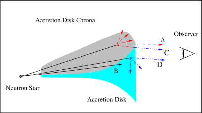
where $\sigma_{\text{T}}$ is the Thomson cross-section and where the bound-free absorption cross sections, $\sigma_{\text{bf}}$, are those used in the tbabs model of XSPEC (Wilms et al. 2000). For the fitting the absorption and scattering part in Eq. (2) uses the same $N_{\text{H}}$. For the Thomson scattering part in Eq. (2) the electron density calculates from $N_{\text{H}}=1.21\,N_{\text{e}}$, assuming material of solar abundances (Wilms et al. 2000). The constant $C$ in Eq. (2) defines the relative ratio of absorbed and scattered radiation to the unaffected radiation. A larger value of $C$ implies a larger degree of absorbed and scattered flux. During the remainder of this paper the unaffected model component will be called MC I and the component influenced by absorption and Thomson scattering will be referenced as MC II. For the model component MC I we neglected Galactic absorption since the Galactic $N_{\text{H}}=1.79\,10^{20}\,\text{cm}^{-2}$ is small compared to the $N_{\text{H}}$ of model component MC II. A schematic picture illustrating the geometric situation during the turn-on is shown in Fig. 2. The positions of the accretion disk and an accretion disk corona relative to the neutron star are shown. Photons following beam A, marked by a dashed line, are scattered in the corona and can be partially absorbed in the accretion disk rim (beam C, dash dotted line). While a certain fraction of photons are blocked by the accretion disk (beam B), the outer parts of the accretion disk are optically thin for X-rays. Therefore, the spectral distribution of photons following beam D will show strong signature of photoelectric absorption. To simplify matters, photons reaching the observer directly without being modified by either the accretion disk nor the accretion disk corona are not shown in Fig.2. Comparing this geometric interpretation with the spectral model given in Eq. (2) allows the following interpretation:

• The unaffected model component $I(E)=I_{0}(E)+I_{\rm Fe}(E)$, called MC I from now on, accounts for photons following beam A and photons reaching the observer directly (this case is not shown in Fig. 2).

• The model component modified by photoelectric absorption and Thomson scattering $I(E)=a(E)\cdot(I_{0}(E)+I_{\rm Fe}(E))$, called MC II from now on, represents the spectral distribution of photons following beam C and beam D.

We emphasize that it is not possible to use a physically more realistic spectral model which treats scattered, absorbed, and direct flux separately. The problem lies within the nature of Thomson scattering: for photon energies $E\lesssim 10\,\text{ke\kern-0.89996ptV}$ ($E\ll m_{\text{e}}c^{2}$) and when the influence of multiple scatterings can be neglected ($\tau\lesssim 5$), scattering of photons by stationary and free electrons can be treated as elastic and consequently energy independent (classical Thomson approximation). This makes it impossible to separate, e.g., the direct flux and the flux contribution from photons scattered into the line of sight (beam A) using spectral analysis alone.

Figure 3: From top to bottom: (a) $N_{\text{H}}$ [$10^{22}\text{cm}^{-2}$], (b) ratio between the model component MC II and MC I as defined in Eq. (2), and (c) normalization of the iron line $A_{\text{line}}$. The uncertainties are $\pm 1\sigma$.

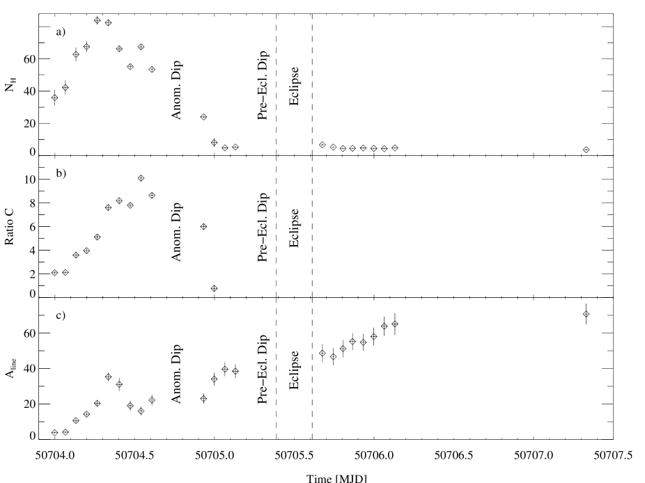
Using this simplified partial covering spectral model all 32 phase averaged PCA and HEXTE spectra were fitted in the energy range $2.9$–$18\,\text{$\text{ke\kern-0.89996ptV}$}$ (PCA) and $15$–$100\,\text{$\text{ke\kern-0.89996ptV}$}$ (HEXTE). In a first iteration we fitted the data with all parameters free except the power-law index $\alpha$ which was kept fixed at $1.068$. This is an average value for $\alpha$ derived from the data with high counting statistics towards the end of the turn-on (orbits 15–31). The results for the remaining free fit parameters are listed in Table 4. This analysis reveals that the folding energy $E_{\text{cutoff}}$, $E_{\text{fold}}$, $E_{\text{cyc}}$, $\sigma_{\text{ cyc}}$, $E_{\text{Fe}}$, and $\sigma_{\text{Fe}}$ show no significant variation over the duration of the turn-on. Therefore, these values were kept fixed at their mean values (see Table 3) for the further analysis. Leaving these values fixed allows us to determine the variation of the remaining free parameters for the time of turn-on, which are the neutral column density $N_{\text{H}}$, the ratio $C$, the normalization of the power law $A_{\text{PL}}$, and of the iron emission line $A_{\text{Line}}$. The results are shown in Fig. 3 and the corresponding fit parameters are given in Table 5.

Table 3: Parameters fixed to their mean value for the fitting of the spectra over the time of the turn-on.

Parameter	Value
$\alpha$	1.068
$E_{\text{cutoff}}$	21.5 keV
$E_{\text{fold}}$	14.1 keV
$E_{\text{cyc}}$	39.4 keV
$\sigma_{\text{cyc}}$	5.1 keV
$E_{\text{Fe}}$	6.45 keV
$\sigma_{\text{Fe}}$	0.45 keV

3.2 Spectral Parameters

Assuming a simple geometrical model of a turn-on where the outer edge of the accretion disk opens the line of sight to the central neutron star as indicated in Fig. 2, the neutral column density $N_{\text{H}}$ is expected to gradually decrease when the flux increases. As can be clearly seen from Fig. 3a, the behavior of observed $N_{\text{H}}$ is contrary to this simple model: As we have already mentioned earlier (Kuster et al. 1999), $N_{\text{H}}$ increases during the first four RXTE orbits, reaches a maximum during orbit 5, and then declines until orbit 17 where it becomes untraceable. This evolution goes in parallel to the degree of scattered and absorbed radiation, $C$, shown in Fig. 3b, which increases until orbit 09 and afterwards starts to decline. The turning point in the progression of $C$ matches almost exactly the maximum of $N_{\text{H}}$. In contrast to $N_{\text{H}}$ and $C$, the normalization of the Fe emission line, $A_{\text{Line}}$ reproduces the progression of the count rate and increases during the whole of the turn on (Fig. 3c). We will come back to the interpretation of this behavior of $N_{\text{H}}$ and $C$ in Sect. 6.

4 Evolution of the pulse profile

4.1 Pulse variation depending on disk phase

Further insight into the physics of the turn-on comes from the substantial changes in shape and amplitude of the X-ray pulse with 35 day phase. One of the earliest studies of these changes was presented by Bai (1981), who observed that the hard central peak and the soft trailing shoulder of the Her X-1 pulse profile are affected differently over the time of the turn-off. He interpreted this effect by a time dependent covering of the two polar emission regions on the neutron stars surface by the inner accretion disk rim and its corona. Since the thickness of the inner accretion disk rim and the neutron star are of the same order of magnitude, they have similar angular size. Consequently, the observed flux from the two neutron star poles can be affected differently in time by the material of the inner disk rim.

Figure 4: Nomenclature for the different features of the Her X-1 pulse profile. This pulse profile is taken from orbit 30 in the energy range of 9.0–13.0 keV.

Building upon this work and on observations of the change of the pulse-profile during the end of the 35 day cycle, Scott et al. (2000) were able to present a refined geometric model explaining these changes in more detail.

4.2 Observed pulse variation

For the following discussion, we use the nomenclature given in Fig. 4 for the various features of the Her X-1 pulse profile. Fig. 5 shows how the relative strength of these features change with energy. The most distinct variation apparent, is the decreasing flux of the soft leading shoulder with increasing energy. This change leads to a double peaked structure consisting of the hard central peak and the soft leading shoulder that clearly can be identified in the energy range 6–12 keV (Deeter et al. 1998).

During the early phases of the turn-on, strong photoelectric absorption and Thomson scattering will modify the pulse shape (Fig. 6). Thomson scattering in a hot plasma causes the broadening of the pulse profile in all energy bands which leads to an almost sinusoidal pulse shape during early times of the turn-on (orbits 00–05). During later phases of the turn-on (orbits 05–09) only the lowest energy channels are affected by strong noise. This implies that during this phase energy dependant photoelectric absorption is the dominant process. The behavior during orbits 05–09 is very similar to the situation in orbits 10–14 during which the anomalous dip took place, which is presumably caused by cold material located at the outer rim of the accretion disk, crossing the line of sight to the neutron star (Shakura et al. 1999). During the eclipse phase (orbit 21–22) all energy channels are affected by strong noise and no pulsation was detected.

Figure 5: Energy dependence of the pulse profile. The pulse profile of orbit 31 is shown in eight different energy bands. All profiles are normalized to unity. Each profile, except the profile of the energy range 2.0–3.6 keV, is shifted by 0.5 in the $y$ direction relative to the previous profile. Note, the energy dependant change of the relative intensity of the soft leading shoulder to the hard central peak, which results in a double peaked structure close to pulse phase 1.0. This feature is most pronounced at energies between 10–14 keV

.

Figure 6: Evolution of the pulse profile as observed over the time of the turn-on. All profiles are normalized to unity at the maximum of the main pulse, after subtraction of the off-pulse constant flux. Pulse phase 0 is defined as the maximum of the main pulse in the energy band of 13–19 keV.

Figure 7: Pulsed fraction over the time of the turn-on in different energy ranges. To determine the pulsed fraction the pulse profiles have to be smoothed to reduce Poisson noise. The pulsed fraction is given as percentage of the pulsed flux compared to the non pulsed flux.

These effects of scattering and photoelectric absorption can also be seen in the behavior of the pulsed fraction with time (Fig. 7). It is clearly visible that $F_{\text{ pulsed}}$ increases more rapidly in the high energy bands. At lower energies, the pulsed flux is suppressed towards the beginning of the turn-on, similar to the situation observed during egress of the anomalous dip, where the pulsed flux increases faster at higher energies. At the end of the turn-on, after orbit 23, the pulsed fraction is almost constant. Contrary to later phases of the main-on and the turn-off the intrinsic pulse shape does not change significantly over the time of the turn-on. This result is in agreement with earlier findings of, e.g., Gruber et al. (1980), Bai (1981), Trümper et al. (1986), or Deeter et al. (1998). The pulse profile observed at the beginning of the turn-on can be interpreted, therefore, as a main-on pulse profile modified by the influence of photoelectric absorption and scattering.

5 Simulating pulse variation

To quantify the effects of scattering and photoelectric absorption on the change of the X-ray spectrum and the pulse profile shown in Sects. 3 and 4, we now turn to Monte Carlo simulations of the radiation transport of the pulsar’s flux in a scattering medium. For the simulations we assume that the pulse shape seen at the end of the turn-on (orbit 30), is the intrinsic pulse shape caused by the emission characteristic of the neutron star and is not changing over the time of the turn-on. Furthermore, we assume that the smearing of the pulse profile and the change in spectral shape at the beginning of the turn-on are solely caused by scattering and photoelectric absorption in the medium covering the line of sight to the neutron star. With these assumptions we can use the pulse profile observed in orbit 30 as a “template” profile and investigate the effects of a scattering and absorbing corona on the pulse shape depending on $N_{\text{H}}$ and the size of the scattering region. This is done via Monte Carlo simulations, as described in the following sections.

5.1 Monte Carlo Simulations

Assuming a point source emitting the intensity $I(t_{0})$ at time $t_{0}$, the intensity at infinity observed at time $t$ can be written as

$$I^{\infty}(t)=\int_{-\infty}^{t}G(t,t_{0})I(t_{0})dt_{0}$$ (4)

where $G(t,t_{0})$ is the scattering Green’s function, i.e., the appropriately normalized solution of the time-dependent equation of radiation transfer through the scattering and absorbing medium for a $\delta$-function pulse of light emitted at time $t_{0}$.

First analytical approaches to determine the Green’s function for scattering in a cold corona were based on the fundamental method developed by Lightman et al. (1981). Brainerd & Lamb (1987), Kylafis & Klimis (1987), and Kylafis & Phinney (1989) found analytical solutions for $G(t,t_{0})$ for simple geometries, such as the diffusion of photons out of a spherical shell surrounding a central point source. For the general case, analytical results are difficult to obtain and one has to resort to numerical solutions instead. Here, we use a modification of the linear Monte Carlo code based on the method of weights (Sobol 1991) that we have previously used to compute $G(t,t_{0})$ for the case of a hot Comptonizing plasma (Nowak et al. 1999). In our simulations we consider Compton scattering (using the Klein-Nishina cross section), photoelectric absorption from material of solar abundance using the cross sections of Verner et al. (1996), and fluorescent line emission (using the fluorescence yields of Kaastra & Mewe 1993). We model the propagation of photons through a plane-parallel slab with thickness $d$ and hydrogen column $N_{\text{H}}$ (corresponding to a certain optical depth for electron scattering, $\tau_{\text{es}}$) that is illuminated by a source at infinity. We consider both, neutral and fully ionized slabs. Output of the simulation is $G(t,t_{0})$ as a function of $N_{\text{H}}$, $d$, and energy band and the angle-dependent photon spectrum of photons leaving the slab. We normalize the time to the light crossing time of the slab.

Figure 8: $G(t,t_{0})$ in the energy range 1.0–70.0 keV for a neutral corona and low optical depths of $\tau_{\text{es}}=0.01$ ($N_{\text{H}}=1.0\,10^{22}\;\text{cm}^{-2}$), $\tau_{\text{es}}=0.14$ ($N_{\text{ H}}=1.25\,10^{23}\;\text{cm}^{-2}$), and $\tau_{\text{es}}=0.44$ ($N_{\text{H}}=2.75\,10^{24}\;\text{ cm}^{-2}$). The peak at $t=1$ is caused by photons crossing the slab without scattering, the break at $t=2$ is caused by photons scattering at most one time before leaving the slab. Inset: Spectrum emerging from the slab for the same columns. Note the emergent fluorescent emission lines for the larger optical depths.

As an example, Fig. 8 shows $G(t,t_{0})$ for a neutral slab with $N_{\text{H}}=1.0\,10^{22}\,\text{ cm}^{-2}$, $1.25\,10^{23}\;\text{cm}^{-2}$, and $2.75\,10^{24}\;\text{ cm}^{-2}$, while Fig. 9 shows the same for a fully ionized slab. For $\tau_{\text{es}}\lesssim 5$ the Green’s function $G(t,t_{0})$ in Fig. 8 and Fig. 9 is dominated by photons crossing the slab on a straight line without being scattered from electrons. These photons contribute to the peak apparent at diffusion times equal to the light crossing time of the slab ($t_{\text{diff}}=1$) and only a small number of photons diffuse out of the slab after this initial peak. For increasing electron optical depth, the number of diffusing photons increases significantly since the mean number of scatterings per photon increases approximately as $\sim$$\tau_{\text{es}}^{2}$. As a consequence, the maximum of $G(t,t_{0})$ moves towards higher diffusion times, until $G(t,t_{0})$ is dominated by photons scattered multiple times ($\tau_{\text{es}}>5$). The energy loss per electron scattering event can be estimated for a $15\,\text{$\text{ke\kern-0.89996ptV}$}$ photon to $\Delta E\approx 0.44\,\text{$\text{ke\kern-0.89996ptV}$}$. This implies that, as soon as the mean number of scattering per photon increases above $\sim$15–20 ($\tau_{\text{es}}\gtrsim 4$), photons of the energy range between 10–20 keV are redistributed to the energy band of 2–10 keV. This redistribution effect is the origin of the changing spectral shape with increasing optical depth visible in Fig. 9 (inset). As a consequence, the cut-off energy moves towards lower energies and a bump at energies between 1–5 keV arises. For even larger optical depths, $\tau_{\text{es}}>10$, this bump slowly vanishes and the flux above 6 keV decreases rapidly. The overall spectral shape is then given by the left most spectrum shown in the top panel of Fig. 9.

Considering a neutral medium, absorption plays the dominant role over the temporal effects of Compton scattering. For a neutral medium with $\tau_{\text{es}}\gtrsim 1$, almost all flux below 10 keV is suppressed. At such optical depths the effects caused by diffusion time are still negligible since the mean number of scatterings per photon is close to unity. Thus, to achieve noticeable changes in beam shape a high fraction of ionized material is needed. On the other hand a high fraction of neutral material only weakly alters the beam shape but reduces the flux at low energies.

Figure 9: $G(t,t_{0})$ for the same spectral distribution as shown in Fig. 8 but for a fully ionized medium and higher optical depths.

Figure 10: Her X-1 pulse profile of orbit 30 (black) transmitted by a fully ionized scattering medium. The electron optical depth varies from top to bottom from $\tau_{\text{es}}=0.5$ to $\tau_{\text{es}}=5.0$. In addition, for each optical depth value the thickness $d$ of the scattering medium is set to $0.02$ (red), $0.02$ (yellow), $0.2$ (blue), and $0.4$ times (dark blue) the light crossing time of the slab.

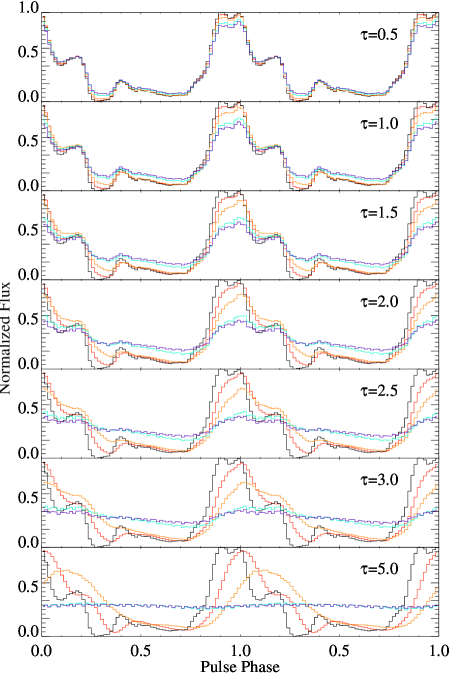
Fig. 10 demonstrates the influence of a fully ionized scattering medium on the pulse shape of Her X-1 for different values of $\tau_{es}$ and a variable thickness of the slab. It is obvious that for large optical depth values ($\tau_{\text{es}}>3$), even a thin scattering layer ($d<0.1$) is sufficient to completely hide the pulse. In addition the structure of the pulse profile is steadily “washed-out” to an almost sinusoidal pulse shape. For $\tau_{\text{es}}<1.5$ the profile’s substructure (soft trailing shoulder) is still apparent even for high values of $d$. Note especially the shift in pulse phase, which is pronounced in the modified pulse profile for $\tau_{\text{es}}>2.0$. This phase shift corresponds to the shift of the maximum of $G(t,t_{0})$ apparent in Fig. 9.

Orbit 05

Orbit 06

Orbit 08

Orbit 09

Orbit 15

Orbit 24

Figure 11: Fit of simulated pulse profiles to observed pulse profiles for the selected observations (compare Fig. 6). The solid line represents the count rate of the observed pulse profile of the indicated orbit, and the dashed line represents the simulated best-fit pulse profile. The residuals of the fits are given at the bottom. All energy bands are fitted simultaneously.

5.2 Analysis of the Pulse Profile

To simulate the variation of the pulse profile during the turn-on we calculated $G(t,t_{0})$ for the same energy ranges we used in Section 4 and each RXTE orbit for two cases:

1. $G_{\text{n}}(t,t_{0})$ for a neutral corona, with $N_{\text{H,n}}\approx N_{\text{H}}$ of the spectral analysis for each single orbit.

2. $G_{\text{ion}}(t,t_{0})$ for a completely ionized corona with $1.0\,10^{22}\,\text{cm}^{-2}\leq N_{\text{H,es}}\leq 9.5\,10^{24}\,\text{cm}^{-2}$.

The Green’s functions $G_{\text{n}}(t,t_{0})$ and $G_{\text{ion}}(t,t_{0})$ can then be compared directly with the spectral model given by Eq. (2). Following the notation introduced in Sect. 3.1, $G_{\text{ion}}(t,t_{0})$ corresponds to the model component MC I and $G_{\text{n}}(t,t_{0})$ to the model component MC II used for the spectral analysis. For a medium where a fraction $f$ is fully ionized, the total Green’s function is given by $G(t,t_{0})=(1-f)\,G_{\text{ion}}(t,t_{0})+fG_{\text{n}}(t,t_{0})$. Using a fixed $G_{\text{n}}(t,t_{0})$ with the respective $N_{\text{H,n}}$ for each orbit from the spectral analysis and variable $G_{\text{ion}}(t,t_{0})$, we can simulate pulse profiles an observer located at infinity would see, by applying Eq. (4) to the “template” pulse profile. As mentioned above, the time scale of the simulated light curves is normalized to the thickness of the corona, i.e., $t-t_{0}$ is measured in units of the light crossing time of the slab. Therefore, Green’s functions for different values of $d$ can be obtained by simply rescaling the time. For our analysis we chose $d$ between 0.1 and 6 light seconds, appropriate for the dimension of the accretion disk in Her X-1 with $r_{\text{in}}\sim 10^{8}$ cm and $r_{\text{out}}\sim 10^{11}$ cm (Cheng et al. 1995). To obtain a proper flux normalization, the integrated flux of the profile of orbit 30 was set to unity. All other simulated pulse profiles are normalized relative to this flux. From the spectral fitting of the partial covering model to the observed spectra, the parameters of the spectral model components MC I and MC II are known. By integrating the differential photon flux of the model spectra over the specific energy bands of Fig. 6, the total flux per energy range can be calculated. Using the integrated photon flux both Green’s functions, $G_{\text{n}}(t,t_{0})$ and $G_{\text{ion}}(t,t_{0})$, can then be normalized to the observed flux according to

$$\int_{t_{\text{0}}}^{t_{\text{1}}}\int_{0}^{\infty}R(h,E)N_{\text{ph}}(E,t)\,dE\,dt=\int_{-\infty}^{t}G_{E_{1},E_{2}}(t,t^{\prime})\,dt$$ (5)

where $N_{\text{ph}}(E)$ is the differential photon flux and $R(h,E)$ the detector response matrix. Finally we performed a $\chi^{2}$ minimization fit of simulated to observed pulse profiles as shown in Fig. 6 for each single RXTE orbit. The different energy ranges were fitted simultaneously. This procedure allows us to determine $N_{\text{H,es}}$, and $d$ as well as their uncertainty.

Figure 12: $N_{\text{H,es}}$ as a function of time determined with the method of pulse profile fitting as described in the text. The error bars are at the $1\sigma$ confidence level.

As an example, the results of the fit of simulated to observed pulses are shown in Fig. 11 for different orbits. The result for the selected orbit demonstrates, that qualitatively and quantitatively the simulation can well reproduce the observed pulses in all energy bands. Similar results can be achieved for observations not shown in Fig. 11. The integrated absolute flux in all energy bands is reproduced with an accuracy $\lesssim 10\%$. For observations earlier than orbit 04 the analysis suffers from the low signal to noise ratio in the observed spectra and a resulting high uncertainty in the normalization of $G_{\text{ion}}(t,t_{0})$ and $G_{\text{ n}}(t,t_{0})$.

Fig. 12 shows the overall development of the electron optical depth over the full turn on. In the figure we give $\tau_{\text{es}}$ in terms of the electron column depth, $N_{\text{H,es}}$, to enable a direct comparison with the results of the spectral fitting. During the early phases of the turn on, $N_{\text{H,es}}$ is very high and the absorbing medium is Compton thick. For the later observations, $N_{\text{H,es}}$ decreases and then levels out at a constant level. These results are a qualitative confirmation of the behavior already expected from the visual inspection of the pulse profile evolution: during the early stages the pulse profile is completely dominated by scattering, while in later stages the direct radiation becomes more and more important. We note, however, that the overall electron column deduced from our Monte Carlo simulations is significantly higher than the column deduced from spectral fitting. Given the explorative character of the Monte Carlo simulations and the simplifications introduced in the model, this is not unexpected. For example, our assumption of the scattering medium being a mixture of either completely neutral or completely ionized is certainly an oversimplification, as is the assumption of a slab geometry. On the other hand, as we will show below, despite these simplifications the overall trend of $N_{\text{H,es}}$ is in agreement with the common models for the 35 day turn-on and thus reduces the ambiguities from the spectral decomposition.

6 Conclusion and discussion

In this paper we have shown that the evolution of the X-ray spectrum and pulse profile during the 35 day turn-on of Her X-1 can be explained by invoking a varying contribution of scattered and heavily absorbed photons to the observed data (Sect. 3 and 5). Using Monte Carlo simulations, in Sect. 5 we showed that the observed behavior of these components appears to be consistent with the results of pulse profile analysis with theoretical Green’s functions for the scattering and photoelectric absorption in the accretion disk. Despite the existing limitations, such as modeling the accretion disk rim by a simple slab with uniform density or modeling the scatterer as either fully ionized or neutral, the methods applied here show that the distinct contributions to the final pulse profile and spectrum can in principle be separated by making use of the smearing of the pulse profile caused by the scattering in the plasma. Our results confirm earlier work based on X-ray spectral analysis alone on the nature of the turn-on of the 35 day cycle and on the nature of the accretion disk of Her X-1 (Davison & Fabian 1977; Parmar et al. 1980; Becker et al. 1977; Burwitz et al. 2001). Our analysis yields an optical depth of $\tau_{\text{es}}\approx 3$–$10$ for the scattering medium which is necessary to explain the observed smearing of the pulse profile. Such optical depths are consistent with coronal models of neutron stars in LMXRBs (e.g., Miller 2000, and references therein).

The behavior summarized above can be explained by a simple geometric model that takes into account the outer rim of an accretion disk that opens the line of sight to the neutron star and the influence of a hot accretion disk corona sandwiching the accretion disk. Fig. 13 shows the positions of the accretion disk, the disk corona, and the location of the observer are shown for different times of the turn-on. The observed PCA spectra corresponding to the phases of the turn-on and the unfolded spectral model components for the energy range $3\leq E\leq 12\,\text{$\text{ke\kern-0.89996ptV}$}$ are shown in the right panel of Fig. 13. The individual components of the spectral model are shown separately.

Figure 13: Schematic view of the outer accretion disk rim (blue), the accretion disk corona (grey), and the neutron star for three different times during the turn-on (not to scale). Right panel: Unfolded PCA spectra and the components of the spectral model for selected orbits. The following components are shown: observed spectrum (solid line), spectral model component MC I (dotted line) and MC II (dashed line), and the Fe line.

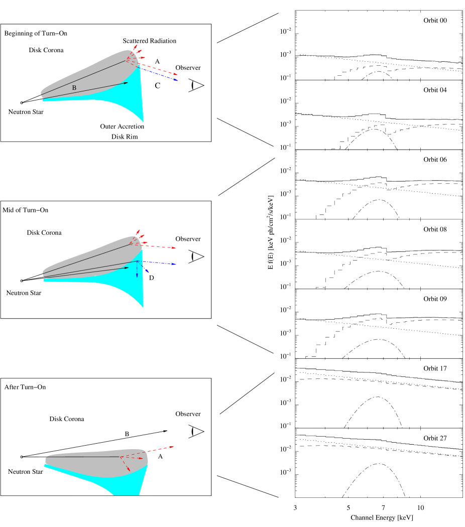
At the start of the turn-on, Thomson scattered radiation from the corona, which is partially absorbed, dominates the observed spectrum. The topmost image of Fig. 13 “Beginning of turn-on” illustrates the orientation of the disk and the location of the observer relative to the disk for this time. Photons following beam A, marked by a dashed line, are scattered in the corona and partially absorbed in the disk rim (beam C). The direct view to the neutron star at this time is still blocked and photons following beam B cannot reach the observer. The corresponding spectra are those observed in orbits 00 and 04. Since the scattered spectral model component MC I dominates the observed spectral flux, only a small fraction of absorbed flux can be detected. As a result, the total observed spectrum, which is the sum of all model components, shows only a weak signature of absorption and low values of $N_{\text{H}}$ are measured. On the other hand, however, those scattered photons which finally reach the observer have undergone many scattering events such that the pulse profile is heavily distorted until orbit 06. In the pulse profile fitting, this phase of the turn-on will therefore be characterized by large values of $N_{\text{H,es}}$.

As soon as the disk starts to open the line of sight to the neutron star (indicated by the downward moving disk in the image “Mid of Turn-On” of Fig. 13), the parts visible of the corona increase and consequently the observed flux in MC I increases as well. In parallel, the apparent absorbed flux increases, because the disk becomes more and more transparent for photons scattered in the corona (beam C). Around the mid point of the turn-on, the outer disk rim starts to become optically thin for photons directly coming from the neutron star following beam D (“Mid of turn-on”). As a consequence the flux in component MC II (the ratio $C$ in Fig. 3) rises more rapidly compared to the flux of MC I. Since MC II determines the curvature of the total observable spectrum, $N_{\text{H}}$ apparently increases. Since the pulse profile due to MC II expected to be far less smeared, pulse profile fitting during this episode will shown a decrease of the overall $N_{\text{H,es}}$. During the further evolution the contribution of MC II continues to increase until it dominates the spectrum. This event takes place right after the turning point in the track of $N_{\text{H}}$ shown in Fig. 3a.

Shortly before the anomalous dip, the apparent $N_{\text{H}}$ rapidly starts to decrease. Both components MC I and MC II are now indistinguishable (orbit 17 and later) because photoelectric absorption and electron scattering become negligible. Based on the interpretation of Cheng et al. (1995), this indicates that a larger amount of photons from the inner parts of the accretion disk close to the neutron star reach the observer. Finally, at the end of the turn-on, the neutron star is directly visible when the main-on starts.

In summary, models as the one outlined above seem to be successful in describing the overall features of the 35 day turn-on of Her X-1. We note, however, that our results in Sect. 5 also show that for very high columns, the separation into two components fails due to low counting statistics during early phases of the turn-on although the overall picture stays consistent. The success of the analysis presented here, however, is a first step towards self-consistently modeling both, the spectral evolution and the timing behavior of Her X-1. Further refinements of the method are still possible, e.g., when taking the absolute phase shift of the observed pulse profile into account and by using more realistic geometries.

7 Acknowledgments

We acknowledge partial funding from DLR grants 50 OX0002, 50 OR0302, DFG grant Sta 173/31-1, and NATO grant PST.CL975254.

Appendix A Results of the spectral analysis

Table 4: Results of the spectral fitting to the Her X-1 turn-on data with all parameters set free, except the parameters where no errors are given for and the power law index $\alpha$ which was kept fix at $\alpha=1.068$.

Obs.	$N_{\rm H}$	$C$	$A_{\rm PL}$	$E_{\rm cut}$	$E_{\rm fold}$	$E_{\rm Fe}$	$\sigma_{\rm Fe}$	$A_{\rm Line}$	$E_{\rm cyc}$	$\sigma_{\rm cyc}$	$\tau_{\rm cyc}$	$\chi^{2}/\rm dof$
	$10^{22}\rm{cm}^{2}$		$10^{-3}$	keV	keV	keV	keV	$10^{-4}$	keV	keV
00	$44.73^{+3.17}_{-7.24}$	$2.14^{+0.14}_{-0.13}$	$4.2^{+0.2}_{-0.2}$	$18.16^{+3.46}_{-2.21}$	$15.4^{+16.6}_{-7.4}$	$6.69^{+0.11}_{-0.14}$	0.77	$4.6^{+0.8}_{-0.7}$	39.7	5.10	$0.50^{+2.58}_{-0.50}$	$77.3/103$
01	$47.34^{+6.14}_{-4.28}$	$2.19^{+0.15}_{-0.12}$	$5.0^{+0.2}_{-0.2}$	$18.24^{+2.21}_{-1.57}$	$9.5^{+5.6}_{-3.3}$	$6.68^{+0.11}_{-0.11}$	0.77	$5.3^{+0.7}_{-0.7}$	39.7	5.10	$0.00^{+2.09}_{-0.00}$	$102.4/103$
02	$56.26^{+4.13}_{-3.65}$	$3.16^{+0.16}_{-0.15}$	$6.1^{+0.2}_{-0.2}$	$18.42^{+3.01}_{-1.69}$	$20.0^{+10.3}_{-7.5}$	$6.60^{+0.09}_{-0.09}$	0.77	$7.6^{+0.8}_{-0.8}$	39.7	5.10	$1.31^{+1.38}_{-1.19}$	$163.7/103$
03	$67.38^{+1.07}_{-7.67}$	$3.57^{+0.16}_{-0.15}$	$8.1^{+0.2}_{-0.2}$	$20.57^{+2.76}_{-2.69}$	$14.3^{+8.8}_{-7.7}$	$6.57^{+0.07}_{-0.07}$	0.77	$11.4^{+0.9}_{-0.9}$	39.7	5.10	$1.61^{+1.71}_{-1.61}$	$134.5/103$
04	$77.35^{+1.81}_{-2.96}$	$4.49^{+0.14}_{-0.15}$	$12.2^{+0.2}_{-0.2}$	$19.98^{+1.45}_{-1.63}$	$11.6^{+3.9}_{-2.8}$	$6.42^{+0.06}_{-0.02}$	0.77	$15.0^{+1.1}_{-1.0}$	39.7	5.10	$0.46^{+0.82}_{-0.46}$	$165.3/103$
05	$75.17^{+1.62}_{-2.39}$	$6.01^{+0.14}_{-0.17}$	$15.2^{+0.2}_{-0.2}$	$21.53^{+1.08}_{-1.08}$	$13.6^{+2.8}_{-2.8}$	$6.54^{+0.07}_{-0.08}$	0.77	$16.5^{+1.4}_{-1.3}$	39.7	5.10	$0.91^{+0.56}_{-0.56}$	$198.9/103$
06	$61.37^{+1.46}_{-1.23}$	$7.15^{+0.13}_{-0.15}$	$17.4^{+0.3}_{-0.3}$	$21.05^{+0.92}_{-0.98}$	$14.5^{+2.4}_{-2.2}$	$6.70^{+0.10}_{-0.10}$	$1.00^{+0.13}_{-0.02}$	$13.4^{+1.8}_{-1.8}$	39.7	5.10	$1.25^{+0.52}_{-0.47}$	$142.7/103$
07	$54.84^{+1.35}_{-1.26}$	$7.70^{+0.17}_{-0.16}$	$17.7^{+0.4}_{-0.4}$	$21.01^{+0.78}_{-0.88}$	$12.0^{+2.2}_{-2.0}$	$6.71^{+0.09}_{-0.12}$	$1.00^{+0.00}_{-0.09}$	$17.7^{+2.7}_{-3.0}$	39.7	5.10	$0.41^{+0.51}_{-0.41}$	$122.2/102$
08	$65.75^{+2.77}_{-0.80}$	$9.94^{+0.31}_{-0.20}$	$14.3^{+0.3}_{-0.3}$	$21.07^{+0.86}_{-0.93}$	$12.9^{+2.2}_{-1.9}$	$6.68^{+0.12}_{-0.11}$	$0.98^{+0.13}_{-0.02}$	$14.7^{+2.3}_{-1.7}$	39.7	5.10	$0.69^{+0.46}_{-0.40}$	$119.8/102$
09	$52.66^{+1.27}_{-1.39}$	$8.37^{+0.17}_{-0.21}$	$17.6^{+0.4}_{-0.4}$	$21.56^{+1.04}_{-1.10}$	$11.3^{+2.6}_{-2.5}$	$6.67^{+0.13}_{-0.15}$	$1.00^{+0.00}_{-0.10}$	$17.1^{+3.0}_{-3.0}$	39.7	5.10	$0.77^{+0.67}_{-0.68}$	$135.1/102$
15	$25.36^{+0.70}_{-0.94}$	$5.75^{+0.13}_{-0.13}$	$25.5^{+0.8}_{-1.4}$	$21.24^{+0.39}_{-0.41}$	$12.9^{+1.0}_{-1.0}$	$6.55^{+0.10}_{-0.10}$	$1.00^{+0.00}_{-0.60}$	$31.6^{+4.2}_{-4.6}$	39.7	5.10	$1.02^{+0.22}_{-0.22}$	$108.2/101$
16	$11.91^{+2.30}_{-2.32}$	$0.70^{+0.25}_{-0.10}$	$98.3^{+1.5}_{-14.2}$	$21.18^{+0.46}_{-0.47}$	$12.6^{+1.1}_{-1.1}$	$6.55^{+0.10}_{-0.11}$	$0.71^{+0.18}_{-0.14}$	$39.2^{+6.8}_{-5.2}$	39.7	5.10	$0.80^{+0.25}_{-0.24}$	$93.1/101$
17	$4.74^{+0.42}_{-0.48}$	1.00	$85.0^{+0.4}_{-0.4}$	$21.24^{+0.46}_{-0.48}$	$12.4^{+1.1}_{-1.1}$	$6.60^{+0.11}_{-0.11}$	$0.72^{+0.18}_{-0.15}$	$41.2^{+6.6}_{-5.5}$	39.7	5.10	$0.77^{+0.26}_{-0.26}$	$98.9/102$
18	$5.17^{+0.45}_{-0.46}$	1.00	$85.3^{+0.4}_{-0.4}$	$21.13^{+0.43}_{-0.44}$	$12.0^{+1.0}_{-1.0}$	$6.63^{+0.11}_{-0.12}$	$0.78^{+0.18}_{-0.16}$	$41.2^{+6.8}_{-5.7}$	39.7	5.10	$0.76^{+0.25}_{-0.25}$	$84.4/102$
23	$6.49^{+0.37}_{-0.50}$	1.00	$100.5^{+3.2}_{-0.4}$	$21.91^{+0.58}_{-0.57}$	$10.8^{+2.2}_{-1.0}$	$6.53^{+0.11}_{-0.13}$	$0.75^{+0.19}_{-0.13}$	$50.4^{+8.3}_{-6.9}$	$40.6^{+0.8}_{-0.9}$	5.10	$2.39^{+3.92}_{-1.41}$	$108.7/101$
24	$5.23^{+0.48}_{-0.38}$	1.00	$103.5^{+0.7}_{-0.5}$	$20.77^{+0.67}_{-0.71}$	$13.7^{+1.6}_{-1.3}$	$6.59^{+0.09}_{-0.10}$	$0.70^{+0.18}_{-0.15}$	$53.3^{+8.7}_{-7.1}$	$39.2^{+1.1}_{-1.0}$	$3.34^{+1.90}_{-1.45}$	$1.48^{+0.96}_{-0.45}$	$122.7/100$
25	$4.30^{+0.43}_{-0.38}$	1.00	$104.8^{+0.7}_{-0.5}$	$21.21^{+0.53}_{-0.48}$	$13.4^{+1.5}_{-1.1}$	$6.62^{+0.09}_{-0.10}$	$0.71^{+0.17}_{-0.15}$	$52.8^{+8.1}_{-7.2}$	$39.7^{+1.0}_{-0.9}$	$5.37^{+2.13}_{-1.50}$	$1.16^{+0.27}_{-0.24}$	$117.7/100$
26	$4.31^{+0.40}_{-0.38}$	1.00	$104.7^{+0.6}_{-0.4}$	$22.06^{+0.38}_{-0.34}$	$11.3^{+1.1}_{-0.9}$	$6.64^{+0.08}_{-0.10}$	$0.78^{+0.17}_{-0.13}$	$58.8^{+8.6}_{-6.7}$	$40.0^{+1.2}_{-1.2}$	$5.18^{+2.85}_{-2.32}$	$0.71^{+0.20}_{-0.17}$	$106.6/100$
27	$4.58^{+0.41}_{-0.39}$	1.00	$110.9^{+0.7}_{-0.5}$	$21.01^{+0.35}_{-0.36}$	$12.8^{+1.3}_{-0.9}$	$6.68^{+0.09}_{-0.10}$	$0.75^{+0.17}_{-0.14}$	$57.2^{+8.4}_{-7.0}$	$40.4^{+0.9}_{-0.9}$	$5.16^{+2.33}_{-1.69}$	$0.95^{+0.19}_{-0.17}$	$110.9/100$
28	$4.36^{+0.36}_{-0.35}$	1.00	$110.5^{+3.9}_{-0.7}$	$21.19^{+0.29}_{-0.29}$	$12.2^{+0.8}_{-0.6}$	$6.65^{+0.08}_{-0.09}$	$0.79^{+0.17}_{-0.15}$	$61.9^{+7.9}_{-7.5}$	$39.1^{+0.8}_{-0.8}$	$4.70^{+1.81}_{-1.33}$	$0.83^{+0.16}_{-0.15}$	$114.6/100$
29	$4.24^{+0.36}_{-0.31}$	1.00	$116.1^{+0.7}_{-0.6}$	$21.40^{+0.33}_{-0.31}$	$12.1^{+1.0}_{-0.6}$	$6.68^{+0.08}_{-0.10}$	$0.83^{+0.18}_{-0.16}$	$65.8^{+7.8}_{-8.2}$	$39.7^{+1.0}_{-1.0}$	$5.59^{+3.31}_{-1.55}$	$0.71^{+0.14}_{-0.13}$	$114.5/100$
30	$4.55^{+0.34}_{-0.41}$	1.00	$118.3^{+0.7}_{-0.5}$	$21.14^{+0.39}_{-0.37}$	$12.7^{+1.2}_{-0.9}$	$6.67^{+0.08}_{-0.08}$	$0.77^{+0.03}_{-0.15}$	$64.3^{+6.4}_{-6.9}$	$39.5^{+0.7}_{-0.7}$	$5.25^{+1.92}_{-1.48}$	$1.05^{+0.20}_{-0.19}$	$119.7/100$
31	$3.48^{+0.37}_{-0.37}$	1.00	$116.6^{+0.5}_{-0.4}$	$21.37^{+0.44}_{-0.46}$	$11.6^{+0.7}_{-0.7}$	$6.59^{+0.07}_{-0.08}$	$0.77^{+0.03}_{-0.13}$	$71.2^{+7.1}_{-7.5}$	$40.5^{+0.7}_{-0.7}$	$1.00^{+6.25}_{-0.00}$	$1.97^{+0.99}_{-1.39}$	$95.8/100$

$N_{\rm H}$: Hydrogen column density, $C$: Relative ratio of absorbed and scattered radiation to the unaffected radiation, $A_{\rm PL}$: Power law normalization, ($\text{photons}\,\text{cm}^{-2}\,\text{s}^{-1}\,\text{keV}^{-1}$ at $1\,\text{$\text{ke\kern-0.80997ptV}$}$), $A_{\rm Line}$: Line normalization ($\text{photons}\,\text{cm}^{-2}\,\text{s}^{-1}$ in the line), $E_{\rm cut}$: Cut-off energy (keV), $E_{\rm fold}$: Folding energy (keV), $E_{\rm Fe}$: Gaussian line energy (keV), $\sigma_{\rm Fe}$: Width of the Gaussian line (keV), $A_{\rm Line}$: Line normalization, $E_{\rm cyc}$: Cyclotron line energy (keV), $\sigma_{\rm cyc}$: Width of the cyclotron line (keV), $\tau_{\rm cyc}$: Depth of the cyclotron line. Uncertainties are at $90\,\%$ confidence level for one interesting parameter ($\Delta\chi^{2}=2.71$).

Table 5: Results of the spectral fitting to the Her X-1 turn-on data for the following parameters: $N_{\rm H}$, $C$, $A_{\rm PL}$, and $A_{Line}$.

Obs.	$N_{\rm H}$	$C$	$A_{\rm PL}$	$A_{\rm Line}$	$\chi^{2}/\rm dof$
	$10^{22}\rm{cm}^{2}$		$10^{-3}$	$10^{-4}$
00	$35.98^{+7.60}_{-1.93}$	$2.10^{+0.16}_{-0.15}$	$\leavevmode\nobreak\ 4.2^{+0.2}_{-0.2}$	$\leavevmode\nobreak\ 3.8^{+0.6}_{-0.6}$	$83.9/108$
01	$42.20^{+6.44}_{-2.63}$	$2.13^{+0.14}_{-0.13}$	$\leavevmode\nobreak\ 4.9^{+0.2}_{-0.2}$	$\leavevmode\nobreak\ 4.1^{+0.6}_{-0.6}$	$112.4/108$
02	$62.80^{+4.71}_{-3.65}$	$3.59^{+0.23}_{-0.21}$	$\leavevmode\nobreak\ 6.1^{+0.2}_{-0.2}$	$10.7^{+1.1}_{-1.1}$	$162.3/108$
03	$67.61^{+4.17}_{-2.60}$	$3.97^{+0.20}_{-0.19}$	$\leavevmode\nobreak\ 8.0^{+0.2}_{-0.2}$	$14.3^{+1.1}_{-1.1}$	$131.1/108$
04	$83.92^{+0.33}_{-4.83}$	$5.11^{+0.21}_{-0.19}$	$11.8^{+0.2}_{-0.2}$	$20.4^{+1.4}_{-1.4}$	$151.1/108$
05	$82.43^{+1.91}_{-2.03}$	$7.61^{+0.28}_{-0.28}$	$13.9^{+0.3}_{-0.3}$	$35.3^{+2.5}_{-2.5}$	$115.5/108$
06	$66.27^{+1.65}_{-1.65}$	$8.19^{+0.26}_{-0.25}$	$16.6^{+0.3}_{-0.3}$	$31.0^{+3.6}_{-3.7}$	$130.4/108$
07	$55.18^{+1.14}_{-1.57}$	$7.80^{+0.18}_{-0.17}$	$17.7^{+0.3}_{-0.4}$	$19.0^{+2.8}_{-2.8}$	$138.9/108$
08	$67.47^{+0.74}_{-2.29}$	$10.10^{+0.25}_{-0.26}$	$14.2^{+0.3}_{-0.3}$	$16.0^{+2.5}_{-2.5}$	$135.3/108$
09	$53.46^{+1.84}_{-1.09}$	$8.64^{+0.22}_{-0.21}$	$17.5^{+0.1}_{-0.4}$	$22.2^{+2.3}_{-3.8}$	$154.4/108$
15	$24.02^{+0.81}_{-0.52}$	$6.00^{+0.30}_{-0.24}$	$24.4^{+1.0}_{-1.1}$	$23.0^{+2.8}_{-2.8}$	$145.7/107$
16	$8.13^{+4.50}_{-0.90}$	$0.77^{+0.50}_{-0.10}$	$94.0^{+1.0}_{-2.2}$	$34.0^{+3.7}_{-3.4}$	$128.7/107$
17	$4.84^{+0.37}_{-0.44}$	$1.00^{+0.00}_{-0.00}$	$85.5^{+0.4}_{-0.4}$	$39.6^{+3.9}_{-3.9}$	$135.6/108$
18	$5.34^{+0.43}_{-0.41}$	$1.00^{+0.00}_{-0.00}$	$85.9^{+0.4}_{-0.4}$	$38.5^{+3.9}_{-3.9}$	$105.6/108$
23	$6.72^{+0.54}_{-0.35}$	$1.00^{+0.00}_{-0.00}$	$101.3^{+0.6}_{-0.5}$	$48.7^{+5.1}_{-5.0}$	$121.9/108$
24	$5.30^{+0.43}_{-0.31}$	$1.00^{+0.00}_{-0.00}$	$104.2^{+0.6}_{-0.5}$	$46.6^{+4.9}_{-4.8}$	$144.1/108$
25	$4.41^{+0.40}_{-0.38}$	$1.00^{+0.00}_{-0.00}$	$105.2^{+4.1}_{-0.4}$	$51.2^{+4.9}_{-4.9}$	$137.4/108$
26	$4.55^{+0.35}_{-0.42}$	$1.00^{+0.00}_{-0.00}$	$105.4^{+0.5}_{-0.4}$	$55.2^{+4.7}_{-4.7}$	$129.3/108$
27	$4.72^{+0.35}_{-0.42}$	$1.00^{+0.00}_{-0.00}$	$111.4^{+0.5}_{-0.4}$	$54.8^{+4.8}_{-4.8}$	$134.8/108$
28	$4.47^{+0.37}_{-0.39}$	$1.00^{+0.00}_{-0.00}$	$111.2^{+0.5}_{-0.5}$	$58.0^{+5.0}_{-5.0}$	$140.9/108$
29	$4.33^{+0.36}_{-0.40}$	$1.00^{+0.00}_{-0.00}$	$116.6^{+0.5}_{-0.5}$	$63.8^{+5.4}_{-5.4}$	$173.8/108$
30	$4.75^{+0.35}_{-0.43}$	$1.00^{+0.00}_{-0.00}$	$156.7^{+17.1}_{-14.1}$	$65.1^{+6.4}_{-5.8}$	$150.2/108$
31	$3.70^{+0.40}_{-0.38}$	$1.00^{+0.00}_{-0.00}$	$117.4^{+0.6}_{-0.5}$	$70.7^{+5.8}_{-5.8}$	$102.9/108$

$N_{\rm H}$: Hydrogen column density, C: Relative ratio of absorbed and scattered radiation to the unaffected radiation, $A_{\rm PL}$: Power law normalization (photons cm^-2 s^-1 keV^-1 at 1 keV), $A_{\rm Line}$: Line normalization (photons cm^-2 s^-1 in the line), the following parameters were fixed: the Gaussian emission line was fixed at 6.45 keV with a width $\sigma$ of 0.45 keV, the cut off energy $E_{\rm cut}$ at 21.5 keV, the folding energy $E_{\rm fold}$ at 14.1 keV, the power law index $\alpha$ at 1.068, and the cyclotron energy $E_{\rm cyc}$ at 39.4 keV with a width of $5.1\,\text{ke\kern-0.80997ptV}$. Uncertainties are at 90% confidence level for one interesting parameter ($\Delta\chi^{2}=2.71$).

References

- Arnaud & Dorman (2002) Arnaud, K. & Dorman, B. 2002, Xspec, An X-ray Spectral Fitting Package, User’s Guide for version 11.2.x, Tech. rep., HEASARC – Laboratory for High Energy Astrophysics – NASA/GSFC, available at http://heasarc.gsfc.nasa.gov/docs/xanadu/xspec/manual/manual.html
- Bai (1981) Bai, T. 1981, Astrophys. J., 243, 244
- Becker et al. (1977) Becker, R. H., Boldt, E. A., Holt, S. S., et al. 1977, Astrophys. J., 214, 879
- Boyd et al. (2004) Boyd, P., Still, M., & Corbet, R. 2004, The Astronomer’s Telegram, 307, 1
- Brainerd & Lamb (1987) Brainerd, J. & Lamb, F. K. 1987, Astrophys. J., 317, L33
- Burwitz et al. (2001) Burwitz, V., Dennerl, K., Predehl, P., & Stelzer, B. 2001, in Two Years of Science with Chandra, Abstracts from the Symposium held in Washington, DC, 5-7 September, 2001.
- Cheng et al. (1995) Cheng, F. H., Vrtilek, S. D., & Raymond, J. C. 1995, Astrophys. J., 452, 825
- Coburn et al. (2000) Coburn, W., Heindl, W. A., Wilms, J., et al. 2000, Astrophys. J., 543, 351
- DalFiume et al. (1998) DalFiume, D., Orlandini, M., Cusumano, G., et al. 1998, Astron. Astrophys., in press
- Davison & Fabian (1977) Davison, P. J. N. & Fabian, A. C. 1977, Mon. Not. R. Astron. Soc., 178, 1P
- Deeter et al. (1998) Deeter, J. E., Scott, D. M., Boynton, P. E., et al. 1998, Astrophys. J., 502, 802
- Giacconi et al. (1973) Giacconi, R., Gursky, H., Kellogg, E., et al. 1973, Astrophys. J., 184, 227
- Gruber et al. (1980) Gruber, D. E., Matteson, J. L., Nolan, P. L., et al. 1980, Astrophys. J., Lett., 240, L127
- Kaastra & Mewe (1993) Kaastra, J. S. & Mewe, R. 1993, Astron. Astrophys. Suppl. Ser., 97, 443
- Katz (1973) Katz, J. 1973, Nature Physical Science, 246, 87
- Ketsaris et al. (2001) Ketsaris, N., Kuster, M., Postnov, K., et al. 2001, in Hot points in Astrophysics
- Kuster et al. (1999) Kuster, M., Wilms, J., Blum, S., et al. 1999, Astrophys. Lett. Comm., 38, 161
- Kylafis & Klimis (1987) Kylafis, N. D. & Klimis, G. S. 1987, Astrophys. J., 323, 678
- Kylafis & Phinney (1989) Kylafis, N. D. & Phinney, E. S. 1989, in Timing Neutron Stars, ed. H. Ögelman & E. P. J. van den Heuvel, NATO ASI No. C262 (Dordrecht: Kluwer), 731–737
- Leahy (2004) Leahy, D. A. 2004, Astronomische Nachrichten, 325, 205
- Lightman et al. (1981) Lightman, A. P., Lamb, D. Q., & Rybicki, G. B. 1981, Astrophys. J., 248, 738
- Maloney & Begelman (1997) Maloney, P. & Begelman, M. C. 1997, Astrophys. J., 491, L43
- Miller (2000) Miller, M. C. 2000, Astrophys. J., 537, 342
- Nowak et al. (1999) Nowak, M. A., Wilms, J., Vaughan, B. A., Dove, J. B., & Begelman, M. C. 1999, Astrophys. J., 515, 726
- Oosterbroek et al. (2001) Oosterbroek, T., Parmar, A. N., Orlandini, M., et al. 2001, Astron. Astrophys., 375, 922
- Parmar et al. (1999) Parmar, A. N., Oosterbroek, T., dal Fiume, D., et al. 1999, Astron. Astrophys., 350, L5
- Parmar et al. (1985) Parmar, A. N., Pietsch, W., McKechnie, S., et al. 1985, Nature, 313, 119
- Parmar et al. (1980) Parmar, A. N., Sanford, P. W., & Fabian, A. C. 1980, Mon. Not. R. Astron. Soc., 192, 311
- Schandl & Meyer (1994) Schandl, S. & Meyer, F. 1994, Astron. Astrophys., 289, 149
- Schandl et al. (1997) Schandl, S., Staubert, R., & König, M. 1997, in AIP Conf. Proc. 410: Proceedings of the Fourth Compton Symposium, 763
- Scott & Leahy (1999) Scott, D. M. & Leahy, D. A. 1999, Astrophys. J., 510, 974
- Scott et al. (2000) Scott, D. M., Leahy, D. A., & Wilson, R. B. 2000, Astrophys. J., 539, 392
- Shakura et al. (1998) Shakura, N. I., Postnov, K. A., & Prokhorov, M. E. 1998, Astron. Astrophys., 331, L37
- Shakura et al. (1999) Shakura, N. I., Prokhorov, M. E., Postnov, K. A., & Ketsaris, N. A. 1999, Astron. Astrophys., 348, 917
- Sobol (1991) Sobol, I. M. 1991, Die Monte Carlo Methode, 4th edn. (Berlin: Deutscher Verlag der Wissenschaften), engl. transl.: The Monte Carlo Method, Chicago: Univ. Chicago Press, 1974
- Tananbaum et al. (1972) Tananbaum, H., Gursky, H., Kellogg, E. M., et al. 1972, Astrophys. J., 174, L143
- Trümper et al. (1986) Trümper, J., Kahabka, P., Ögelman, H., Pietsch, W., & Voges, W. 1986, Astrophys. J., 300, L63
- Verner et al. (1996) Verner, D. A., Ferland, G. J., Korista, K. T., & Yakovlev, D. G. 1996, Astrophys. J., 465, 487
- Vrtilek & Cheng (1996) Vrtilek, S. D. & Cheng, F. H. 1996, Astrophys. J., 465, 915
- Vrtilek et al. (1994) Vrtilek, S. D., Mihara, T., Primini, F. A., et al. 1994, Astrophys. J., Lett., 436, L9
- Wilms et al. (2000) Wilms, J., Allen, A., & McCray, R. 2000, Astrophys. J., 542, 914
- Wilms et al. (1999) Wilms, J., Nowak, M. A., Dove, J. B., Fender, R. P., & di Matteo, T. 1999, Astrophys. J., 522, 460