Light-cone Simulations: Evolution of dark matter haloes

We present a new fast method for simulating pencil-beam type light-cones, using the MLAPM-code (Multi Level Adaptive Particle Mesh) with light-cone additions. We show that by a careful choice of the light-cone orientation, it is possible to avoid extra periodicities in the light-cone. As an example, we apply the method to simulate a 6 Gpc deep light-cone, create the dark matter halo catalogue for the light-cone and study the evolution of haloes from $z=6$ up to the present time. We determine the spatial density of the haloes, their large-scale correlation function, and study the evolution of the mass function. We find a surprisingly simple relation for the dependence of halo maximum mass on redshift, and apply it to derive redshift limits for bright quasars.

1 Introduction

The recent (completed and on-going) galaxy redshift surveys (e.g. LCRS, 2dFGRS, 6dF, SDSS) of our local universe have enormously increased our knowledge of galaxies and of their large scale distribution. These large-scale structure data sets provide also a powerful tool for breaking many of the parameter degeneracies associated with the CMB data (Spergel et al. sper (2003)). Clusters of galaxies, the largest virialised systems known, have a vital role in understanding cosmological structure formation. In particular, following the evolution of clustering with redshift, we can put direct constraints on models for the evolution of density perturbations (Munshi et al. mun (2004)).

However, it is impossible to study cosmological evolution, using only such local surveys. Thanks to recent developments in instrument technology there are several new surveys designed to probe at increasingly higher redshifts, in order to study the early evolution of galaxies and their systems. We shall list a few of them.

The DEEP2 redshift survey is planned to study the evolution of properties of galaxies and the evolution of the clustering of galaxies from $z\sim 1.5$ to $z=0$, using the DEIMOS spectrograph on the 10 m Keck II telescope. The results will be compared with those of the local surveys, e.g., as the LCRS (Coil et al. Coil (2002)). The ALHAMBRA photometric survey (Moles et al. moles05 (2005)) has similar goals. It will cover 4 square degrees of sky, and will find galaxies up to redshifts $z\approx 5$.

The VIRMOS galaxy redshift survey, using VIMOS on the VLT telescope, is also designed to study the formation of galaxies and large-scale structure over the redshift range ($0<z<5$), covering sixteen square degrees of the sky in four separate fields (Virmos Consortium, http://www.oamp.fr/virmos/).

GOODS (the Great Observatories Origins Deep Survey) aims to unite extremely deep multi-wavelength observations (up to $z\approx 6$) both from ground-based (VLT, Keck, Gemini, NOAO, Subaru) and space telescopes: Hubble (HST Treasure program), SIRTF (Legacy Program), and Chandra. Observations cover two fields ($10^{\prime}\times 16^{\prime}$), centered on the Hubble Deep Field North and the Chandra Deep Field South. The primary goal of the GOODS program is to provide observational data for tracing the mass assembly of galaxies throughout most of cosmic history (Dickinson & Giavalisco dic (2003)).

The Galaxy Evolution Explorer (GALEX) satellite was launched in 2003 (Martin et al. m05a (2005)). In combination with ground based optical observations this satellite allows to study the star formation rate, the galaxy luminosity function and other parameters of galaxy evolution over the redshift range $0<z<5$, and even beyond this limit (see http://www.galex.caltech.edu).

Several recent studies have revealed clustering of Ly alpha objects, quasars and radio galaxies at very high redshifts (Ouchi et al. ouch (2004), Venemans et al. ven (2004), Malhotra et al. mal05 (2005), Wang et al. wang05 (2005), and Stiavelli et al. stia05 (2005)). For example, Ouchi et al. (ouch (2004)) reported about the discovery of primeval dense structures at redshift 6 containing Lyman alpha emitters (LAEs). Ouchi et al. estimated that masses of these structures - progenitors of present-day large scale structures are of order of $10^{12}M_{\sun}$ - $10^{13}M_{\sun}$ and dimensions are less than 10 $h^{-1}$ Mpc.

By these surveys, observations are reaching the scales where the evolution of galaxies along the light-cone plays an essential role. Comparison of deep surveys with our theoretical understanding of structure formation and evolution has become even more topical and thus simulations, or mock catalogs, have become an important tool for the design of observational projects and for later data analysis. A properly constructed simulation can allow us to compare the observations directly with modern models of structure formation, can serve to test the data processing algorithms for biases, and to quantify the impact of numerous observational selection effects (Yan et al. yan (2004)).

We believe that light-cone simulations mimic better the observational datasets than conventional simulations at $z=0$, and at different “snapshots” at fixed redshifts. The light-cone algorithm stores ’light-cone particles’ on-the-fly, allowing us to follow continuously the evolution of structure. Although not difficult in principle, light-cone simulations tax heavily computer resources – the volumes are too large to model them with necessary mass resolution. The best-known light-cone, “the Hubble simulation” (Colberg et al. colberg (2000)), was run on specialised parallel shared-memory computers, and remains the only one with publicly available data.

The goal of this paper is to present a new method to perform light-cone simulations of deep pencil beams, typical for deep surveys. Our method is rather efficient and allows to perform and analyse the simulation on single workstations. We shall build a light-cone from $z=0$ to $z=6$ in a “concordance” cosmological model, and shall follow the evolution of dark matter (DM) haloes with the cosmic epoch. Visualizations of DM-haloes in the light-cone model can be seen at Tartu Observatory web pages (http://www.aai.ee/$\sim$maret/lc.html).

When our project was almost finished we learned that a similar light-cone project MoMaF has been realized by Blaizot et al. (blaizot05 (2005)). Below we shall compare their approach with ours.

2 The light-cone simulation

2.1 Method

We use the Multi Level Adaptive Particle Mesh code (MLAPM, Knebe et al. knebe (2001)) with light-cone output. The MLAPM code is adaptive, with sub-grids being adaptively formed in regions where the density exceeds a specified threshold. There are similar codes, as the ART code, Kravtsov et al. (kratso (1997)); it is essential that simulations are done with different codes, to cross-check the results of the complex dynamics of the cosmic structure formation.

We base the light-cone on periodic replicas of our simulation cube. This could, of course, introduce extra periodicities in the results, but we shall demonstrate that a clever choice of the light-cone parameters will avoid those, at least for pencil-beams. If we choose the pencil-beam along one of the coordinate axes, we will sample the same regions of the cube many times; but if the direction of the beam is oblique, and the beam narrow, we will use different regions of the cube along the beam.

In order to collect the light-cone, we find first the co-moving light-cone radius and determine all the copies of the original simulation cube, which intersect with the spherical surface of that radius (cover it). For the simplest geometries (almost full-sky) that is enough, but for a pencil-beam patch geometry we have to use three additional checks:

1. find if the cube copy vertices lie inside the patch;

2. find if the patch edges intersect the copy’s faces;

3. find if the patch planes intersect the copy’s edges.

If nothing this happens, the copy-cube does not include the light-cone. This cube list may seem to be an unnecessary complication, but it will speed up light-cone processing for the most interesting deep and narrow light-cones.

When the cube list is completed, we check for all particles their positions in all the candidate cubes, and if the (copy) particle has crossed the light-cone between the preceding $z$ and the present $z$, we find the crossing redshift and coordinates by linear interpolation. Then we check for the patch geometry, if necessary, and write the (copy)-particle data.

Detailed instructions on generation of the light-cone simulations can be found in the MLAPM user guide (http://www.aip.de/People/AKnebe/MLAPM).

The MoMaF project (Blaizot et al. blaizot05 (2005)) takes a slightly different approach, saving first a large number of snapshots and using these later to build the light-cone. When assembling the light-cone, they randomly rotate the snapshots, in order to eliminate the influence of periodicities. As this destroys the continuity of the structure, we prefer not to scramble our cubes. In fact, MoMaF allows such an approach too, for pencil-beam surveys, although Blaizot et al. (blaizot05 (2005)) devote most of their attention to the scrambled case.

2.2 Application

We simulate a pencil-beam mock survey, similar to the contemporary observational surveys. We use a simulation with $256^{3}$ dark matter particles in a $256^{3}$ grid. We follow the evolution from $z=6$ to present time. Our simulation covers $2^{\circ}\times 0.5^{\circ}$ in the sky.

We use a flat cosmological model with the parameters derived by the WMAP microwave background anisotropy experiment (Bennett et al. bennet (2003)): the dark matter density $\Omega_{m}=0.226$, the baryonic density $\Omega_{b}=0.044$, the vacuum energy density (cosmological constant) $\Omega_{\Lambda}=0.73$, the Hubble constant $h=0.71$ (here and throughout this paper $h$ is the present-day Hubble constant in units of 100 km s^-1 Mpc^-1) and the rms mass density fluctuation parameter $\sigma_{8}=0.84$.

The initial data for our simulation was generated in a cube of 200 $h^{-1}$ Mpc co-moving size, for $z=30$. Thus, each particle has a mass of $3.57\cdot 10^{10}h^{-1}\mbox{M}_{\sun}$. The transfer function for our model was computed using the COSMIC code by E. Bertschinger (http://arcturus.mit.edu/cosmics/).

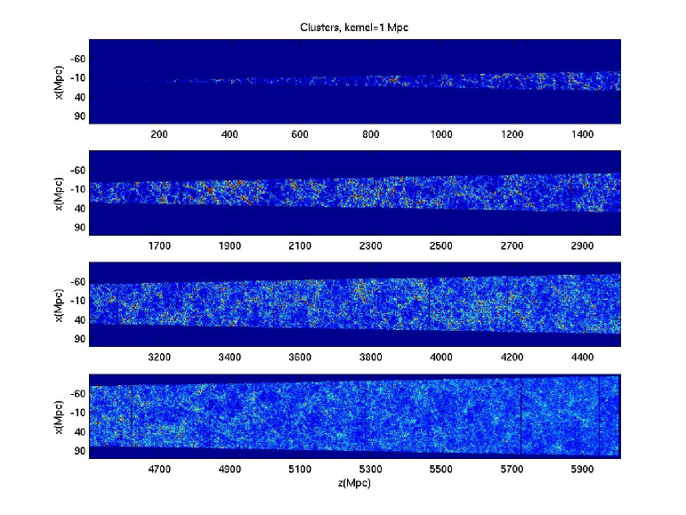
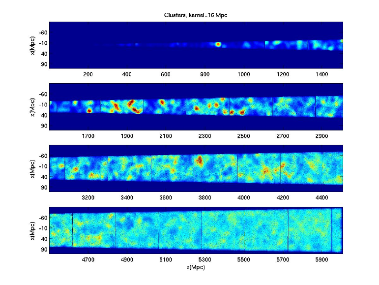
Figure 1: The density field of the 6 Gpc deep dark matter light-cone simulation smoothed with a $r=1.0$ $h^{-1}$ Mpc kernel (upper panels), and with a $r=16.0$ $h^{-1}$ Mpc kernel (lower panels).

Figure 1 shows the projected (dark-matter) density fields of our light-cone simulation from $z=0$ to $z=6$ (for the cosmological model chosen $z=6$ corresponds to 5981.42 $h^{-1}$ Mpc. The density was calculated, using an Epanechnikov kernel ($h(x)\sim(1-x^{2}/r^{2})$ of radii $r$ 1.0 $h^{-1}$ Mpc, 16.0 $h^{-1}$ Mpc - i.e., for the characteristic scales of clusters and superclusters of galaxies.

The full amount of light-cone data (positions and velocities of dark matter particles) can have enormous. The evident way to compress the data is to extract catalogues of dark matter haloes; this are the objects that can be associated with observed galaxies and clusters of galaxies.

As the amount of data is large, we used the simplest algorithm (friends-of-friends, FOF) to identify dark matter haloes. The simulations reported in this paper were run in early 2004; now we would have used a new feature of MLAPM, its halo finder (see Gill et al. gill04 (2004)) that uses the basic adaptive density tree of the simulation, and outputs haloes at all required snapshots. It should not be difficult to adapt that to output light-cone halo catalogs on the fly; this remains to be done. Deep light-cones generate huge amounts of data, and the only practical way to handle this is to keep only the haloes.

FOF uses a linking length $b$ to collect particles in groups with spacing closer than $b$ times the mean inter-particle spacing. The linking length is frequently determined from the virialisation density $\rho_{v}$ (see Bryan and Norman bry (1998)), obtained from the solution for the collapse of a spherical top-hat perturbation. The density $\Delta_{c}$ dependence on background cosmology via the matter density parameter

$$\Omega_{M}(z)=\Omega_{0}(1+z)^{3}/E(z)^{2},$$

where

$$E^{2}=\Omega_{0}(1+z)^{3}+\Omega_{R}(1+z)^{3}+\Omega_{\Lambda}.$$

Bryan and Norman bry (1998) give an approximate formula for that:

$$\Delta_{c}=\rho_{v}/\rho_{\mbox{crit}}=18\pi^{2}+82x-39x^{2},$$

where $x=\Omega_{M}(z)-1$ and $\rho_{\mbox{crit}}$ is the density in the Einstein-deSitter model ($\Omega_{\Lambda}=0,\Omega_{M}=1$). The actual mean density is $\Omega(z)\rho_{\mbox{crit}}$. Thus the linking length that would select virialised haloes at a given redshift $z$ can be written as $b=(\Omega_{M}(z)\Delta_{c})^{\frac{1}{3}}$.

The assumption that objects populate only virialised haloes could be a bit extreme. We normalised the linking length by its present value, comparing the amplitude of the simulated halo mass function (at it’s massive end) with an observational mass function of galaxy groups of the Las Campanas Loose Groups of Galaxies, hereafter LCLG, Heinämäki et al. (hei03 (2003)). In order to obtain this mass function, we ran the MLAPM code in the snapshot mode, with the same initial data we used for the light-cone simulation.

Using this normalisation, we chose the present epoch ($z=0$) linking length as $b=0.23$ (in units of the mean particle separation), which corresponds to the matter density contrast $\delta n/n=80$. This is somewhat lower than the virial density, but not much, and delineates well galaxy groups, as seen in the LCLG Catalog (Tucker et al. tucker (2001)).

Figure  2 shows how the linking length we used changes with redshift. Due to the accelerated expansion at later epochs the haloes need higher density contrasts (and smaller linking lengths) for virialisation.

Figure 2: The FOF linking length as a function of redshift, for the light-cone simulation.

We extracted several populations of dark matter haloes from our light-cone: haloes with 2 or more particles ($M_{h}\geq 7.1\cdot 10^{10}h^{-1}\mbox{M}_{\sun}$), haloes with more than 20 particles ($M_{h}\geq 7.1\cdot 10^{11}h^{-1}\mbox{M}_{\sun}$), and a conservative sample of haloes with more than 100 dark matter particles ($M_{h}\geq 3.6\cdot 10^{12}h^{-1}\mbox{M}_{\sun}$), We cleaned all the group catalogues, using the virial equilibrium condition $E_{r}=E_{kin}/|E_{pot}|<0.5$ ($E_{pot}$ is the potential energy and $E_{kin}$ – the kinetic energy of a group) for groups to be included in our final group catalogue.

The number of small haloes is considerably reduced by the virial condition, which is natural – many of such haloes are random encounters. From the $n_{\mbox{min}}=20$ halo sample, 6.5% of haloes are rejected, and only a few haloes from the rich halo sample do not satisfy the virial condition. This indicates that the linking length we have chosen does not pick up too many non-virialised objects. The final full halo sample includes about 600,000 haloes, the intermediate sample has 14016 haloes and the sample of rich haloes includes 4088 haloes.

3 Checking for periodicities

Assembling a light-cone from periodic replicas of a simulation cube will lead to several statistical biases. These are thoroughly discussed in Blaizot et al. (blaizot05 (2005)). The main bias comes from scrambling the snapshots; as we do not use scrambling, we bypass this bias.

Another bias is caused by the finite volume of the simulation cube and can be corrected for; Blaizot et al. (blaizot05 (2005)) show how to do that. We can also, in principle, to modify the light-cone by linear large-scale modes; this would allow us to model better correlation functions and number counts.

There is one more effect to worry about – as our light-cone is composed of periodic replicas of a much smaller simulation cube, it could have periodicities at scales of about the cube size. The easiest way to check for that is to look at the two-point correlation function of the light-cone. The total number of light-cone mass points is very large; in order to calculate the correlation function we chose the full halo sample, and diluted it randomly, by a factor of six, to keep the $O(N^{2})$ calculation time within reasonable limits. The number of haloes used was about 10,000. We are worried about large-scale correlation, thus we chose the Landy-Szalay estimator, which is one of the best estimator for large scales (see, e.g., Martínez & Saar martsaar (2002)). The rms error of the estimator was taken to be twice the Poisson error. We show this correlation function in Fig. 3.

Figure 3: The large-scale correlation function of DM haloes in the light-cone. The solid line with error-bars shows the correlation function for the whole sample, dotted bars show the correlation function and its 1-$\sigma$ deviation for the redshift interval $z\in[0,1]$.

As we see, no periodicity at scales around 200 $h^{-1}$ Mpc can be seen. The dip in the correlation function at $\sim$50 $h^{-1}$ Mpc and the maximum around $\sim$120 $h^{-1}$ Mpc are real, and are seen both in simulations and in the observed large-scale correlations (e.g., for Abell clusters, Einasto et al. ein97 (1997), see also Einasto et al. ein94 (1994) and Tago et al. tago02 (2002)). A slight indication of periodicity could be seen in the closest redshift interval ($z=0\dots 1$, shown with dotted error-bars). However, even there $\xi(r)=0$ for distances $r>30$$h^{-1}$ Mpc, within $2\sigma$ limits (the volume and the number of haloes are small, and the estimate is rather uncertain). For other redshift intervals the correlation functions practically coincide with the mean for the whole sample.

This can be explained by the good choice of the light-cone geometry. An oblique direction of the light-cone with respect the symmetry axes of the cube will cause the light-cone to sample different regions of the simulation cube in its different replicas. We can quantify this by counting the number of times each cube volume element is included in the light-cone. In order to estimate that, we choose a simple algorithm – we populate the light-cone with a Poisson point process, fold it back onto the original simulation cube, and find the resulting one-point density distribution in this cube. When properly normalised, this distribution approximates the volume multiplicity distribution.

The volume multiplicity distribution for our light-cone is shown in Fig. 4. The two different histograms show the results for two different oversampling factors (the ratio of the density of the Poisson process to the mean light-cone density) – the higher this factor, the better the estimate, and the larger the computer time.

Figure 4: The volume multiplicity histograms of the light-cone.

We see that most of the volume of the simulation cube is used only twice in our light-cone. The worst choice of the light-cone direction, along an axis of the cube, would give a factor close to 30 (the depth of the light-cone divided by the cube size). We can use the mean of the histogram or its rms error as the figure-of-merit $M$ for the volume use; maybe the best choice would be to use a a combination of these:

$$M^{2}=\sigma^{2}_{m}+\bar{m}^{2},$$

where $m$ is the volume multiplicity, and $\bar{m}$ its mean value. Thus, the figure-of-merit for an ideal case (e.g., the Hubble volume $\pi/8$ sterradian light-cone, Colberg et al. colberg (2000)) would be 1; for our light-cone it is 2.9 (but could be over 30). Another relevant characteristic could be the distribution of distances between point replicas. A rough estimate of the mean replica distance for our light-cone is 6000/3=2000 $h^{-1}$ Mpc; this is why we do not see periodicities in the correlation function.

The light-cone figure-of-merit can be found before simulations, and can be used to select the best orientation parameters for a given light-cone geometry (its size and the size of the simulation cube). Its value will also characterise the possible periodicities in the light-cone. We plan to include the figure-of-merit code in the tools section of the MLAPM code package.

4 Evolution: redshift dependence of the dark matter haloes

4.1 Spatial density of haloes

Light-cones as ours can be used for many purposes. As this paper is mainly meant to present the light-cone construction method, we shall give only a few examples below.

First, as our light-cone is pretty deep, we can follow the formation of first massive haloes. Smaller haloes form earlier yet, and their study would require a deeper light-cone.

Figure  5 illustrates the appearance of the first dark matter haloes. In panel (a), DM haloes with masses $M\geq 3.6\cdot 10^{12}\mbox{M}_{\sun}$ are shown. Halos, placed on the density field map (smoothed with 1 $h^{-1}$ Mpc kernel), are marked with black circles. As we see, the very first massive haloes appear at about D=5600 $h^{-1}$ Mpc (z=4.97). Panel (b) shows shows haloes of mass $M\geq 7.1\cdot 10^{11}\mbox{M}_{\sun}$. In this case the very first haloes appear already at $D=5900$ $h^{-1}$ Mpc ($z=5.62$). Smaller haloes exist in our light-cone from its start, $z=6$ already.

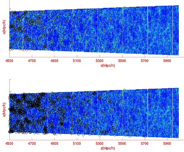
Figure 5: The density field of the simulation. Halos are marked with black circles. The figure shows the most distant part of the light-cone, from 4 to 6 Gpc. The upper panel shows rich haloes ($M\geq 3.6\cdot 10^{12}h^{-1}\mbox{M}_{\sun}$), and the lower panel shows also the intermediate-mass haloes ($M\geq 7.1\cdot 10^{11}h^{-1}\mbox{M}_{\sun}$).

The spatial densities $\rho_{halo}$ of all our DM haloes as a function of redshift (the number of haloes per co-moving volume at redshift bins of width 0.2) for different halo mass limits are shown in Figure  6. Each line indicates different halo mass limits, from $10^{10}\mbox{M}_{\sun}$ (at the top) to $10^{14}\mbox{M}_{\sun}$ (at the bottom of the figure). As can be expected, rich haloes appear later than poor ones. Haloes with masses smaller than $10^{12}\mbox{M}_{\sun}$ exist in our light-cone from the beginning. Overall density evolution of haloes of the two smaller mass ranges is the same; in the redshift range $z=5.7\dots 4$ the spatial density of haloes increases about an order of magnitude. More rapid increase occurs in the redshift interval $z=3.7\dots 3$. These transitions are also seen in the density behaviour of haloes of masses $M\geq 10^{13}\mbox{M}_{\sun}$.

The halo density reaches its maximum at $\sim z=0.9$, after that it decreases. It could be caused by merging of smaller haloes, but could also be a statistical fluctuation, due to the small volume of our pencil beam at redshifts less than one.

The first haloes of mass $M\geq 10^{14}\mbox{M}_{\sun}$ appear at $z\sim 3$. The large variation in their density evolution is due to rareness of such objects and to a small volume of the sample. There is also two overall slopes seen in mass scales less then $10^{14}\mbox{M}_{\sun}$. We also notice that density evolution on almost all mass scales (excepting the the largest mass interval) between z=5.5 and z=3 is more rapid than the later density evolution, between z=3 to z=1. The reason for that could be gradual merging of smaller haloes to form bigger systems.

Figure 6: Spatial density of the haloes as a function of redshift for five different mass limits.

4.2 Halo mass history

Figure  7 shows the cumulative mass function (MF) for dark matter haloes, defined as the number density of haloes above a given mass $M$, $n(>M)$. The solid line shows the mass function for the intermediate mass light-cone haloes ($n\geq 20$). The dotted line shows the MF for a similar halo sample, obtained in our MLAPM simulation, for the final snapshot (a 200 $h^{-1}$ Mpc box at $z=0$). The mass functions differ by an order of magnitude at $10^{11}\mbox{M}_{\sun}$, due to the smaller overall halo density in the deep light-cone. Another difference can be seen at the high mass end of the MF-s – the $z=0$ MF extends to larger masses. This is due to the narrowness of the pencil beam, that occupies only about $10^{-4}$ of the simulation box at $z=0$. Statistics of such surveys should be taken with caution, at least for redshifts less than $z\approx 1$. Without this cosmic variance effect, the light-cone MF should follow the snapshot MF throughout the whole mass range. The dotted line shows the light-cone mass function for all halo masses; this grows steeply, showing that small haloes dominate in number, especially at early epochs, when massive haloes did not exist yet.

Figure 7: The halo mass function for the light-cone (intermediate sample, $n\geq 20$) (solid line) and for a conventional simulation for the present time (dashed). The dotted line shows the light-cone halo mass function for all haloes.

The light-cone can be also used to study the evolution of the halo mass function. We plot this function for different redshift intervals in Fig. 8. The overall shape of the mass functions between $z=0$ to $z=1$ and $z=1$ to$z=2$ is quite similar to the mass function of the whole sample, for the mass interval $M\geq 10^{12}\mbox{M}_{\sun}$ (see Fig. 7). The mass functions steepen with redshift, showing the dominance of small haloes at large redshifts. The characteristic halo masses decrease with redshift, with the maximum halo mass at the largest redshift interval $z=5\dots 6$ being $1.5\cdot 10^{12}\mbox{M}_{\sun}$.

Figure 8: Halo mass functions for different redshift intervals.

The most easier objects to observe at any epoch are the most luminous (most massive) ones. In Fig. 9 we plotted the maximum halo mass for a given redshift. This figure shows that the maximum masses increase exponentially with decreasing redshift, down to the redshift $\sim 0.9$, where the cosmic variance limit appears. This interesting trend, shown in the figure, can be approximated by an intriguingly simple formula

$$M_{\mbox{max}}(z)\approx 10^{15}\mbox{M}_{\sun}10^{-0.5z}\approx 10^{15}\mbox{M}_{\sun}e^{-z}.$$ (1)

This relation is shown by a dashed line in the figure.

5 Early haloes and black holes

As an example of an application of light-cone models, we discuss an interesting possibility that masses of supermassive black holes (BH) may correlate with masses of dark matter (DM) haloes.

Using a sample of 37 local galaxies Ferrarese (fer (2002)) obtained a relation between the masses of BH and circular velocities of galaxy disks, similar to the well-known relation between the‘ BH mass and the bulge velocity dispersion (e.g. Magorrian et al. mag (1998), $M_{BH}/M_{bulge}=3\cdot 10^{-3}$). Using Bullock et al.’s (bul (2001)) simulations (their result $M_{DM}=2.7\cdot 10^{12}(v_{vir}/200\leavevmode\nobreak\ km\leavevmode\nobreak\ s^{-1})^{3}\mbox{M}_{\sun}$ agrees well with our results) together with Ferrarese’s observational results, the best fit for the ratio between $M_{BH}$ and $M_{DM}$ can be written as

$$M_{BH}/10^{8}\mbox{M}_{\sun}\sim 0.10(M_{DM}/10^{12}\mbox{M}_{\sun})^{1.65}$$ (2)

(see figure 5 in Ferrarese’s paper). Ferrarese pointed out (see the references therein) that the critical DM mass for the BH formation could be about $5\cdot 10^{11}\mbox{M}_{\sun}$, while less massive haloes might not offer favorable conditions for BH formation. According to the previous equation, this limits the BH masses by $\sim 10^{6}\mbox{M}_{\sun}$ in such DM haloes. Ferrarese concluded also, that according to the results by Haehnelt et al. (hahn (1998)) only haloes with masses $M\geq 10^{12}\mbox{M}_{\sun}$ may host a black hole with $M_{BH}\geq 10^{6}\mbox{M}_{\sun}$. In our light-cone the spatial density of such host haloes is less than $2\cdot 10^{-7}\mbox{Mpc}^{-3}h^{3}$ at redshifts larger than $z=5.5$.

Figure 9: Masses of the most massive haloes for different redshifts

If we assume that Ferrarese’s $M_{BH}/M_{DMhalo}$ relation also holds at high redshifts, and combine it with our maximum halo mass relation (1), we obtain a simple relation for the BH masses likely to reside in the most massive dark matter haloes as a function of redshift:

$$\frac{M_{BH}}{10^{12}\mbox{M}_{\sun}}(z)=10^{-0.83z}.$$ (3)

McLure & Dunlop (mc (2004)) concluded, based on virial BH mass estimates from the SDSS first release and for 12698 quasars, that quasars’ SBH (super massive black hole) masses lie between $\simeq 10^{7}\mbox{M}_{\sun}$ and $\simeq 10^{9}\mbox{M}_{\sun}$. If we substitute these limits in equation (3), we find that the most prominent quasars exist between the redshifts $\sim 6$ to $\sim 2$. Haloes massive enough to form SBH and hence quasars, either did not exist before the redshift $z\approx 6$, or they were very rare, with the number density $n_{h}<10^{-7}Mpc^{-3}h^{3}$.

6 Conclusions and perspectives

We have presented a new method for simulating pencil-beam type light-cones, using periodic replicas of a base $N$-body cube. Such light-cones are typical for extremely deep optical surveys, either underway or in the planning stage. We have shown that by a careful choice of the light-cone parameters, it is possible to avoid extra periodicities in the light-cone.

We have simulated a deep (up to $z=6$) light-cone, generated the dark matter halo catalogue, and studied its properties. We find that early light-cone is dominated by small haloes, and the maximum halo mass can be clearly traced throughout all the epochs.

We find a simple approximation for the dependence of maximum dark matter halo mass on redshift, and use it to explain the redshift limits of the quasar distribution.

In summary, the algorithm we use to simulate light-cones is lightweight and fast. The code is in the public domain, included in the MLAPM package. Nevertheless, the main bottleneck of any light-cone model is the vast amount of data, proportional to $D^{3}$ ($D$ is the depth of the light-cone). The only way to overcome this is to discard most of the hard-obtained simulation data, the positions and velocities of dark matter particles along the light-cone, and to store only the data on dark matter haloes, creating and analysing them on-the-fly. This could happen soon, as our base MLAPM code already includes the MHF halo finder, which outputs halo catalogues for fixed-time snapshots. Such halo catalogs can be directly used to predict the SZ effect from early galaxy clusters for the Planck mission. Moreover, as gravitational lensing directly traces the total matter density in the universe, our light-cone catalogs are good tools to study the weak lensing of the light emitted by distant quasars, and of the CMB. These are the lines of our present work.

Another important problem in simulating light-cones to compare with observational data is populating dark matter haloes with galaxies, and assigning the galaxies the features an observer sees. In fact, the MoMaF project (Blaizot et al. blaizot05 (2005)) already gives galaxy populations in light-cones, using semi-analytic recipes. We plan to include such recipes in our code, also.

- (1) Bennett, C. L., Hill, R. S., Hinshaw, G., et al. 2003, ApJS, 148, 97
- (2) Blaizot, J., Wadadekar, Y., Guiderdoni, B. et al. 2005, MNRAS, 360, 159
- (3) Bryan, G., Norman, M., L., 1998, ApJ, 495, 80
- (4) Bullock, J. S., Kolatt, T. S., Sigad, Y., et al. 2001, MNRAS, 321, 559
- (5) Coil, A. L., Davis, M., Madgwick, D.S., et al. 2004, ApJ, 609, 525
- (6) Colberg, J. M., White, S. D. M., Yoshida, N., et al. 2000, MNRAS, 319, 209
- (7) Dickinson, M., Giavalisco, M., 2003, in “The Mass of Galaxies at Low and High Redshifts”, Proc. ESO Workshop. eds. R. Bender & A. Renzini; astro-ph/0204213
- (8) Einasto, J., Einasto, M., Frisch, P., et al. 1997, MNRAS, 289, 801
- (9) Einasto, M., Einasto, J., Tago, E., et al. 1994, MNRAS, 269, 301
- (10) Ferrarese, L., 2002, ApJ, 578, 90
- (11) Gill, S. P. D., Knebe, A., Gibson, B. K., 2004, MNRAS, 351, 399.
- (12) Haehnelt, M. G., Natarajan, P., Rees, M. J., 1998, MNRAS, 300, 817
- (13) Heinämäki, P., Saar, E., Einasto, J., et al. 2003, AA, 397, 63
- (14) Knebe, A., Green, A., Binney, J., 2001, MNRAS, 325, 845
- (15) Kravtsov, A., Klypin, A., 1997, ApJS, 111, 73
- (16) Magorrian, J., Tremaine, S., Richstone, D., et al. 1998, AJ, 115, 2285
- (17) Malhotra, S., Rhoads, J.E., Pirzkal, N., et al., 2005, ApJ, accepted [astro-ph/0502478]
- (18) Martin, D.C., Fanson, J., Schiminovich, D. et al. 2005, ApJ, 619, L1
- (19) Martínez, V. J., Saar, E., 2002, Statistics of the Galaxy Distribution, Chapman & Hall/CRC, Boca Raton.
- (20) McLure, R.J., Dunlop, J.S., 2004, MNRAS, 352, 1390
- (21) Moles, M., Alfaro, E., Benítez, N., et al. 2005, astro-ph/0504545.
- (22) Munshi, D., Porciani, C., Wang, Y., 2004, MNRAS, 349, 13
- (23) Ouchi, M., Shimasaku, K., Akiyama, M., et al. 2004, ApJ Lett, [astro-ph/0412648]
- (24) Spergel, D. N., Verde, L., Peiris, H. V., et al. 2003, ApJS, 148, 175
- (25) Stiavelli, M., Djorgovski, S.G., Pavlovsky, C., et al., 2005, ApJ Lett. 622, L1,
- (26) Tago, E., Saar, E., Einasto, J., et al. 2002, AJ, 123, 37
- (27) Tucker, D. L., Oemler, A. Jr., Hashimoto, Y., et al. 2001, ApJS, 130, 237
- (28) Venemans, B.P, Röttgering, H.J., Overzier, R.A., et al., 2004, AA 424, L17
- (29) Wang, J.X., Malhotra, S., Rhoads, J.E., 2005, ApJ Lett. 622, L77, [astro-ph/0502479]
- (30) Yan, R., White, M., Coil, A. L., 2004, ApJ, 607, 739