Multipole vector anomalies in the first-year WMAP data: a cut-sky analysis

Abstract

We apply the recently defined multipole vector framework to the frequency-specific first-year WMAP sky maps, estimating the low-$\ell$ multipole coefficients from the high-latitude sky by means of a power equalization filter. While most previous analyses of this type have considered only heavily processed (and foreground-contaminated) full-sky maps, the present approach allows for greater control of residual foregrounds, and therefore potentially also for cosmologically important conclusions. The low-$\ell$ spherical harmonics coefficients and corresponding multipole vectors are tabulated for easy reference.

Using this formalism, we re-assess a set of earlier claims of both cosmological and non-cosmological low-$\ell$ correlations based on multipole vectors. First, we show that the apparent $\ell=3$ and 8 correlation claimed by Copi et al. (2004) is present only in the heavily processed map produced by Tegmark et al. (2003), and must therefore be considered an artifact of that map. Second, the well-known quadrupole-octopole correlation is confirmed at the 99% significance level, and shown to be robust with respect to frequency and sky cut. Previous claims are thus supported by our analysis. Finally, the low-$\ell$ alignment with respect to the ecliptic claimed by Schwarz et al. (2004) is nominally confirmed in this analysis, but also shown to be very dependent on severe a-posteriori choices. Indeed, we show that given the peculiar quadrupole-octopole arrangement, finding such a strong alignment with the ecliptic is not unusual.

1. Introduction

Since the first-year Wilkinson Microwave Anisotropy Probe (WMAP) data release (Bennett et al., 2003a), a great deal of effort has been spent on analyzing the higher-order statistical properties of the sky maps. This effort has resulted in several reports of both non-Gaussianity and statistical anisotropy (de Oliveira-Costa et al., 2004; Eriksen et al., 2004a, b, 2005; Hansen et al., 2004a, b; Jaffe et al., 2005; Larson & Wandelt, 2004; Vielva et al., 2004), established by means of many qualitatively different methods. Since such findings would contradict the currently popular inflationary based cosmological paradigm, it is of great importance to determine both their origin and significance.

To aid this work, several new methods have been devised. In particular, one method was pioneered by Copi, Huterer & Starkman (2004), who re-discovered a particular decomposition of a given multipole into a geometrically more meaningful set of objects, the so-called (Maxwell’s) multipole vectors. Whereas the standard spherical harmonics expansion is coordinate dependent, these objects are rotationally invariant, providing a somewhat more intuitive interpretation of the object. Specifically, the multipole vector set corresponding to a multipole of order $\ell$ consists of $\ell$ unit vectors and one overall magnitude.

Since the first paper by Copi et al. (2004), several other groups have advanced the method significantly. Choosing a mathematically more stringent approach, Katz & Weeks (2004) and Weeks (2004) both proved uniqueness of the multipole vector decomposition and established efficient methods for computing it. Land & Magueijo (2005) focused on the importance of distinguishing between non-Gaussianity and anisotropy, and introduced the notion of a multipole frame. Finally, a mathematically elegant approach was taken by Slosar & Seljak (2004), who used a Markov Chain Monte Carlo algorithm to map out the complete probability distribution of the low-$\ell$ components, and subsequently used these results to study multipole vector anomalies.

All groups applied their methods to the first-year WMAP data with various results. However, by far most of the effort was spent on analyzing a small set of heavily processed full-sky maps (the WMAP Internal Linear Combination map [WILC] – Bennett et al. 2003a; the Lagrange Internal Linear Combination map [LILC] – Eriksen et al. 2004c; the Tegmark et al. cleaned map [TOH] – Tegmark, de Oliveira-Costa & Hamilton 2003) which are known to have serious problems with residual foregrounds (Eriksen et al., 2004c). In fact, with the exception of the TOH map, the creators of these maps explicitly warn against using them for cosmological analysis.

A notable exception among the analyses quoted above is that of Slosar & Seljak (2004). Their approach is statistically sound, in that it supports partial sky analysis and proper foreground marginalization, but it is also computationally demanding. Its application is therefore somewhat limited. Further, their particular choices and treatment of data make a direct comparison between their results and the ones presented by other groups somewhat unclear.

It should also be noted that Land & Magueijo (2005) did analyze the proper WMAP maps as well, by applying a sky cut to the data directly. However, they did not attempt to reconstruct the full-sky multipole coefficients, and their analysis therefore suffers from multipole mode coupling and increased error bars.

The popularity of the full-sky maps listed above comes from the fact that they appear free of foregrounds by visual inspection. The multipole coefficients may therefore formally be estimated by a straightforward spherical harmonics expansion, without reference to any sky cut and subsequent mode decoupling. Nevertheless, even though it may be difficult to see the foreground residuals by eye, they are certainly present, and an analysis that fully relies on these maps will necessarily be cosmologically dubious. In this paper we address this issue by combining a previously introduced power equalization filter method for estimating the full-sky spherical harmonics coefficients from partial sky data with the ordinary multipole vector method. This allows us to analyze the data frequency by frequency and region by region. In other words, the multipole vector method may finally be used for cosmological studies.

The latter analysis takes a very conservative approach to foreground uncertainties, and, while statistically very robust, the results are not necessarily directly comparable to the ones obtained by other groups, primarily due to choice and treatment of the involved data.

The paper is organized as follows: In Section 2 we briefly review the methods used for both estimating the full-sky harmonics coefficients from cut-sky data, and for computing the multipole vector decomposition from these. Next, in Section 3 we describe the data and simulations used in the analysis. In Section 4 we study the efficiency of the power equalization filter method for reconstructing the multipole components, and compare it with the full-sky cleaning methods. Then we apply our methods to the first-year WMAP data in Section 5, seeking to reproduce earlier claims found in the literature. Concluding remarks are made in Section 6. For easy reference, we also tabulate the low-$\ell$ multipole coefficients for the three cosmologically interesting WMAP Q-, V- and W-bands in Appendix A.

2. Methods and statistics

The following subsections briefly review the methods used in this paper. We refer the interested reader to the original papers for full details; Bielewicz, Górski & Banday (2004) for partial sky analysis by power equalization (PE) filtering, and Copi et al. (2004) for multipole vector decomposition.

2.1. Partial sky analysis by PE filtering

For a given analysis of CMB data to be cosmologically interesting, great care must be taken to exclude non-cosmological foregrounds. In the future it may be possible to perform component separation efficiently, but at present, the only reliable approach is to apply a sky cut and exclude contaminated pixels from the analysis.

While the effect of this operation is transparent in pixel space, it is more complicated in spherical harmonics space, as the spherical harmonics are no longer orthogonal on a cut sky. In order to estimate the full-sky harmonics decomposition from partial sky data, one must therefore decouple the coefficients taking into account the coupling matrix. PE filtering as described by Bielewicz et al. (2004) is one method for doing so.

The first step in this approach is to introduce a new basis set of functions, $\psi$, that is orthogonal on the cut sky (Górski, 1994). In this new basis, the vector of decomposition coefficients, $\mathbf{c}$, is related to the vector of decomposition coefficients of the true signal full sky map $\mathbf{a}$ through the relation

$$\mathbf{c}=\mathbf{L}^{T}\cdot\mathbf{a}+\mathbf{n}_{\psi}\ ,$$ (1)

where $\mathbf{L}$ is the matrix derived by the Cholesky decomposition of the coupling matrix,

$$\mathbf{K} =\mathbf{L}\mathbf{L}^{\textrm{T}},$$ (2)

$$K_{i(\ell,m),j(\ell^{\prime},m^{\prime})} =\int_{\rm{cut\ sky}}Y_{\ell m}^{\ast}(\hat{\mathbf{n}})Y_{\ell^{\prime}m^{\prime}}(\hat{\mathbf{n}})d\Omega_{\hat{\mathbf{n}}},$$ (3)

and $\mathbf{n}_{\psi}$ is the vector of noise coefficients in the $\psi$ basis.

The sky cut causes the coupling matrix $\mathbf{K}$ to be singular, as there is no information in the data about the spherical harmonic modes that lies fully within the sky cut. Hence it is impossible to reconstruct all modes from the $\mathbf{c}$. However, for low-order multipoles, small sky cuts and a high signal-to-noise ratio, it is a good approximation to simply truncate the vectors and coupling matrix at some multipole $\ell_{\rm{max}}$, and then reconstruct the multipole coefficients up to multipole $\ell_{\rm{rec}}$ by filtering of the data vector $\mathbf{c}_{\mathcal{L}}$,

$$\hat{\mathbf{a}}_{\mathcal{L}}=\mathbf{F}\cdot\mathbf{c}_{\mathcal{L}}.$$ (4)

Here the subscript $\mathcal{L}$ denotes the range of indices $i=1,\dots,(\ell_{\rm{rec}}+1)^{2}$, and the filter $\mathbf{F}$ may be chosen to such that the solution $\hat{\mathbf{a}}_{\mathcal{L}}$ satisfy a desired set of conditions. In this paper we will consider the so-called power equalization (PE) filter defined by

$$\left<\hat{\mathbf{a}}_{\mathcal{L}}\cdot\hat{\mathbf{a}}^{T}_{\mathcal{L}}\right>=\left<\mathbf{a}_{\mathcal{L}}\cdot\mathbf{a}^{T}_{\mathcal{L}}\right>.$$ (5)

To construct the filter for the WMAP data we make the usual assumption that both the CMB and noise components are Gaussian stochastic variables. Further, the CMB field is assumed to be isotropic, and the variance of each mode therefore only depends on $\ell$, $C_{\ell}=\left<a^{2}_{\ell m}\right>$. In this paper, we choose the best-fit (to CMB data alone) WMAP power spectrum with a running spectral index (Bennett et al., 2003a; Spergel et al., 2003; Hinshaw et al., 2003) as our reference spectrum. The rms noise level in pixel $p$ is given by $\sigma(p)_{\rm{noise}}=\sigma_{0}/\sqrt{N_{\rm{obs}}(p)}$, where $N_{\rm{obs}}(p)$ is the number of observations per pixel, and $\sigma_{0}$ is the rms noise per observation.

Dependence on the assumed power spectrum might seem to be a disadvantage of this filtering method. However, it was shown by Bielewicz et al. (2004) that the multipole estimation does not depend significantly on the assumed power spectrum in the case of the first-year WMAP data. The same applies to the choice of $\ell_{\rm{rec}}$ and $\ell_{\rm{max}}$. We have chosen $\ell_{\rm{rec}}=10$ and $\ell_{\rm{max}}=30$, but the multipole coefficients do not show strong dependence on these parameters.

2.2. Multipole vector decomposition

The multipole vector formalism was introduced to CMB analysis by Copi et al. (2004), who showed that a multipole moment can be represented in terms of $\ell$ unit vectors and an overall magnitude. As later pointed out by Weeks (2004), the formalism was in fact first discovered by Maxwell (1891). Maxwell showed that for a real function $f_{\ell}(x,y,z)$ that is an eigenfunction of the Laplacian on the unit sphere with eigenvalue $-\ell(\ell+1)$ (i.e., spherical harmonic function $Y_{\ell m}$) there exists $\ell$ unit vectors $\mathbf{v}_{1},\dots,\mathbf{v}_{\ell}$ such that:

$$f_{\ell}(x,y,z)=A^{(\ell)}\nabla_{\mathbf{v}_{1}}\dots\nabla_{\mathbf{v}_{\ell}}\frac{1}{r}\ ,$$ (6)

where $\nabla_{\mathbf{v}_{i}}=\mathbf{v}_{i}\cdot\nabla$ is the directional derivative operator and $r=\sqrt{x^{2}+y^{2}+x^{2}}$. A more useful form of this representation was given by Dennis (2004),

$$f_{\ell}(\mathbf{r})=A^{(\ell)}(\mathbf{v}_{1}\cdot\mathbf{r})\dots(\mathbf{v}_{\ell}\cdot\mathbf{r})+Q.$$ (7)

Here $A^{(\ell)}$ is an overall magnitude, and $Q$ is term fully defined by the components of $\mathbf{v}_{i}$ that include components of angular momenta $\ell-2\ ,\ell-4\ ,\dots$. (This term is needed to take into account the fact that the product of $\ell$ vectors contains terms with angular momenta $\ell-2\ ,\ell-4\ ,\dots$.) Returning to the usual language of CMB analysis, each multipole $T_{\ell}$ may therefore be uniquely expressed by $\ell$ multipole vectors $\mathbf{v}^{(\ell,1)},\ldots,\mathbf{v}^{(\ell,\ell)}$ and a magnitude $A^{(\ell)}$. In the notation of Copi et al. (2004), this reads

$$T_{\ell}(\hat{\mathbf{e}})\equiv\sum_{m=-\ell}^{\ell}a_{\ell m}Y_{\ell m}(\hat{\mathbf{e}})=A^{(\ell)}(\mathbf{v}^{(\ell,1)}\cdot\hat{\mathbf{e}})\dots(\mathbf{v}^{(\ell,\ell)}\cdot\hat{\mathbf{e}})+Q,$$ (8)

where $\hat{\mathbf{e}}$ is the radial unit vector in spherical coordinates. Strictly speaking, the multipole vectors are headless, thus the sign of each vector can always be absorbed by the scalar $A^{(\ell)}$. We will use the convention that all vectors point toward the northern hemisphere.

Algorithms for computing the multipole vectors given a set of $a_{\ell m}$ coefficients were proposed by Copi et al. (2004) and Katz & Weeks (2004). We have implemented the algorithm of Copi et al. (2004) in our codes.

2.3. Multipole vector statistics

Having computed the multipole vectors, we seek to test a given CMB data set with respect to either internal correlations between different multipoles, or external correlations with some given frame. In order to do so, we follow Copi et al. (2004) and define the following set of simple statistics.

The first statistic is based on the dot product, which is a natural measure of vector alignment. Since the multipole vectors are only defined up to a sign, we choose the absolute value of the dot product as our statistic. Second, we also consider cross products of the multipole vectors, $\mathbf{w}^{(\ell,i)}=(\mathbf{v}^{(\ell,j)}\times\mathbf{v}^{(\ell,k)})$ (where $j\neq k,\ j,k=1,\dots,\ell$ and $i=1,\dots,\ell(\ell-1)/2$), in order to test for correlations between multipole planes. Both normalized and unnormalized cross products are considered, the latter corresponding to the oriented area statistic of Copi et al. (2004). Thus, inspired by Copi et al. (2004) and Schwarz et al. (2004), we study the following three statistics for any two multipoles $\ell_{1}$ and $\ell_{2}$ ($\ell_{1}\neq\ell_{2}$):

• $S_{\textrm{vv}}=\sum_{i=1}^{\ell_{1}}\sum_{j=1}^{\ell_{2}}|\mathbf{v}^{(\ell_{1},i)}\cdot\mathbf{v}^{(\ell_{2},j)}|$,

• $S_{\textrm{vc}}=\sum_{i=1}^{\ell_{1}}\sum_{j=1}^{\ell_{2}(\ell_{2}-1)/2}|\mathbf{v}^{(\ell_{1},i)}\cdot\mathbf{w}^{(\ell_{2},j)}|$,

• $S_{\textrm{cc}}=\sum_{i=1}^{\ell_{1}(\ell_{1}-1)/2}\sum_{j=1}^{\ell_{2}(\ell_{2}-1)/2}|\mathbf{w}^{(\ell_{1},i)}\cdot\mathbf{w}^{(\ell_{2},j)}|$.

These are referred to as “vector-vector”, “vector-cross” (or “cross-vector”), and “cross-cross” statistics, respectively.

We use Monte Carlo (MC) simulations to determine the likelihood of these statistics given the isotropic and Gaussian null-hypothesis (see Section 3). As pointed out by Katz & Weeks (2004) and Schwarz et al. (2004), we also note that the multipole vectors of any given multipole is not internally ordered and neither are the dot products. Therefore, the sum of dot products is a better statistic than for instance the $M$ rank-ordered dot products for each multipoles pair, as defined by Copi et al. (2004). We will nevertheless follow the prescription of Copi et al. (2004) in one particular case, to numerically verify their results. For full details on this algorithm, we refer the interested reader to the original paper.

3. Data and simulations

In this paper, we consider the first-year WMAP sky maps (Bennett et al., 2003a) in several forms. Specifically, we analyze both the template-corrected Q-, V- and W-band frequency maps imposing various masks (Kp0, Kp2 – Bennett et al. 2003b; the extended DMR cut, 20+ – Banday et al. 1997) by means of the PE filter method described above, and also four heavily processed (and known to be foreground-contaminated) full-sky maps: the WMAP Internal Linear Combination (WILC) map – Bennett et al. 2003b; the Lagrange Internal Linear Combination (LILC) map– Eriksen et al. 2004c; the Tegmark, de Oliveira-Costa and Hamilton (TOH) map – Tegmark et al. 2003; and the latter from which the Doppler quadrupole term was subtracted – Schwarz et al. 2004. The templates used in the foreground correction process were those described by Finkbeiner et al. (1999), Finkbeiner (2003), and Haslam et al. (1982).

The Doppler term merits some discussion. In principle, this term should be subtracted from all WMAP sky maps prior to analysis. However, its magnitude is very small indeed, smaller than both the map making and foreground induced uncertainties (Hinshaw 2005, private communication), and a result that strongly depends on this term must therefore necessarily be considered somewhat dubious. We choose to subtract this term only from the TOH map, in order to assess its impact.

One goal of this paper is to compare the full-sky ILC method with the partial-sky PE method. The efficiency of each method is assessed through simulation, as we plot the true CMB-only statistic value against the reproduced value after complete processing. The amount of scatter about the diagonal represents the processing-induced uncertainty.

A set of 10 000 ILC simulations were produced using the pipeline described by Eriksen et al. (2004c). For the PE method, we used the simulations described by Bielewicz et al. (2004).

4. Algorithmic efficiency and residual foregrounds

As pointed out in the introduction, the main short-coming of previous multipole vector analyses is the fact that they relied on full sky maps. In this paper we remedy this problem by using the PE filter method of Bielewicz et al. (2004) to estimate the full-sky harmonics components from partial sky data. The goal of this section is to study the relative performance of the PE and the full-sky approaches.

Figure 1.— Comparison of the accuracy of the vector-vector, vector-cross and cross-cross statistics for various methods of the multipoles estimation. The abscissae give the true input values of the statistic for multipoles $\ell_{1}=2$ and $\ell_{2}=3$. The ordinates give output values of the statistic determined after application one of the method. The contours indicate 68% and 95% probability regions as computed from 10 000 simulations. The horizontal lines indicate values of the statistic for the observed WMAP data. In the left column, the lines show the LILC results (solid line), the WILC results (dotted line), and the TOH results (dashed line). In the three remaining columns, the lines show the PE-filter results as obtained from the V-band WMAP sky maps combined with the Kp2 sky cut.

To do so, we apply the above formalism first to 10 000 LILC simulations (Eriksen et al., 2004c), and then to 10 000 PE simulations (Bielewicz et al., 2004). For each single simulation, we also compute the same statistic from the pure CMB input full-sky map, and make a scatter plot of the reconstructed value against the known input value. For a hypothetical method that is able to reconstruct the input CMB field perfectly, all points would obviously lie on the diagonal in such a plot.

Since the PE method supports partial sky analysis, we use the template-corrected WMAP sky maps for our analysis in the next sections. This ensures that residual foregrounds are kept at a minimal level (Bennett et al., 2003b), and the PE simulations are therefore made without including foregrounds. Nevertheless, the real template-corrected maps are certainly not free of residuals, and the direct comparison between the LILC and the PE simulations may therefore be considered somewhat unfair.

To quantify the effect of such residuals, we analyze two additional sets of simulations. For the first set, we add the templates with the amplitudes given by Bennett et al. (2003b) (assuming fixed free-free and synchrotron spectral indices), and then fit for the amplitudes using the approach described by Górski et al. (1996). We then estimate the low-$\ell$ $a_{\ell m}$’s with the PE filtering method. For the second set, we add the templates with 30% of the amplitudes to each simulation, and re-analyze the simulations. Since we do not attempt to correct for the foregrounds at all in this case, the latter set of simulations grossly over-estimates the residual foregrounds present in the template-corrected maps.

The results from these exercises are shown in Figure 1. Left to right columns show 1) the LILC results, 2) the clean PE results, 3) the moderately contaminated PE results, and 4) the heavily contaminated PE results, respectively. Rows show the four different statistics for multipoles $\ell_{1}=2$ and $\ell_{2}=3$ based on normalized cross-products.

Table 1Signal reconstruction efficiency

	Vec-Vec	Vec-Cross	Cross-Vec	Cross-Cross
Pearson’s linear correlation coefficient
LILC	0.750	0.746	0.712	0.698
PE (1)	0.962	0.953	0.955	0.943
PE (2)	0.911	0.904	0.889	0.877
PE (3)	0.811	0.807	0.759	0.754
Standard deviation
LILC	0.325	0.411	0.277	0.355
PE (1)	0.126	0.178	0.109	0.154
PE (2)	0.193	0.253	0.171	0.226
PE (3)	0.281	0.358	0.253	0.321

Note. — The correlation coefficients and standard deviation of the $S$ statistic for the LILC and PE methods. The row marked PE (1) shows results for the PE method applied to clean V-band input maps with Kp2 sky coverage, the row PE (2) shows results for input maps with subtracted foreground templates with fitted coefficients, and the row PE (3) shows results for the input maps with added foreground templates with 30% of the fit coefficients given by Bennett et al. (2003b). (See text for details.)

Clearly, the PE filter approach is superior to the ILC approach. Even in the unrealistic case of 30% residual foregrounds, the scatter is smaller for the PE filter than for the ILC method. Realistically, the PE filter performs somewhat worse than the second column, but slightly better than the third.

We now quantify the scatter observed in each panel both by Pearson’s linear correlation coefficient, and by the standard deviation as measured orthogonal to the diagonal in each plot. The results from these computations are summarized in Table 1. The visual impression from Figure 1 is confirmed by these numbers: the PE filtering method clearly outperforms the ILC method even in the presence of unrealistically strong residuals.

Finally, we take the opportunity to once again emphasize that the full-sky ILC map (and variations thereof) should not be used for cosmological purposes if it is at all possible to avoid. Such maps are highly contaminated by residual foregrounds which are likely to have a significant impact on any moderately sensitive statistic. This is particularly true on large angular scales, such as the ones discussed in this and related papers. The massive scatter seen in the left column of Figure 1 should serve as a clear indication of this fact.

5. Analysis of first-year WMAP data

We now apply our methods to the first-year WMAP data, focusing on three specific claims found in the literature. First, using the multipole vector approach Copi et al. (2004) found some peculiar correlations in the $\ell=3,\ldots,8$ range in the TOH map. These correlations manifested themselves in terms of a number of significant values of the (normalized and unnormalized) $S_{\textrm{cc}}$ statistic. Here we seek to reproduce these results in the official template-corrected WMAP maps using the PE filter method.

Second, numerous authors have reported a strong alignment between the quadrupole and the octopole moments (e.g., de Oliveira-Costa et al. 2004; Copi et al. 2004; Katz & Weeks 2004) using various methods, for instance multipole vector alignments. In Section 5.2 we confirm these findings with our improved method.

Finally, a highly surprising claim was made by Schwarz et al. (2004), who found a nominally strong alignment of the quadrupole and octopole planes with the ecliptic, and even with the vernal equinox. If confirmed real, this finding would suggest that the low-$\ell$ anisotropy pattern seen in the WMAP data could be of a solar system origin. This claim is considered in some detail in Section 5.3.

We note that we have also analyzed our own template-corrected maps (using the method of Górski et al. 1996), and found very similar results as those presented here. Details in the template correction process are therefore not likely to have a major impact on our results, assuming that the templates do indeed trace the real foregrounds satisfactory.

5.1. Internal correlations among the $\ell=2,\ldots,8$ multipoles

The first analysis of the WMAP data based on multipole vectors was performed by Copi et al. (2004). The main conclusion from this work was a claim of correlations among the low-$\ell$ multipoles in contradiction with the currently preferred Gaussian and isotropic cosmological model. This claim was based on two observations. First, the normalized cross-cross multipole vector statistic indicated a very strong correlation between the $\ell=3$ and 8 modes, and second, the unnormalized cross-cross statistic revealed five or eight (depending on likelihood threshold) moderately strong correlations within the $\ell=2$ to 8 modes.

While the nominal significance of their detection was reasonably high (roughly at the 99% level), two problems could be identified with the analysis. First, as subsequently pointed out by several authors (Katz & Weeks, 2004; Schwarz et al., 2004), their statistics were based on a rather elaborate rank ordering scheme with a somewhat unclear interpretation. It is not clear how robust this method is. Second, and more importantly, only the foreground-contaminated WILC and TOH maps were considered in the analysis.

In this paper, we first repeat the original analysis of Copi et al. (2004) based on rank ordering to see if the results (at least nominally) hold when applied to the template-corrected WMAP maps. However, we also analyze the same multipole pairs with the $S$ statistics, in order to study the statistical robustness of the detection. For specifics on the procedure, we refer to Copi et al. (2004); our main target in this paper is robustness with respect to foregrounds, not algorithmic consistency.

The results from the rank ordering analysis are summarized in Table 2. Columns 2 through 5 are to be compared with column 8 of Table 1 of Copi et al. (2004), while columns 6 through 9 are to be compared with columns 10 and 12. While the agreement between our TOH-DQ numbers and their numbers is not perfect, it is quite good overall. Tracking down the cause of the small differences would require having access to both codes; minor details such as the bin size used for estimating the likelihoods do have an impact, in particular on probabilities not in the tails of the distributions. However, we note that we observe perfect agreement with previously published $S$ statistic results (Schwarz et al., 2004; Katz & Weeks, 2004; Weeks, 2004) for all published cases, so all codes appear to be working as expected.

Table 2Low-$\ell$ multipole correlations by rank ordering

		Normalized Cross-Cross					Unnormalized Cross-Cross
$(\ell_{1},\ell_{2})$		LILC	WILC	TOH-DQ	PE		LILC	WILC	TOH-DQ	PE
$(2,3)$		01.73%	05.04%	02.19%	01.45%		01.75%	01.38%	00.11%	03.62%
$(2,4)$		28.16%	55.78%	58.73%	43.21%		25.28%	83.86%	89.44%	57.50%
$(2,5)$		79.97%	77.17%	23.15%	34.36%		99.22%	91.30%	66.77%	76.92%
$(2,6)$		81.53%	88.36%	87.40%	37.27%		64.73%	96.36%	78.55%	19.57%
$(2,7)$		91.08%	99.56%	93.20%	79.47%		91.54%	94.03%	86.24%	68.07%
$(2,8)$		82.55%	60.75%	89.81%	47.06%		67.23%	94.84%	68.29%	28.47%
$(3,4)$		08.28%	06.56%	17.02%	69.95%		14.97%	12.61%	30.85%	70.68%
$(3,5)$		45.95%	70.13%	37.40%	30.05%		58.86%	74.46%	65.30%	64.63%
$(3,6)$		57.59%	46.74%	73.13%	32.75%		75.31%	55.18%	92.67%	70.25%
$(3,7)$		59.28%	70.55%	53.90%	89.17%		86.54%	84.12%	74.25%	75.14%
$(3,8)$		88.47%	86.21%	99.99%	51.26%		97.75%	98.33%	99.75%	52.92%
$(4,5)$		45.67%	48.51%	53.44%	35.19%		70.24%	68.26%	53.26%	37.53%
$(4,6)$		97.59%	86.04%	74.28%	56.19%		87.02%	72.28%	62.90%	40.57%
$(4,7)$		58.15%	97.56%	53.43%	82.42%		24.69%	32.10%	88.82%	98.15%
$(4,8)$		81.16%	88.23%	85.67%	79.73%		86.53%	95.20%	99.00%	69.17%
$(5,6)$		94.28%	99.93%	66.08%	59.03%		95.95%	85.30%	83.88%	24.12%
$(5,7)$		99.70%	95.69%	59.87%	84.32%		98.19%	98.45%	69.04%	95.96%
$(5,8)$		81.17%	78.64%	31.27%	63.85%		30.90%	33.36%	24.40%	76.85%
$(6,7)$		55.27%	59.56%	20.41%	08.19%		63.74%	77.77%	97.42%	16.48%
$(6,8)$		56.28%	80.03%	72.51%	76.98%		48.28%	66.79%	62.53%	51.73%
$(7,8)$		07.99%	18.78%	09.70%	07.69%		10.26%	24.76%	25.11%	05.18%

Note. — Probabilities of obtaining a lower cross-cross statistic value than that observed in the first-year WMAP data, measured relative to MC simulations by means of rank ordering (Copi et al., 2004). The statistics were computed for the LILC, WILC, TOH-DQ, and PE filtered V-band WMAP maps.

As mentioned above, the conclusions of Copi et al. (2004) can be summarized in terms of two different anomalies. First, a high significance was observed for the rank-ordered normalized cross-cross statistic when applied to the $\ell=(3,8)$ pair. This result is confirmed in Table 2, but only for the TOH map. For the other three maps, this particular value is highly insignificant. Therefore, if this detection does signify a real feature, it is only present in the foreground-contaminated TOH map, and not in the more trust-worthy WMAP V-band map. It can therefore not be taken as representative for the first-year WMAP data as a whole.

The second anomaly was defined in terms of an unusually large number of high unnormalized cross-cross values for the TOH map: five out of 21 ranks for the TOH map were found to be larger than 0.9, and eight out of 21 values were larger than 0.8. Once again, we see that this conclusion only hold for the TOH map, and not for the PE-filtered V-band map. Quite on the contrary, the V-band PE filter results appear completely uniform, and no anomalies can be readily identified.

Table 3Low-$\ell$ multipole correlations by dot products

$(\ell_{1},\ell_{2})$	LILC	WILC	TOH-DQ	PE	PE (norm)
$(2,3)$	97.16%	99.29%	99.87%	95.43%	98.82%
$(2,4)$	18.06%	36.71%	34.72%	26.77%	41.30%
$(2,5)$	31.94%	64.20%	51.29%	18.24%	32.34%
$(2,6)$	22.30%	63.83%	62.02%	08.64%	15.88%
$(2,7)$	27.44%	49.98%	79.38%	30.72%	82.54%
$(2,8)$	23.71%	45.93%	76.57%	13.70%	22.63%
$(3,4)$	08.19%	06.31%	11.74%	31.43%	28.21%
$(3,5)$	66.52%	55.50%	55.61%	49.25%	57.42%
$(3,6)$	63.03%	67.86%	71.35%	37.73%	78.77%
$(3,7)$	57.68%	53.91%	66.51%	41.84%	70.52%
$(3,8)$	51.58%	38.07%	47.64%	22.06%	08.36%
$(4,5)$	66.54%	68.05%	75.88%	92.05%	67.29%
$(4,6)$	42.59%	33.51%	57.19%	32.64%	51.10%
$(4,7)$	21.56%	23.02%	46.10%	45.83%	46.38%
$(4,8)$	44.77%	48.59%	57.79%	71.25%	45.38%
$(5,6)$	70.94%	82.05%	79.16%	24.32%	31.81%
$(5,7)$	64.26%	73.48%	77.59%	42.08%	46.88%
$(5,8)$	97.68%	97.32%	97.86%	89.23%	54.70%
$(6,7)$	64.16%	77.42%	64.94%	06.83%	92.13%
$(6,8)$	87.23%	90.25%	73.87%	14.50%	83.13%
$(7,8)$	08.67%	12.84%	30.35%	02.74%	08.11%

Note. — Probabilities of finding a value of the $S_{\textrm{cc}}$ statistic lower than the observed WMAP values, estimated from ensembles of 10 000 MC simulations. The cross-products are all unnormalized (corresponding to the “oriented area” statistic of Schwarz et al. 2004), except for the last column. The PE filter results were obtained from the V-band alone, imposing the Kp2 mask.

Even though the above results appear to refute the original claims of low-$\ell$ correlations, we compute the more robust $S_{\textrm{cc}}$ statistic for the same low-$\ell$ pairs for completeness. The results from these calculations are shown in Table 3. Again, the results appear quite uniform (with the exception of $\ell=(2,3)$, to which we return in the next section), and even the $\ell=(3,8)$ pair does not appear anomalous for any of the maps.

Based on this analysis, we conclude that the results of Copi et al. (2004) are due to a combination of a poorly defined statistic and unreliable data. The anomaly does not survive when subjected to a more careful statistical analysis.

5.2. Quadrupole and octopole correlations

Table 4Quadrupole-octopole correlations

Data	Vec-Vec	Vec-Cross	Cross-Vec	Cross-Cross
Sensitivity to method
LILC	92.04%	2.47%	2.27%	98.57%
WILC	83.28%	2.24%	2.94%	97.31%
TOH-DQ	90.69%	2.03%	1.82%	98.65%
PE	91.36%	1.62%	1.05%	98.82%
Sensitivity to frequency
Q band	93.13%	0.44%	0.45%	99.61%
V band	91.36%	1.62%	1.05%	98.82%
W band	89.28%	1.74%	1.30%	98.73%
Sensitivity to sky coverage
Kp2	91.36%	1.62%	1.05%	98.82%
Kp0	89.66%	2.06%	37.91%	89.92%
20+	90.43%	8.95%	57.92%	81.45%

Note. — Probabilities of finding a value of the $S$ statistic for $(\ell_{1},\ell_{2})=(2,3)$ lower than that of the observed WMAP data for various foreground cleaning methods, frequencies and sky cuts. The default sky mask for the PE filter method is Kp2. The row marked by PE shows results for the PE method applied to the template-corrected V-band WMAP map (see text for details). The cross-products are normalized, following Weeks (2004).

A similar type of anomaly was reported by de Oliveira-Costa et al. (2004). They found that the octopole ($\ell=3$ mode) of the WMAP data spans a plane on the sky, and further, that the normal to this plane is strongly aligned with the quadrupole plane. This anomaly has since then been extensively studied with different techniques (e.g., Weeks 2004; Eriksen et al. 2004c), and is well established by now.

The multipole vector framework is particularly suited for this particular anomaly. Recalling that the multipole vectors of order $\ell$ contain terms of orders $\ell,\ell-2,\ell-4,\ldots$, we see that the quadrupole only consists of a quadratic term plus a constant, while the octopole consists of a cubic and a linear term. Further, it can be shown that the cross-vectors for a given multipole point toward the saddle points of the term of order $\ell$ of each multipole (but, unfortunately, not toward the saddle points of the multipole as a whole.) For the quadrupole, a quite intuitive interpretation of the two multipole vectors is therefore readily available: their cross-product point towards the saddle point. For WMAP, a similar statement is very nearly true for even the three octopole cross-vectors.

Based on these observations, we can make a connection between the multipole vector framework and the approach taken by de Oliveira-Costa et al. (2004); since the WMAP octopole is planar, its saddle points are clustered, and all its cross-products point roughly towards the same point on the sky. Furthermore, since the quadrupole plane is aligned with the octopole plane, even this cross-product points towards the same point on the sky. This is clearly seen in Figure 2, where we plot the positions of the quadrupole and the three octopole cross-product vectors on the sky, in ecliptic projection. Clearly, the four vectors are strongly clustered on the sky, as discussed above.

To assess the estimator uncertainty (i.e., due to the sky cut) in the position of each of the low-$\ell$ cross-product vectors, we used the foreground-free Monte Carlo PE simulations described earlier. For each simulation, we computed the cross-products from both the input map and the reconstructed PE-filtered map (for the V-band alone), and computed the absolute angular distance between the input and output vectors for all possible pairings, and chose the relative ordering with the smallest sum of errors. (This is necessary because the multipole vectors are not internally ordered.) Such computations show that the mean angular error is about $4^{\circ}$ for the quadrupole cross-vector, and 6–$9^{\circ}$ for the three octopole vectors. Thus, the error in each case roughly equals the size of each dot in Figure 2.

Returning to the quadrupole-octopole anomaly, we note that the previously defined $S$ statistics involving cross-products are well suited for measuring the degree of alignment for these two modes, due to the above argument. Following Weeks (2004), we therefore adopt the normalized $S_{\textrm{cc}}$ statistic for this particular analysis, and the corresponding results are tabulated in Table 4.

In the top section, results for different foreground cleaning methods are given. Clearly, the quadrupole-octopole alignment is quite stable (although not perfectly so) with respect to foreground cleaning method: the results for the cross-product type statistics are all at the 98% confidence level, in good agreement with the 98.7% significance obtained using the angular momentum dispersion statistic of de Oliveira-Costa et al. (2004).

In the middle section, we list the same statistic from each of the three cosmologically interesting WMAP frequency bands using the PE filter. Again, the results are very stable, and this gives us confidence that the effect is indeed a feature of the CMB field, rather than caused by residual foregrounds. Further, we also point out that this particular set of results clearly demonstrates the strength of the PE filter method; while the other methods only allow for frequency averaged conclusions, the PE method can provide frequency specific results, and therefore much greater control over foregrounds.

Finally, in the bottom section of Table 4 we give the PE filter results for different sky cuts as applied to the V-band WMAP data. (Here we note that the PE estimator uncertainties for the large 20+ cuts are considerably larger than for the Kp2 and Kp0 masks, as discussed by Bielewicz et al. 2004, and the numbers are only included here for completeness.)

5.3. Ecliptic correlations

Finally, we consider a set of claims made by Schwarz et al. (2004); that the low-$\ell$ anisotropy pattern observed by WMAP could have a very local origin, and that there could be yet unknown microwave sources or sinks within our own solar system. These claims were based on measuring alignments between the multipole vector cross-products for $\ell=2$ and 3 and a pre-defined set of fixed axes. These axes ranged from the somewhat plausible (the super-galactic and ecliptic) to the highly surprising (the equinoxes). Their main result was that the four $\ell=2$ and 3 cross-product vectors were nearly orthogonal to the ecliptic north-south axis, as measured by the dot product. This can visually be seen in Figure 2, as the dots all lie along the equator in the ecliptic frame, and, indeed, clustered near the vernal equinox.

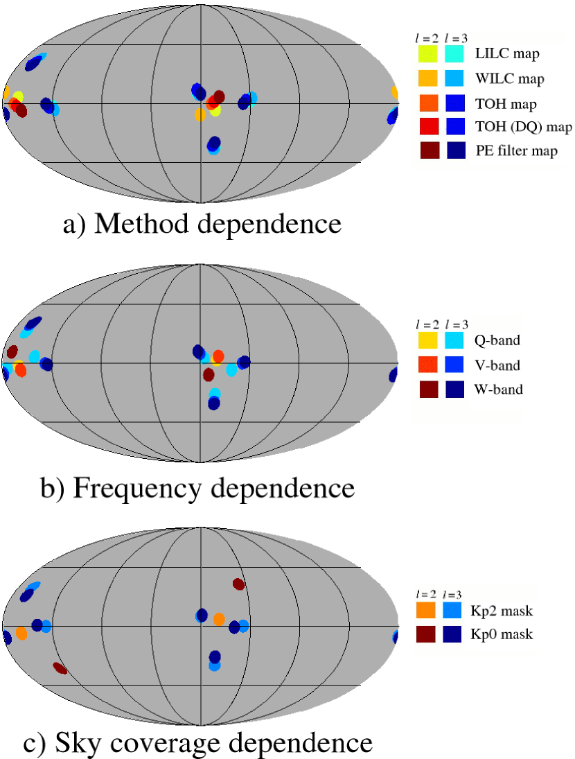
Figure 2.— Multipole cross-product vectors on the sky as a function of cleaning method (top panel), frequency band (middle panel) and sky coverage (bottom panel). Default options for the PE filter results are the V-band map and Kp2 sky cut. The maps are shown in the ecliptic reference frame with the vernal equinox at the center. The radius of each dot is $5^{\circ}$.

We now repeat the calculations of Schwarz et al. (2004), applying the PE filter method to the Q-, V- and W-band WMAP maps, and imposing the Kp2, Kp0 and 20+ sky cuts. We compute the sum of dot products between the ecliptic north-south axis and the union of the $\ell=2$ and 3 cross-product vectors, following Schwarz et al. (2004), and also for each mode individually, up to $\ell=6$. The results from these computations are summarized in Table 5.

Again starting with the top section, we see that the numbers (except for the quadrupole alone) are not very sensitive to the particular foreground correction method. Further, for the particular combination in question ($\ell=2$ and 3), the alignment is in fact stronger for the PE filtered V-band map than for the more contaminated maps (although this may be somewhat of a coincidence, looking at the $\ell=2$ and 3 numbers individually). The numbers also do not depend strongly on frequency or sky cut. As far as these numbers are concerned, the alignment must therefore be assumed to be of CMB origin, and not of foreground origin. Taken at face value, these results therefore appear to confirm the claims made by Schwarz et al. (2004).

However, while the nominal significance of the results seems solid, a much more fundamental objection may be raised against this detection, namely its strong dependence on a-posteriori choices. Two particular problems may be identified, namely the choice of multipoles to include, and the choice of external axis.

In the first case, we see in Table 5 that the ecliptic alignment is only significant if one takes into account both $\ell=2$ and $\ell=3$ simultaneously, and no other multipoles. Further, the quadrupole-ecliptic alignment alone is only significant in the TOH map, and quite insignificant in the PE filtered map. In fact, the numbers for the quadrupole alignment (both for different methods and for different frequencies) imply that a significant amount of foreground residuals is present in this mode, and that its true direction is not well constrained. Results that strongly depends on this mode cannot be trusted.

Table 5Low-$\ell$-ecliptic correlations

Data	$\ell=2$	$\ell=3$	$\ell=2\!+\!3$	$\ell=4$	$\ell=5$	$\ell=6$
Sensitivity to method
LILC	7.7%	3.3%	1.0%	61.8%	20.5%	41.6%
WILC	13.6%	4.0%	1.5%	67.0%	29.5%	41.0%
TOH	0.0%	3.6%	0.7%	76.8%	16.9%	42.4%
TOH-DQ	2.6%	3.6%	0.9%	76.8%	16.9%	42.4%
PE	9.2%	2.3%	0.6%	71.4%	19.8%	65.6%
Sensitivity to frequency
Q band	3.9%	1.8%	0.4%	44.4%	9.9%	32.1%
V band	9.2%	2.3%	0.6%	71.4%	19.8%	65.6%
W band	14.6%	2.9%	1.2%	56.7%	16.9%	57.5%
Sensitivity to sky coverage
Kp2	9.2%	2.3%	0.6%	71.4%	19.8%	65.6%
Kp0	52.0%	1.7%	3.4%	88.5%	20.9%	51.3%
20+	58.1%	5.0%	12.3%	34.2%	16.0%	53.3%

Note. — Probabilities of finding a value of the $S_{\textrm{cc}}$ statistic lower than the observed WMAP data for various $\ell$’s, foreground cleaning methods, frequencies and sky cuts. Default sky cut for the PE filter method is Kp2. The row marked by PE shows results for the PE method applied to the template-corrected V-band WMAP map (see text for details). The cross-products are normalized, following Weeks (2004).

As far as the choice of axis goes, it is important to remember that the ecliptic axis was identified after looking at the data. It is therefore very difficult to assess the true significance of the alignment – the set of possible choices one could have considered is indeed large. However, some quantification may be provided by means of the following arguments.

First, it is important to remember that no known non-cosmological physical mechanism is able to produce a frequency-independent signature similar to the one discussed here. A very good null-hypothesis is therefore that the internal correlations seen in the CMB pattern are in fact of cosmological origin. Next, as discussed in the previous section, it is well known by now that (de Oliveira-Costa et al., 2004)

1. the octopole moment is somewhat planar, and

2. that the quadrupole plane is strongly aligned with the octopole plane.

Again, as described in the previous section, the first point implies that the three octopole cross-vectors are aligned along some axis, and the second point implies that the quadrupole cross-vector is aligned along the same axis. Thus, all four cross-vectors point toward roughly the same point on the sky. Such arrangements could be established either by means of cosmological physics (e.g., non-trivial topologies, cosmic vorticity/shear etc.) or by local physics (e.g., galactic foregrounds).

The correct question to answer is then, given such an arrangement of the low-$\ell$ multipoles, what is the probability of finding a stronger alignment with the ecliptic than the observed one? Or rather, since we presumably would have been equally “happy” with an alignment with the Galactic or super-Galactic reference frames, we ask, what is the probability of finding a stronger alignment with any one of the three frames?

To answer this question, we run the following experiment. We take the set of four observed cross-vectors, and rotate them jointly by an arbitrary Euler matrix, conserving the relative arrangement but randomizing the overall orientation and position. This operation is repeated one million times, each time computing the dot products with each of the three reference axes, and recording the number of times any one of these is smaller than the observed ecliptic alignment.

For the Doppler-corrected TOH map we find a stronger alignment in 3% of the simulations, and the anomaly can therefore be considered to be statistically robust. However, for the PE filtered maps we find a stronger alignment in everywhere from 3 to 39%, depending on sky cut and frequency. Once again, the anomaly is therefore considerably stronger in the TOH map than in the PE filtered maps.

The large variation among the PE filtered maps stems from the fact that the statistic is highly sensitive to the relative orientation of all four vectors: a higher significance is found when three of the four vectors lie on a single great circle, than, for instance, when the fourth point lies well inside the triangle spanned by the other three points. Thus, the foreground-sensitive quadrupole vector does play a significant role in this anomaly, and the particularly strong quadrupole-ecliptic anti-alignment seen in the TOH map alone is a strong factor.

To summarize, from the above experiments it appears that it is not the external alignment with the ecliptic that is anomalous, but rather the internal alignments between the quadrupole and octopole: Given such an arrangement, it is not unlikely to hit upon one of the three most important reference frames.

A second observation is that the cross-vectors point toward the ecliptic plane, not the poles. Presumably, an alignment with the poles would have been even more exciting than an alignment with the plane, and therefore a two-sided distribution should be considered when quoting confidence limits. This further reduces the significance of the anomaly.

In conclusion, it seems unreasonable to us to accept a marginally significant ($\sim$99%) effect as physical in light of the numerous problems connected to it. We believe that it is unnecessary to introduce the (exceedingly difficult to explain) idea of ecliptic alignment in addition to the more general quadrupole-octopole alignment. Of course, local physics may certainly have a role to play with respect to the latter problem, but Galactic or extra-Galactic contamination seems like far more plausible candidates than contamination of solar system origin.

6. Conclusions

In this paper, we have revisited a set of claims found in the literature regarding the low-$\ell$ CMB pattern and multipole vectors. We have remedied the most serious outstanding problem connected to these analyses, in that we have used only partial sky data to estimate the multipole vectors. This allowed us to study the frequency-specific WMAP sky maps individually, while imposing different sky cuts to study regional dependence. Using these methods, the multipole vector approach may finally be used for cosmological analysis.

Three claims were studied in depth. First, Copi et al. (2004) found a set of strong correlations among the $\ell=2,\ldots,8$ multipoles using the multipole vector formalism. Unfortunately, they only had access to two full-sky maps (the WILC and TOH sky maps), which are known to be contaminated by galactic foregrounds. While we reproduced their results for these two maps, we also found that the anomaly is not present in the best available frequency-specific CMB maps. Therefore, as far as the low-$\ell$ correlations are statistically significant, they must be considered an artifact of the TOH and WILC sky maps, and not of the WMAP data as a whole.

Second, we revisited the much more established anomaly first reported by de Oliveira-Costa et al. (2004); the strong alignment between the quadrupole and octopole moments. Our results confirm previous conclusions: The effect is significant at the 98-99% confidence level, and independent of frequency and sky cut. It appears to be quite robust.

Finally, we also considered the claims made by Schwarz et al. (2004), that the low-$\ell$ CMB field could be of solar system origin. This claim was based on the observation that the $\ell=2$ and 3 multipole cross-product vectors align with the ecliptic north-south axis, and, indeed, that they point towards the vernal equinox. While the nominal significance of these results are confirmed in this paper, we also found that it is not at all unusual to observe such a strong alignment with one of the three major axes (ecliptic, galactic or super-galactic), given the peculiar internal arrangements of the quadrupole and octopole. Thus, it is not the ecliptic correlation per se that is anomalous, but rather the quadrupole-octopole alignment. Whether this latter feature is caused by cosmological or non-cosmological physics is not yet clear, but solar-system physics does not appear to provide the most plausible explanation.

Appendix A The low-$\ell$ PE multipole coefficients of the first-year WMAP data

In this Appendix, we tabulate the low-$\ell$ spherical harmonics coefficients and multipole vectors as computed with the PE filter method. The methods used in these computations are described by Bielewicz et al. (2004) for PE filtering, and Copi et al. (2004) or Weeks (2004) for multipole vector estimation.

Table 6Low-$\ell$ spherical harmonics coefficients

Multipole	Q-band	V-band	W-band
$(\ell,m)$	$(\mu\textrm{K})$	$(\mu\textrm{K})$	$(\mu\textrm{K})$
(2,0)	( 11.53 + 0.00$i$ )	( 15.57 + 0.00$i$ )	( 10.14 + 0.00$i$ )
(2,1)	( -5.54 + 3.09$i$ )	( -5.37 + 2.37$i$ )	( -4.94 + 2.98$i$ )
(2,2)	( -9.52 - 15.89$i$ )	( -12.31 - 17.78$i$ )	( -13.46 - 18.54$i$ )
(3,0)	( 0-6.92 string+ 00.00$i$ )	( -5.70 + 0.00$i$ )	( -5.41 + 0.00$i$ )
(3,1)	( 0-4.53 string- 01.53$i$ )	( -9.06 - 0.18$i$ )	( -9.50 + 0.78$i$ )
(3,2)	( string23.27 + 00.12$i$ )	( 21.95 + 0.98$i$ )	( 22.04 + 0.74$i$ )
(3,3)	( -20.57 + 28.58$i$ )	( -15.68 + 29.61$i$ )	( -14.64 + 29.40$i$ )
(4,0)	( 19.60 + 0.00$i$ )	( 15.57 + 0.00$i$ )	( 21.31 + 0.00$i$ )
(4,1)	( -4.83 + 9.92$i$ )	( -7.15 + 9.21$i$ )	( -7.71 + 8.38$i$ )
(4,2)	( 7.55 + 6.76$i$ )	( 9.31 + 8.05$i$ )	( 9.35 + 8.32$i$ )
(4,3)	( 2.68 - 21.94$i$ )	( 5.21 - 21.75$i$ )	( 6.24 - 20.75$i$ )
(4,4)	( 10.82 - 5.30$i$ )	( 5.89 - 7.75$i$ )	( 4.70 - 9.36$i$ )
(5,0)	( 16.05 + 0.00$i$ )	( 15.46 + 0.00$i$ )	( 14.35 + 0.00$i$ )
(5,1)	( 23.77 + 6.08$i$ )	( 26.05 + 3.77$i$ )	( 24.53 + 3.08$i$ )
(5,2)	( -8.13 + 4.66$i$ )	( -8.84 + 2.55$i$ )	( -7.26 + 3.27$i$ )
(5,3)	( 23.19 + 3.18$i$ )	( 20.22 + 4.13$i$ )	( 19.95 + 3.95$i$ )
(5,4)	( -3.77 + 8.91$i$ )	( -3.42 + 8.45$i$ )	( -2.95 + 8.14$i$ )
(5,5)	( 11.21 + 18.55$i$ )	( 12.30 + 18.97$i$ )	( 12.82 + 20.28$i$ )
(6,0)	( 5.09 + 0.00$i$ )	( 4.66 + 0.00$i$ )	( 1.33 + 0.00$i$ )
(6,1)	( -0.14 + 3.51$i$ )	( 1.11 + 4.91$i$ )	( 0.66 + 5.18$i$ )
(6,2)	( 8.72 - 5.38$i$ )	( 10.20 - 6.50$i$ )	( 10.53 - 6.99$i$ )
(6,3)	( -4.35 + 1.10$i$ )	( -6.06 - 0.12$i$ )	( -7.10 - 0.53$i$ )
(6,4)	( 10.46 - 1.09$i$ )	( 11.04 - 0.61$i$ )	( 11.10 - 0.39$i$ )
(6,5)	( -7.08 - 6.34$i$ )	( -6.21 - 4.95$i$ )	( -5.53 - 3.99$i$ )
(6,6)	( 9.01 + 10.29$i$ )	( 7.18 + 10.94$i$ )	( 5.46 + 10.88$i$ )

Note. — Full-sky low-$\ell$ spherical harmonics coefficients reconstructed from the high-latitude template-corrected WMAP data by means of the PE filter method of Bielewicz et al. (2004).

Table 7Low-$\ell$ multipole vector coordinates

$(\ell,i)$	LILC	WILC	TOH	TOH-DQ	PE
$(2,1)$	$(130.69^{\circ},13.56^{\circ})$	$(120.95^{\circ},19.79^{\circ})$	$(125.50^{\circ},22.06^{\circ})$	$(118.96^{\circ},25.09^{\circ})$	$(130.83^{\circ},20.83^{\circ})$
$(2,2)$	$(2.52^{\circ},12.71^{\circ})$	$(15.55^{\circ},3.21^{\circ})$	$(6.65^{\circ},11.23^{\circ})$	$(11.15^{\circ},16.62^{\circ})$	$(353.87^{\circ},11.22^{\circ})$
$(3,1)$	$(89.22^{\circ},37.70^{\circ})$	$(95.27^{\circ},37.04^{\circ})$	$(86.94^{\circ},39.30^{\circ})$	$(86.94^{\circ},39.30^{\circ})$	$(85.14^{\circ},36.77^{\circ})$
$(3,2)$	$(23.83^{\circ},9.67^{\circ})$	$(21.73^{\circ},9.39^{\circ})$	$(22.64^{\circ},9.18^{\circ})$	$(22.64^{\circ},9.18^{\circ})$	$(21.65^{\circ},11.36^{\circ})$
$(3,3)$	$(312.66^{\circ},10.60^{\circ})$	$(312.98^{\circ},10.71^{\circ})$	$(315.08^{\circ},8.20^{\circ})$	$(315.08^{\circ},8.20^{\circ})$	$(315.31^{\circ},7.52^{\circ})$
$(4,1)$	$(192.95^{\circ},69.87^{\circ})$	$(199.63^{\circ},70.63^{\circ})$	$(208.64^{\circ},76.73^{\circ})$	$(208.64^{\circ},76.73^{\circ})$	$(150.86^{\circ},74.40^{\circ})$
$(4,2)$	$(214.60^{\circ},33.56^{\circ})$	$(217.36^{\circ},39.46^{\circ})$	$(206.98^{\circ},31.93^{\circ})$	$(206.98^{\circ},31.93^{\circ})$	$(212.50^{\circ},20.35^{\circ})$
$(4,3)$	$(333.95^{\circ},28.72^{\circ})$	$(331.69^{\circ},30.23^{\circ})$	$(333.51^{\circ},26.86^{\circ})$	$(333.51^{\circ},26.86^{\circ})$	$(334.43^{\circ},27.64^{\circ})$
$(4,4)$	$(72.41^{\circ},4.30^{\circ})$	$(71.93^{\circ},6.96^{\circ})$	$(74.74^{\circ},5.46^{\circ})$	$(74.74^{\circ},5.46^{\circ})$	$(254.98^{\circ},0.62^{\circ})$
$(5,1)$	$(227.44^{\circ},56.28^{\circ})$	$(231.38^{\circ},54.54^{\circ})$	$(237.31^{\circ},57.54^{\circ})$	$(237.31^{\circ},57.54^{\circ})$	$(234.76^{\circ},56.33^{\circ})$
$(5,2)$	$(97.61^{\circ},37.39^{\circ})$	$(100.79^{\circ},38.52^{\circ})$	$(98.70^{\circ},38.50^{\circ})$	$(98.70^{\circ},38.50^{\circ})$	$(99.99^{\circ},38.77^{\circ})$
$(5,3)$	$(43.08^{\circ},36.64^{\circ})$	$(40.12^{\circ},37.00^{\circ})$	$(44.67^{\circ},33.54^{\circ})$	$(44.67^{\circ},33.54^{\circ})$	$(46.43^{\circ},35.11^{\circ})$
$(5,4)$	$(288.28^{\circ},31.08^{\circ})$	$(286.47^{\circ},34.23^{\circ})$	$(285.79^{\circ},31.44^{\circ})$	$(285.79^{\circ},31.44^{\circ})$	$(287.88^{\circ},32.28^{\circ})$
$(5,5)$	$(177.04^{\circ},1.21^{\circ})$	$(176.05^{\circ},1.20^{\circ})$	$(172.84^{\circ},3.07^{\circ})$	$(172.84^{\circ},3.07^{\circ})$	$(173.91^{\circ},2.23^{\circ})$
$(6,1)$	$(30.43^{\circ},52.37^{\circ})$	$(34.55^{\circ},53.56^{\circ})$	$(30.66^{\circ},54.88^{\circ})$	$(30.66^{\circ},54.88^{\circ})$	$(26.83^{\circ},51.17^{\circ})$
$(6,2)$	$(242.42^{\circ},52.09^{\circ})$	$(239.66^{\circ},55.52^{\circ})$	$(236.10^{\circ},54.70^{\circ})$	$(236.10^{\circ},54.70^{\circ})$	$(244.92^{\circ},32.48^{\circ})$
$(6,3)$	$(86.97^{\circ},32.38^{\circ})$	$(84.08^{\circ},34.58^{\circ})$	$(84.62^{\circ},25.31^{\circ})$	$(84.62^{\circ},25.31^{\circ})$	$(84.86^{\circ},33.38^{\circ})$
$(6,4)$	$(282.14^{\circ},24.91^{\circ})$	$(285.49^{\circ},20.96^{\circ})$	$(296.45^{\circ},24.09^{\circ})$	$(296.45^{\circ},24.09^{\circ})$	$(284.29^{\circ},26.57^{\circ})$
$(6,5)$	$(333.04^{\circ},16.67^{\circ})$	$(337.00^{\circ},17.06^{\circ})$	$(325.01^{\circ},14.58^{\circ})$	$(325.01^{\circ},14.58^{\circ})$	$(330.03^{\circ},15.60^{\circ})$
$(6,6)$	$(218.37^{\circ},5.48^{\circ})$	$(212.87^{\circ},5.36^{\circ})$	$(35.65^{\circ},0.60^{\circ})$	$(35.65^{\circ},0.60^{\circ})$	$(232.36^{\circ},23.45^{\circ})$

Note. — Low-$\ell$ multipole vectors galactic coordinates $(l,b)$ of the first-year WMAP data, as computed from the spherical harmonics coefficients listed in Table 6 by the algorithm of Copi et al. (2004).

References

- Banday et al. (1997) Banday, A. J., Górski, K. M., Bennett, C. L., Hinshaw, G., Kogut, A., Lineweaver, C., Smoot, G. F., & Tenorio L. 1997, ApJ, 475, 393
- Bennett et al. (2003a) Bennett, C. L. et al. 2003a, ApJS, 148, 1
- Bennett et al. (2003b) Bennett, C. L. et al. 2003b, ApJS, 148, 97
- Bielewicz et al. (2004) Bielewicz, P., Górski, K. M., & Banday, A. J. 2004, MNRAS, 355, 1283
- Copi et al. (2004) Copi, C. J., Huterer, D., & Starkman, G. D. 2004, Phys. Rev. D., 70, 043515
- Dennis (2004) Dennis, M. R. 2004, J. Phys. A 37 9487-9500
- de Oliveira-Costa et al. (2004) de Oliveira-Costa, A., Tegmark, M., Zaldarriaga, M., Hamilton, A. 2004, Phys. Rev. D., 69, 063516
- Eriksen et al. (2004a) Eriksen, H. K., Hansen, F. K., Banday, A. J., Górski, K. M., & Lilje, P. B. 2004a, ApJ, 605, 14
- Eriksen et al. (2004b) Eriksen, H. K., Novikov, D. I., Lilje, P. B., Banday, A. J., & Górski, K. M. 2004b, ApJ, 612, 64
- Eriksen et al. (2004c) Eriksen, H. K., Banday, A. J., Górski, K. M., & Lilje, P. B. 2004c, ApJ, 612, 633
- Eriksen et al. (2005) Eriksen, H. K., Banday, A. J., Górski, K. M., & Lilje, P. B. 2005, ApJ, 622, 58
- Górski (1994) Górski, K. M. 1994, ApJ, 430 , L85
- Górski et al. (1996) Górski, K. M., Banday, A. J., Bennett, C. L., Hinshaw, G., Kogut, A., Smoot, G. F., & Wright, E. L. 1996, ApJ, 464 , L11
- Górski et al. (2005) Górski, K. M., Hivon, E., Banday, A. J., Wandelt, B. D., Hansen, F. K., Reinecke, M., & Bartelmann, M. 2005, ApJ, 622, 759
- Finkbeiner et al. (1999) Finkbeiner, D. P., Davis, M., & Schlegel, D. J. 1999, ApJ, 524, 867
- Finkbeiner (2003) Finkbeiner, D. P. 2003, ApJS, 146, 407
- Hansen et al. (2004a) Hansen, F. K., Balbi, A., Banday, A. J., & Górski, K. M. 2004a, MNRAS, 354, 905
- Hansen et al. (2004b) Hansen, F. K., Banday, A. J., & Górski K. M. 2004b, MNRAS, 354, 641
- Haslam et al. (1982) Haslam, C. G. T., Salter, C. J., Stoffel, H., & Wilson, W. 1982, AAPS, 47, 1
- Hinshaw et al. (2003) Hinshaw, G. et al. 2003, ApJS, 148, 135
- Katz & Weeks (2004) Katz, G., & Weeks J. 2004, Phys. Rev. D 70, 063527
- Jaffe et al. (2005) Jaffe, T. R., Banday, A. J., Eriksen, H. K., Górski, K. M., & Hansen, F. K. 2004, ApJL, in press, [astro-ph/0503213]
- Land & Magueijo (2005) Land, K., Magueijo, J. 2005, preprint,[astro-ph/0502574]
- Larson & Wandelt (2004) Larson, D. L., & Wandelt, B. D. 2004, ApJ, 613, L85
- Maxwell (1891) Maxwell, J.C. 1891, A Treatise on Electricity and Magnetism, Clarendon Press
- Schwarz et al. (2004) Schwarz, D. J., Starkman, G. D., Huterer, D., & Copi, C. J. 2004, Phys. Rev. Lett., 93, 221301
- Slosar & Seljak (2004) Slosar, A., & Seljak, U. 2004, Phys. Rev. D, 70, 083002
- Spergel et al. (2003) Spergel, D. N. et al. 2003, ApJS, 148, 175
- Tegmark et al. (2003) Tegmark, M., de Oliveira-Costa, A., & Hamilton, A. 2003, Phys. Rev. D., 68, 123523
- Vielva et al. (2004) Vielva, P., Martínez-González, E., Barreiro, R. B., Sanz, J. L., & Cayón, L. 2004, ApJ, 609, 22
- Weeks (2004) Weeks, J. R. 2004, preprint, [astro-ph/0412231]