The Spatial Distribution of Metals in the Intergalactic Medium

Abstract

We investigate the impact of environment on the metallicity of the diffuse intergalactic medium. We use pixel correlation techniques to search for weak C IV and O VI absorption in the spectrum of quasar Q1422+231 in regions of the spectrum close to and far from galaxies at $z\sim 3$. This is achieved both by using the positions of observed Lyman break galaxies and by using strong C IV absorption as a proxy for the presence of galaxies near the line of sight. We find that the metal line absorption is a strong function of not only the Hi optical depth (and thus gas density) but also proximity to highly enriched regions (and so proximity to galaxies). The parameter “proximity to galaxies” can account for some, but not all, of the scatter in the strength of C IV absorption for fixed H I. Finally, we find that even if we limit our analysis to the two thirds of the pixels that are at least $600~{}{\rm km}\,{\rm s}^{-1}$ from any C IV line that is strong enough to detect unambiguously ($\tau_{\mathrm{C\scriptscriptstyle{IV}}}>0.1$), our statistical analysis reveals only slightly less C IV for fixed H I than when we analyze the whole spectrum. We conclude that while the metallicity is enhanced in regions close to (Lyman-break) galaxies, the enrichment is likely to be much more widespread than their immediate surroundings.

1 Introduction

The mechanical feedback of galaxies (or pre-galactic systems) on the intergalactic medium (IGM) is a central topic in modern astrophysical cosmology. Outflows from galaxies and pre-galactic systems affect the efficiency of further galaxy formation and evolution by shock-heating, displacing, and by changing the chemical composition (and hence the cooling rate) of the intergalactic gas. Thus, an understanding of where and to what degree this feedback has occurred is essential for developing models for galaxy formation and the evolution of the IGM.

One observable consequence of this type of feedback is the enrichment of the IGM with heavy elements: without this feedback the IGM, which provides the baryon reservoir from which galaxies form, would be entirely free of metals. Widely distributed metals are indicative of early feedback, but if the enrichment were limited to the environments of galaxies, late feedback or inefficient mixing would be implied.

The volume filling factor of metal enriched regions is one component of this spatial distribution and for widespread enrichment a filling factor as large as 30% would be expected (e.g., Mori et al. 2002). It has been shown that the volume filling factor at $2<z<3$ may be as low as 5% and still be consistent with observations of O VI in quasar absorption spectra at $z\sim 2.5$ (Pieri & Haehnelt, 2004). The degree of metal enrichment of most of the universe is below the detection limit of current methods and data.

Progress has been made, however, by deriving what we can from the metals that are detected either directly or statistically in quasar absorption spectra. It has, for example, become clear that the IGM metallicity is typically very low ($Z\lesssim 10^{-2}Z_{\odot}$ at $z\sim 3$; e.g., Cowie et al. 1995; Haehnelt et al. 1996; Hellsten et al. 1997; Carswell et al. 2002; Bergeron et al. 2002; Schaye et al. 2003), that there is not much room for evolution of the column density distribution of C IV from $z\approx 5$ to 2 (Songaila, 2001) and for evolution of the carbon abundance from $z\approx 4$ to 2 (Schaye et al., 2003), and that silicon is overabundant relative to carbon (Aguirre et al., 2004). In terms of the distribution of metals, it has been found that metallicity increases with gas density, but that there is also a large scatter in metallicity at any given density (Schaye et al., 2003; Simcoe et al., 2004).

It seems unlikely that density is the only environmental factor determining metallicity: the strong correlations of metal lines with both each other (e.g., Scannapieco et al. 2005) and with Lyman-break Galaxies (LBGs) (e.g., Adelberger et al. 2005) suggest that proximity to galaxies may be another important (albeit not independent) factor. This raises two important questions: (1) Are most of the observed metals confined to the immediate surroundings of galaxies? (2) Can the hidden parameter “proximity to galaxies” account for the large scatter in the inferred metallicity for fixed density?

One way to answer these questions is to compare the metallicity as a function of density for two samples of absorbers: those near to and those far away from galaxies. Assuming, as expected for a photoionized plasma, that H I Ly$\alpha$ optical depth is a proxy for the gas density, this measurement would be relatively straightforward if we could detect and obtain accurate redshifts for most of the galaxies that are near the line of sight to bright, high-redshift quasars. In this case we could simply measure metal line absorption as a function of H I in regions of quasar spectra that are at various distances from galaxies. However, in practice we cannot easily detect, never mind obtain accurate redshifts for, the vast majority of galaxies at high redshift, particularly if they are near to the line of sight of a much brighter quasar. We are therefore forced to do the next best thing and either: (1) accept that we are likely missing most of the galaxies responsible for the observed metal lines and check whether we can nevertheless see differences between the absorbers either near to or far from observed galaxies, or (2) use some type of absorption line as a proxy for galaxies. We have taken both approaches, but found the latter to be more productive.

We could use strong H I absorption as a proxy for galaxies (this approach was taken by Aracil et al. 2004). However, this would complicate the interpretation because H I absorption is observed to be reduced near an important fraction of starbursting galaxies (Adelberger et al., 2003, 2005) and also because we are already using H I absorption as a proxy for the gas density. We therefore chose to use strong metal lines instead. These have long been thought to arise in the immediate vicinity of galaxies (e.g., Bahcall & Spitzer 1969; Bergeron & Boisse 1991; Chen et al. 2001) and strong observational support for this picture comes from the recent studies of Adelberger et al. (2003, 2005), who found that the cross-correlation between C IV lines and LBGs increases with the strength of the C IV lines and becomes comparable to the galaxy autocorrelation function for column densities $N({\rm CIV})\gtrsim 10^{12.5}~{}{\rm cm}^{-2}$.

This paper is organized as follows. In the following section we set out the approach for separation of a quasar absorption spectrum into regions near to and far from galaxies using LBG positions and strong C IV markers, and describe the pixel correlation search for metals in those regions. In §3 we present results of the pixel correlation searches, and also describe an analysis of the scatter in carbon abundance in the different samples. Finally, we summarize our conclusions in §4.

2 Method

We search for absorption by C IV ($\lambda 1548,1551$Å) and O VI ($\lambda 1032,1038$Å) as a function of H I ($\lambda 1216,1026,\ldots,912$Å) in a high-quality spectrum [resolution $6.6~{}{\rm km}\,{\rm s}^{-1}$ (FWHM), S/N $\gtrsim 100$] of quasar Q1422+231 ($z=3.62$) taken with the High Resolution Echelle Spectrograph (Vogt et al., 1994) on the Keck telescope, and kindly provided to us by W. Sargent and M. Rauch. The spectrum was reduced as described in Barlow & Sargent (1997) and continuum fitted as described in Schaye et al. (2003). To avoid proximity effects and confusion with the Ly$\beta$ forest, we restrict our analysis to absorption in the redshift range $2.898\leq z\leq 3.552$.

We make use of pixel optical depth statistics (Cowie & Songaila, 1998; Aguirre et al., 2002) as implemented in Schaye et al. (2003). In its simplest form, the pixel technique involves collating Lyman $\alpha$ forest pixels in quasar absorption spectra and pairing them with the pixels where absorption by a chosen metal species is expected. A variety of techniques are employed to minimise contamination, get around saturation, and to maximise the information derived in order to arrive at a dependence between H I Ly$\alpha$ optical depth and apparent optical depths for C IV and O VI. We refer to the metal line optical depths as “apparent” because they may suffer from some residual contamination and noise. These factors raise the apparent metal line optical depth and simulations indicate that they adequately explain the value to which this apparent optical depth asymptotes as $\tau_{\rm HI}\rightarrow 0$ (e.g., Aguirre et al. 2002; Pieri & Haehnelt 2004).

Statistical error bars are estimated by bootstrap resampling the observed spectrum after cutting it into chunks of 5 Å. In the process we preserve information on whether pixel pairs fall into the near or far sample. At least 25 pixels and 5 unique chunks must be available (i.e., at least 25 pixels must come from at least 5 different chunks of spectrum) for a given H I bin for the determination of a data point.

To investigate the importance of environmental factors beyond the gas density, we perform the search on sub-samples of pixels. We split the samples according to proximity to either observed LBGs or strong C IV absorbers.

The positions and redshifts of LBGs near the line of sight to Q1422+231 were taken from the online version of Table 18 of Steidel et al. (2003). We use the procedure of Adelberger et al. (2003) to correct the redshifts using $\mathrm{Ly\alpha}$ emission lines or interstellar absorption lines or both. This provides an rms scatter in the redshift of around $200~{}{\rm km}\,{\rm s}^{-1}$. The locations of the nearest LBGs are indicated by arrows in Figure 1, which shows the apparent C IV optical depth as a function of redshift. The impact parameters of the galaxies [which were computed assuming $(\Omega_{m},\Omega_{\Lambda})=(0.3,0.7)$] can be read off the right $y$-axis. The relative lack of galaxies with $z>3.4$ reflects the sensitivity function of the selection criteria used by Steidel et al. (2003). We therefore limit our analysis of absorption relative to the distance to LBGs to the redshift range $2.898<z<3.25$, over which the LBG completeness is thought to be more or less uniform (Adelberger et al., 2003).

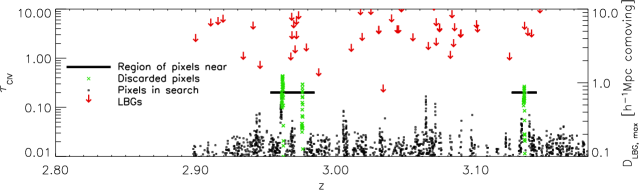
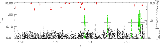
Figure 1: C IV pixel optical depth recovered from the spectrum of Q1422+231 is shown as a function of redshift (squares and crosses). The solid lines indicate regions corresponding to the near sample for $30~{}\mathrm{kms^{-1}}<|\Delta\upsilon|<600~{}\mathrm{kms^{-1}}$ and threshold optical depth $\tau_{\mathrm{C\scriptscriptstyle{IV},Thresh}}=0.2$. The solid lines are positioned vertically at the threshold in $\tau_{\mathrm{C\scriptscriptstyle{IV}}}$. Pixels that are discarded because they are within $30~{}{\rm km}\,{\rm s}^{-1}$ of marker pixels are shown as green crosses. Positions of LBGs near the line of sight are indicated with red arrows and their impact parameters can be read off from the $y$-axis on the right-hand side.

Pixels near to and far from LBGs are selected as follows. First, LBGs with impact parameter $b<D_{\mathrm{LBG,max}}$ relative to the line of sight are each used to define a marker pixel with redshift $z=z_{\rm LBG}$. Second, the full sample of pixels is separated into those with $|\Delta v|\equiv|z-z_{\rm LBG}|c/(1+z_{\rm LBG})<600~{}{\rm km}\,{\rm s}^{-1}$ and those with $|\Delta v|>600~{}{\rm km}\,{\rm s}^{-1}$. Our choice for the maximum velocity difference is motivated by the observation that interstellar absorption lines in the spectra of high-redshift LBGs are typically blueshifted by up to $600~{}{\rm km}\,{\rm s}^{-1}$ (e.g., Pettini et al. 2001; Adelberger et al. 2003). Such blueshifts are widely interpreted as a signature of large-scale outflows.

As an alternative to using the LBGs, we also use strong C IV absorption as a tracer of galaxies, motivated by the findings of Adelberger et al. (2003, 2005), who compared the absorption seen in a number of quasar spectra with the redshifts of LBGs at small angular separations. Adelberger et al. (2005) conclude that where LBGs are closer than $\mathrm{\sim 0.25~{}h^{-1}}$ Mpc comoving, the average C IV column density is $\sim 10^{14}~{}{\rm cm}^{-2}$. They also find that the galaxy-C IV cross correlation length increases with $N_{\rm CIV}$, becoming comparable to the LBG autocorrelation for $N_{\rm CIV}\gtrsim 10^{12.5}~{}{\rm cm}^{-2}$. We use the fact that a C IV Voigt profile line with line width $b$ has a central optical depth of

$$\tau_{c,{\rm CIV}}=0.44\left({N_{\rm CIV}\over 10^{13}\,{\rm cm}^{-2}}\right)\left({10~{}{\rm km}\,{\rm s}^{-1}\over b}\right),$$ (1)

where $b\approx 10~{}{\rm km}\,{\rm s}^{-1}$ is typical for C IV lines (e.g., Rauch et al. 1996). Hence absorbers with $\tau_{\mathrm{C\scriptscriptstyle{IV}}}>0.1$ should cluster to LBGs as LBGs cluster to each other, and absorbers with $\tau_{\mathrm{C\scriptscriptstyle{IV}}}\gg 1$ are expected to reside within $10^{2}$ kpc proper of a LBG.

As with the LBGs, we split the pixels into subsets according to their velocity relative to the nearest marker pixel. Marker pixels are in this case defined as those pixels with $\tau_{\mathrm{C\scriptscriptstyle{IV}}}>\tau_{\mathrm{C{\scriptscriptstyle IV},Thresh}}$. All pixels within $\pm 30~{}{\rm km}\,{\rm s}^{-1}$ of a marker pixel are discarded from the search in order to exclude the possibility that any differences between the two samples are trivial consequences of the search method. This would be the case if most of the C IV in the near sample of pixels arose from the absorption lines that contain the marker pixels. In §3.2 we will use simulations to show that excluding the nearest $\pm 30~{}{\rm km}\,{\rm s}^{-1}$ is sufficient for this purpose. Figure 1 shows the $\tau_{\mathrm{C\scriptscriptstyle{IV}}}$ of those pixels near, far and discarded where $\tau_{\mathrm{C{\scriptscriptstyle IV},Thresh}}=0.2$

Figure 2 shows the fractions of pixels that belong to the near sample when LBGs (left-hand panel) or strong C IV (right-hand panel) are used as markers. A lack of variation in the fractions of pixels with changing $D_{\mathrm{LBG,max}}$ or $\tau_{\mathrm{C{\scriptscriptstyle IV},Thresh}}$ reflects a lack of markers in that range. For example there are no markers in the range $0.5<\tau_{\mathrm{C{\scriptscriptstyle IV},Thresh}}<0.75$ and $2.2<D_{\mathrm{LBG,max}}<2.5\mathrm{h^{-1}Mpc}$.

Figure 2: Contour plots showing the fractions of pixel pairs in the spectrum of Q1422+231 that are within a velocity $|\Delta\upsilon|$ of marker pixels. Left: Marker pixels are defined as those pixels that have the same redshift as a LBG with impact parameter $b<D_{\mathrm{LBG,max}}$. Only pixels in the redshift range $2.898<z<3.25$ are considered. Right: Marker pixels are defined as pixels with recovered optical C IV optical depth $\tau_{\mathrm{C\scriptscriptstyle{IV}}}>\tau_{\mathrm{C{\scriptscriptstyle IV},Thresh}}$. Only pixels in the redshift range $2.898<z<3.552$ are considered.

3 Results

3.1 Near to and far from LBGs

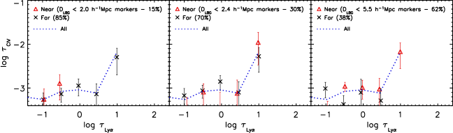
Figure 3: $\tau_{\mathrm{Ly\alpha}}$ - median apparent $\tau_{\mathrm{C\scriptscriptstyle{IV}}}$ relation for Q1422+231 derived using the two sample pixel correlation search for Civ. Redshifts of LBGs close to the line of sight (impact parameter $b<D_{\rm LBG}$) are used as markers for the separation of pixels into samples near to and far from observed galaxies. The maximum, comoving impact parameter used is 2.0, 2.4, and $5.5~{}h^{-1}\,{\rm Mpc}$ for the left, middle, and right panels respectively. The near sample (triangles) contains all pixels with $|\Delta v|<600~{}{\rm km}\,{\rm s}^{-1}$ from a marker redshift, while the far sample (crosses) is defined by $|\Delta v|>600~{}{\rm km}\,{\rm s}^{-1}$. The result for the full sample (dotted lines) of pixels is shown for comparison.

Figure 3 shows the results of the two sample search for C IV  when the redshifts of nearby LBGs are used as markers, and we divide our sample into the “near” pixels that are within $600~{}{\rm km}\,{\rm s}^{-1}$ of a marker redshift and the “far” pixels that are not. For each panel we take a different maximum LBG impact parameter $D_{\rm LBG,max}$.

In the left panel we use the lowest impact parameter that provides significant results for the near sample, $D_{\rm LBG,max}=2~{}h^{-1}\,{\rm Mpc}$ comoving (for smaller impact parameters the number of pixels and spectral regions in the near sample becomes too small to satisfy our statistical criteria). In the middle panel we use $D_{\rm LBG,max}=2.4~{}h^{-1}\,{\rm Mpc}$. This is the scale for which Adelberger et al. (2003) found that most of the C IV lines they detect are seen. In our case seven LBGs are within this distance from the line of sight. The right panel shows the case where $D_{\rm LBG,max}=5.5~{}h^{-1}\,{\rm Mpc}$ comoving. Such an impact parameter is chosen to represent the largest useful value for distance to LBGs since, at this redshift, this corresponds to $|\Delta v|\approx 600~{}{\rm km}\,{\rm s}^{-1}$ along the line of sight just due to the Hubble flow. There are no significant differences between the two samples for any of the choices of $D_{\rm LBG,max}$. This is also the case if we choose to disregard the non-uniform completeness and use the full redshift range up to $z=3.552$ .

This null result is somewhat surprising in light of the findings of Adelberger et al. (2003). However, we emphasize that our redshift path searched is very small ($\Delta z=0.352$) and that cosmic variance is therefore likely to be an issue. For example, it can be seen from Fig. 1 that our upper redshift cutoff of $z=3.25$ (above which the photometric selection of LBGs becomes highly incomplete) results in the exclusion of many of the stronger C IV absorbers in this spectrum, so that we do not have sufficient data to investigate the regime $\tau_{{\rm Ly}\alpha}>10$. It would thus clearly be desirable to repeat this analysis using the full sample of Adelberger et al. (2003, 2005). It should also be noted that our pixel technique is much more sensitive to weak C IV absorption than the method used by Adelberger et al. (2003) (i.e., direct detection by eye) and much of the absorption seen far from LBGs may be weak.

Perhaps the most natural explanation for our null result is that we are missing the vast majority of the galaxies from which the observed carbon originated. If metals were flowing out of galaxies at a constant velocity $v_{\rm wind}$, then they would reach a distance $1.0\times 10^{2}~{}{\rm kpc}\left({v_{\rm wind}\over 10^{2}~{}{\rm km}\,{\rm s}^{-1}}\right)\left({t\over 1{\rm Gyr}}\right)$ in a time $t$. Hence, it is natural to expect the sources of the observed intergalactic metals at $z=3$ to be located well within $1~{}h^{-1}\,{\rm Mpc}$ comoving of the line of sight. While we find a large number of C IV absorbers, there is only one galaxy that satisfies this criterion ($z\approx 3.03$, $b=33.66~{}{\rm arcsec}\approx 0.75~{}h^{-1}\,{\rm Mpc}$ comoving). This is perhaps not surprising, given the fact that only the bright end of the luminosity function is observable and that accurate redshifts can only be determined for a fraction of these bright galaxies. It does, however, illustrate the need for a tracer of galaxies that cannot be detected directly.

3.2 Near to and far from strong C IV

As discussed in §2, we have carried out a two-sample search for C IV and O VI absorption in regions near to and far from strong C IV absorbers. This approach was motivated by the work of Adelberger et al. (2003, 2005), who found that strong C IV is a good tracer of galaxies.

3.2.1 C IV

In Fig. 4 we plot the median, recovered C IV optical depth as a function of $\tau_{\rm HI}$ for pixels near (triangles) and far (crosses) from strong C IV absorbers. For comparison the results for the combined near and far samples (solid lines) and for the full sample of pixels (dotted lines) are also shown. Comparison with Fig. 3 shows that the near doubling of the redshift path searched ($\Delta z=0.654$ vs. $\Delta z=0.352$) significantly improves the statistics, particularly for high $\tau_{\rm HI}$.

The full sample and the combined near and far sample differ because only the full sample contains those pixels that are within $30~{}{\rm km}\,{\rm s}^{-1}$ of a marker pixel along with the marker pixel itself. As the threshold is lowered the results from these two samples become increasingly different as more pixels leave the combined near and far sample. The effect is pronounced for pixels with $\tau_{\rm HI}>10$ but is small for $\tau_{\rm HI}<10$. Since the systems of interest in this study are those with $\tau_{\rm HI}<10$ we can confirm that increasing the number of discarded pixels does not play a significant role.

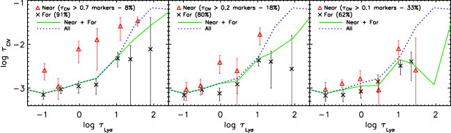
Figure 4: $\tau_{\mathrm{Ly\alpha}}$ - median apparent $\tau_{\mathrm{C\scriptscriptstyle{IV}}}$ relation for Q1422+231 derived using the two sample pixel correlation search for Civ. Strong Civ absorbers are used as markers for the separation of pixels into samples near to and far from relatively metal-rich regions. The threshold optical depth $\tau_{\mathrm{C\scriptscriptstyle{IV},Thresh}}$ is 0.7, 0.2 and 0.1 for the left, middle, and right panels respectively. The near sample (triangles) contains all pixels with $30~{}{\rm km}\,{\rm s}^{-1}<|\Delta v|<600~{}{\rm km}\,{\rm s}^{-1}$ from a marker redshift, while the far sample (crosses) is defined by $|\Delta v|>600~{}{\rm km}\,{\rm s}^{-1}$. The result for the combined (solid lines) and full (dotted lines) samples of pixels are shown for comparison.

The left, middle, and right panels use threshold optical depths, $\tau_{\mathrm{C{\scriptscriptstyle IV},Thresh}}$, of 0.7, 0.2, and 0.1, respectively, which covers the interesting range of values. Using $\tau_{\mathrm{C{\scriptscriptstyle IV},Thresh}}>0.7$, would leave only the lowest H I bins in the near sample with a sufficient number of pixels to satisfy our statistical criteria. The lower limit, $\tau_{\mathrm{C{\scriptscriptstyle IV},Thresh}}=0.1$, corresponds to the lowest optical depth which we can unambiguously identify as being due to C IV, and also corresponds to the central optical depth above which C IV absorption lines cluster to LBGs as LBGs cluster to each other (see §2). In addition, the number of pixels with $\tau_{{\rm Ly}\alpha}\gg 1$ becomes insufficient for $\tau_{\mathrm{C{\scriptscriptstyle IV},Thresh}}<0.1$ because in that case many pixels fall within $30~{}{\rm km}\,{\rm s}^{-1}$ of a marker pixel.

In each panel the near sample consists of all pixels that are at most $600~{}{\rm km}\,{\rm s}^{-1}$ from the nearest marker pixel, which are defined by $\tau>\tau_{\mathrm{C{\scriptscriptstyle IV},Thresh}}$, and at least $30~{}{\rm km}\,{\rm s}^{-1}$ from all marker pixels. The far sample always consists of the pixels that are at least $600~{}{\rm km}\,{\rm s}^{-1}$ from all marker pixels. The fractions of pixels contained in the near and far samples are indicated in the panels, the fractions do not sum to exactly 100% because the combined sample still excludes those pixels that are within $30~{}{\rm km}\,{\rm s}^{-1}$ of a marker pixel.

It is clear that, for fixed $\tau_{\rm HI}$, the C IV absorption is much stronger for pixels in the vicinity of $\tau_{\mathrm{C\scriptscriptstyle{IV}}}>0.7$ and 0.2 absorbers than for pixels that are at least $600~{}{\rm km}\,{\rm s}^{-1}$ away from such marker pixels. Since $[{\rm C}/{\rm H}]\propto\log\tau_{\mathrm{C\scriptscriptstyle{IV}}}$ for fixed $\tau_{\rm HI}$ if the gas if photoionized, we see that in these regions carbon may be overabundant by up to an order of magnitude compared to the global median. However, when we lower the threshold optical depth from $\tau_{\mathrm{C\scriptscriptstyle{IV}}}=0.2$ to 0.1, and thus increase the fraction of pixels in the near sample from 18 to 33 percent, the differences between the samples become insignificant. These results show that the H I optical depth, which is thought to be a good indicator of the gas density, is not the only parameter that correlates with metal enrichment. Proximity to highly enriched regions and (by extension) galaxies clearly also plays an important role.

Interestingly, the results for the far sample are always consistent with those for the combined samples and disagree with the full sample only for the highest H I bins ($\tau_{\rm HI}\gg 10$), where the full sample becomes dominated by pixels within $30~{}{\rm km}\,{\rm s}^{-1}$ of a $\tau_{\mathrm{C\scriptscriptstyle{IV}}}>0.1$ marker pixel. The median apparent $\tau_{\mathrm{C\scriptscriptstyle{IV}}}$ is always substantially higher for $\tau_{\rm HI}\gtrsim 10$ than for $\tau_{\rm HI}\ll 10$, even if we only consider the 62% of the pixels that are at least $600~{}{\rm km}\,{\rm s}^{-1}$ from any pixels that have $\tau_{\mathrm{C\scriptscriptstyle{IV}}}>0.1$ (crosses in the right-hand panel). Thus, it appears that carbon enrichment is not confined to the immediate surroundings of highly enriched regions.

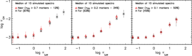
Figure 5: $\tau_{\mathrm{Ly\alpha}}$ - median apparent $\tau_{\mathrm{C\scriptscriptstyle{IV}}}$ relation for 10 simulated spectra derived using the two sample pixel correlation search for Civ as used in Fig. 4. Data points indicate the medians of the 10 spectra. The synthetic spectra were taken from a cosmological, hydrodynamical simulation in which the metals are distributed according to the measurements of Schaye et al. (2003). The metal distribution is stochastic and depends only on the gas density and redshift.

At this point some scepticism would certainly be justified. Since we are looking for C IV in regions selected by C IV, aren’t our results a trivial consequence of the search method? Figure 5 demonstrates that is not the case. The figure is identical to Fig. 4, except that we have now plotted the results for spectra drawn from a cosmological, hydrodynamical simulation in which the metals were distributed according to the observations of Schaye et al. (2003), who measured the distribution of carbon (including the scatter) as a function of density and redshift, as inferred from C IV absorption in a large set of quasar spectra. The simulation, the procedures for creating a spectrum that mimics the observations, and the metal distribution are all described in detail in Schaye et al. (2003); for present purposes the key point is that the metallicity assigned to the gas depends on the gas density but not explicitly on the gas’s proximity to galaxies. Clearly, splitting the pixels into samples near to and far from strong C IV absorbers has no effect for these synthetic spectra. This demonstrates that the significant differences between the two observed samples cannot be explained as an artifact of the search method.

It was shown by Schaye et al. (2003) that, for fixed $\tau_{\rm HI}$, the $\tau_{\mathrm{C\scriptscriptstyle{IV}}}$ distribution in Q1422+231 is well-fit by a lognormal distribution of width $\sigma(\log\tau_{\mathrm{C\scriptscriptstyle{IV}}})=\sigma([{\rm C}/{\rm H}])\simeq 0.8$. Now that we have established that proximity to highly enriched gas is a second parameter, along with density, that controls the amount of C IV absorption, it is interesting to ask whether this parameter is responsible for the large amount of scatter in $\tau_{\mathrm{C\scriptscriptstyle{IV}}}$ for fixed $\tau_{\rm HI}$. To test this, we have determined $\sigma(\log\tau_{\mathrm{C\scriptscriptstyle{IV}}})$ near to and far from strong C IV absorbers.

Briefly, the method used is as follows (see Schaye et al. 2003 for more detail). For each $\tau_{{\rm Ly}\alpha}$ bin, we calculate many percentiles $\log\tau_{\mathrm{C\scriptscriptstyle{IV}}}(s)$, where $s$ is the number of standard deviations in a Gaussian distribution; for example, $\log\tau_{\mathrm{C\scriptscriptstyle{IV}}}(s=0)$ and $\log\tau_{\mathrm{C\scriptscriptstyle{IV}}}(s=1)$ would, respectively, correspond to the 50th and 84th percentiles in the $\log\tau_{\mathrm{C\scriptscriptstyle{IV}}}$ distribution. Errors on these points are calculated using the same bootstrap procedure as described in §2. From each of these, we subtract $\log\tau_{\rm CIV}(s)$ computed from all pixels (in the full undivided sample) with $\tau_{{\rm Ly}\alpha}<-0.5$; in this way, we subtract off the effect of noise and contamination that is uncorrelated with $\tau_{{\rm Ly}\alpha}$. Next, we fit a line to the function $\log\tau_{\mathrm{C\scriptscriptstyle{IV}}}(s)$, which corresponds to a lognormal fit to the $\tau_{\mathrm{C\scriptscriptstyle{IV}}}$ probability distribution; the slope of the linear fit to $\log\tau_{\mathrm{C\scriptscriptstyle{IV}}}(s)$ is the width $\sigma(\log\tau_{\rm CIV})$ of the lognormal distribution, in dex. To obtain errors we repeat the procedure using bootstrap-resampled realizations of the spectrum.

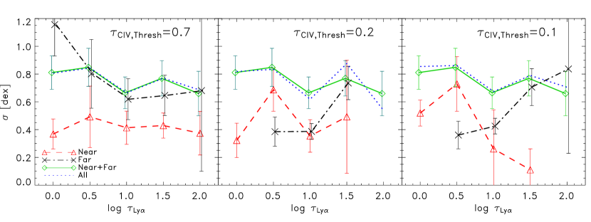
Figure 6: Scatter in the C IV abundance for various samples of pixels. Each point corresponds to the scatter $\sigma$ in $\log\tau_{\mathrm{C\scriptscriptstyle{IV}}}$, in dex, for a bin of $\log\tau_{{\rm Ly}\alpha}$. The samples are identical to those in Fig. 4.

The results are shown in Figure 6 for the threshold C IV optical depths 0.7 (left), 0.2 (middle), and 0.1 (right). In all cases there is significantly less scatter in the near sample than in the full sample. In addition, for $\tau_{\mathrm{C{\scriptscriptstyle IV},Thresh}}=0.2$ and 0.1, there is some evidence that the scatter in the far sample is also smaller. These results suggest that variations in the distance to the nearest galaxy is responsible for a substantial fraction of the scatter in the metallicity of gas at a fixed density.

3.2.2 O VI

The strong Civ markers can of course also be used in searches for other ions. Figure 7 shows the results for O VI. The redshift range searched, the threshold C IV optical depths, and velocity range are all the same as in the C IV search. The small differences in the fractions of pixels belonging to the various samples between Figs 4 and 7 are due to differences between the numbers of O VI and C IV pixels discarded due to noise spikes, sky lines, and contamination.

As was the case for C IV, there are significant differences between the near and far samples for $\tau_{\rm CIV,Thresh}=0.7$ and 0.2, although the differences are much smaller than was the case for C IV ($\sim 0.5$ dex rather than 1 dex). In contrast to C IV, we find no evidence for O VI absorption in any of the far samples, except perhaps tentatively in the very highest H I bin ($\tau_{\rm HI}\sim 10^{2}$). These results indicate that either oxygen enrichment is less widespread than carbon, or that away from the highly enriched regions oxygen is too weak to detect. The latter scenario appears more plausible and would also explain why the samples differ less in $\tau_{\rm OVI}$ than in $\tau_{\mathrm{C\scriptscriptstyle{IV}}}$ (even if the difference in the true, median $\tau_{\rm OVI}$ between the near and far samples were as large as a factor ten, we would not be able to tell if the median for the near sample is only $\sim 0.5$ dex above the detection limit).

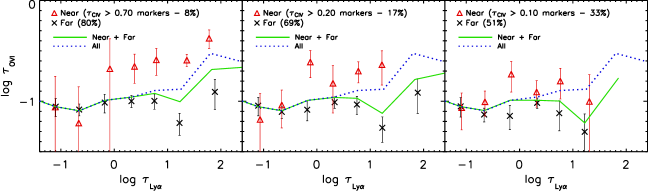
Figure 7: As Fig. 4, except that we search for Ovi instead of Civ. The pixels are, however, still divided into samples near to and far from strong Civ

.

It would be interesting to repeat this analysis at $z\sim 2.5$, where the pixel search has been shown to be able to produce a strong O VI signal (Schaye et al., 2000). Aracil et al. (2004) have in fact performed a two-sample pixel search for O VI at this redshift, but using strong H I absorbers as markers rather than strong C IV. They found that for $\log\tau_{\rm HI}\approx-0.5$ the corresponding O VI is only detectable in the near sample, which in their case consisted of all pixels that are less than $500~{}{\rm km}\,{\rm s}^{-1}$ from a pixel with $\tau_{\rm HI}>4$ (they do not give the fraction of pixels represented by this subset, but we note that for Q1422+231 their choice of parameters would put 88% of the pixels in the near sample).

4 Conclusions

We have searched for absorption by C IV and O VI absorption at $2.898\leq z\leq 3.552$ in a high-quality spectrum of quasar Q1422+231. We can summarize our findings regarding the spatial distribution of metal enrichment in the intergalactic medium as follows:

• No correlations between metal line absorption and the positions of Lyman-break galaxies are found. This may not be inconsistent with findings by others based on substantially larger samples which focused on stronger C IV absorbers. This part of our analysis was restricted to the redshift range $2.898<z<3.25$ - a comparatively narrow range required by the need for consistent completeness in the detection of LBGs.

• We find a strong correlation between metal line absorption and the location of strong C IV absorbers, which Adelberger et al. (2003, 2005) found to be good tracers of galaxies. Two-sample searches for C IV and O VI near and far from strong C IV absorbers demonstrate that the enrichment depends not only on the density, but also on the proximity to regions that are highly enriched (and so proximity to galaxies).

• The variations in proximity to highly enriched regions can account for a substantial part of the scatter in the abundance of carbon for a fixed H I strength.

• In searching for weak C IV it is clear that the enrichment is much more widespread than the regions surrounding strong metal-line absorption, but for O VI the detection limit (which is set by contamination from the H I Lyman series) is too high to probe the enrichment in all but the most metal rich regions.

• Metal enrichment is seen both far from currently detectable galaxies and far from strong C IV absorbers.

References

- Adelberger et al. (2003) Adelberger, K. L., Steidel, C. C., Shapley, A. E., & Pettini, M. 2003, ApJ, 584, 45
- Adelberger et al. (2005) Adelberger, K. L., Shapley, A. E., Steidel, C. C., Pettini, M., Erb, D. K., Reddy, N. A. 2005, ApJ, in press (astro-ph/0505122)
- Aguirre et al. (2004) Aguirre, A., Schaye, J., Kim, T., Theuns, T., Rauch, M., & Sargent, W. L. W. 2004, ApJ, 602, 38
- Aguirre et al. (2002) Aguirre, A., Schaye, J., & Theuns, T. 2002, ApJ, 576, 1
- Aracil et al. (2004) Aracil, B., Petitjean, P., Pichon, C., & Bergeron, J. 2004, A&A, 419, 811
- Bahcall & Spitzer (1969) Bahcall, J. N., & Spitzer, L. J. 1969, ApJ, 156, L63
- Barlow & Sargent (1997) Barlow, T. A., & Sargent, W. L. W. 1997, AJ, 113, 136
- Bergeron & Boisse (1991) Bergeron, J., & Boisse, P. 1991, A&A, 243, 344
- Bergeron et al. (2002) Bergeron, J., Aracil, B., Petitjean, P., & Pichon, C. 2002, A&A, 396, L11
- Carswell et al. (2002) Carswell, B., Schaye, J., & Kim, T. 2002, ApJ, 578, 43
- Chen et al. (2001) Chen, H., Lanzetta, K. M., & Webb, J. K. 2001, ApJ, 556, 158
- Cowie et al. (1995) Cowie, L. L., Songaila, A., Kim, T., & Hu, E. M. 1995, AJ, 109, 1522
- Cowie & Songaila (1998) Cowie, L. L., & Songaila, A. 1998, Nat, 394, 44
- Haehnelt et al. (1996) Haehnelt, M. G., Steinmetz, M., & Rauch, M. 1996, ApJ, 465, L95
- Hellsten et al. (1997) Hellsten, U., Dave, R., Hernquist, L., Weinberg, D. H., & Katz, N. 1997, ApJ, 487, 482
- Mori et al. (2002) Mori, M., Ferrara, A., & Madau, P. 2002, ApJ, 571, 40
- Pettini et al. (2001) Pettini, M., Shapley, A. E., Steidel, C. C., Cuby, J., Dickinson, M., Moorwood, A. F. M., Adelberger, K. L., & Giavalisco, M. 2001, ApJ, 554, 981
- Pieri & Haehnelt (2004) Pieri, M. M., & Haehnelt, M. G. 2004, MNRAS, 347, 985
- Rauch et al. (1996) Rauch, M., Sargent, W. L. W., Womble, D. S., Barlow, T. A. 1996, ApJ, 467,L5,
- Scannapieco et al. (2005) Scannapieco, E., Pichon, C., Aracil, B., Petitjean, P., Thacker, R. J., Pogosyan, D., Bergeron, J., & Couchman, H. M. P. 2005, MNRAS, submitted (astro-ph/0503001)
- Schaye et al. (2000) Schaye, J., Rauch, M., Sargent, W. L. W., & Kim, T. 2000, ApJ, 541, L1
- Schaye et al. (2003) Schaye, J., Aguirre, A., Kim, T., Theuns, T., Rauch, M., & Sargent, W. L. W. 2003, ApJ, 596, 768
- Simcoe et al. (2004) Simcoe, R. A., Sargent, W. L. W., & Rauch, M. 2004, ApJ, 606, 92
- Songaila (2001) Songaila, A. 2001, ApJL, 561, L153
- Steidel et al. (2003) Steidel, C. C., Adelberger, K. L., Shapley, A. E., Pettini, M., Dickinson, M., & Giavalisco, M. 2003, ApJ, 592, 728
- Vogt et al. (1994) Vogt, S. S., et al. 1994, Proc. SPIE, 2198, 362