Morphological Classification of Galaxies
using Photometric Parameters: the Concentration index versus the Coarseness parameter

Abstract

We devise improved photometric parameters for the morphological classification of galaxies using a bright sample from the First Data Release of the Sloan Digital Sky Survey. In addition to using an elliptical aperture concentration index for classification, we introduce a new texture parameter, coarseness, which quantifies deviations from smooth galaxy isophotes. The elliptical aperture concentration index produces morphological classifications that are in appreciably better agreement with visual classifications than those based on circular apertures. With the addition of the coarseness parameter, the success rate of classifying galaxies into early and late types increases to $\simeq 88$% with respect to the reference visual classification. A reasonably high success rate ($\simeq 68$%) is also attained in classifying galaxies into three types, early-type galaxies (E+S0), early- (Sa+Sb) and late- (Sc+Sdm+Im) type spiral galaxies.

1 Introduction

The morphological classification of galaxies, which assigns galaxies discrete classes in the form of a tuning-fork diagram (the so called Hubble sequence, Sandage 1961), allows us to quantify the basic features of galaxies and to relate them to the galaxies’ formation and evolution histories. While the Hubble classification is based on the visual inspection of images of galaxies, and therefore necessarily involves subjective elements, it provides a basis for many extragalactic studies (e.g., Dressler 1980; Binggeli, Sandage & Tammann 1988; Dressler 1994).

With the advancement of digitized galaxy surveys, it is highly desirable to develop a fast, automated method of morphological classification applicable to large data samples, without loosing the accuracy of the traditional visual classification. The typical approaches employed for morphological classification are to apply artificial neural networks (Burda & Feitzinger, 1992; Storrie-Lombardi et al., 1992; Serra-Ricart et al., 1993; Naim et al., 1995; Odewahn et al., 2002; Ball et al., 2004), and characterizations with simple surface photometric parameters (Doi, Fukugita & Okamura, 1993; Abraham et al., 1994). In this paper, we focus on the photometric parameters for the morphological classification of galaxies using Sloan Digital Sky Survey (SDSS, York et al. 2000; Early Data Release, Stoughton et al. 2002, hereafter EDR; First Data Release, Abazajian et al. 2003, hereafter DR1; Second Data Release, Abazajian et al. 2004) imaging data. The simplest indicator often used in the literature is the parameter that characterizes the concentration of light towards the center of galaxies (Morgan, 1958). Doi et al. (1993) defined the concentration index⁾ using two equivalent radii of the elliptic isophotes. They show that early- and late-type galaxies are reasonably well separated in isophotal photometry, if surface brightness is used as a second parameter. Abraham et al. (1996) introduced a rotational asymmetry parameter $A$ in addition to $C$ that is defined using the flux measured in elliptical apertures. The rotational asymmetry parameter allows for efficient discrimination between irregular and spiral galaxies. The $\log C$-$\log A$ diagram has been used as a tool to classify morphology of distant galaxies observed with the HST (e.g., Abraham et al. 1996; Brinchmann et al. 1998). Takamiya (1999) discusses the evolution of the structure of galaxies using $\chi$ parameter calculated from the residual image, which indicates the power at high spatial frequencies in the disk of the galaxy. Shimasaku et al. (2001) and Strateva et al. (2001) showed that the concentration index, calculated using circular isophotes as part of the standard SDSS pipeline reductions (Stoughton et al. 2002), correlates fairly well with morphological type and can be used for classification into early and late galaxy types. The success rate of these approaches, with reference to visual inspection, is approximately $80$%.

In this paper, we use the SDSS Data Release 1 (DR1, Abazajian et al. 2004) imaging data of 1421 galaxies selected from the SDSS Early Data Release (EDR, Sthoughton et al. 2002) and early commissioning data to improve the success rate of morphological classifiers by introducing additional photometric parameters. First, we consider the performance of the standard circular-aperture concentration index, with particular emphasis on the cases where the classification fails. We proceed to employ the elliptical definition of Doi et al. (1993) and Abraham et al. (1996) for the measurement of isophotal and aperture fluxes and compare the success rate to that obtained using the circular definition. We also introduce a new texture parameter to help our classification. The motivation for this approach is that, in the visual classification, we mainly resort to surface brightness texture, such as properties of spiral arms, clumpiness, and HII regions, in addition to the concentration of light towards the galaxy center. The only work that we are aware of that discusses texture parameters as a classifier is that by Naim, Ratnatunga & Griffiths (1997). They proposed “blobbiness”, “isophotal center displacement” and “skeleton ratio” parameters, which correspond to roughness, global asymmetries and more localized structure, respectively. These parameters correlate with galaxy morphology and may be useful for classification, but our own tests show that they do not enhance the success rate of the classifier. Our texture parameter – coarseness – describes the structure of the outer galaxy isophotes, emulating the method employed in visual classification. The flux fluctuations are computed along elliptical circumferences in order to characterize the galaxy profile’s departure from smoothness. The coarseness parameter is defined as the ratio of the range of fluctuations in surface brightness along the elliptic circumference to the full dynamic range of surface brightness of the galaxy. In this study we evaluate the performance of the elliptical concentration index and the coarseness parameter as classification parameters (used separately or together) in comparison to the visually classified SDSS sample of Fukugita et al. (in preparation).

This paper is organized as follows. The elliptical-aperture concentration index is defined in section 2. The coarseness parameter is introduced in section 3. After briefly describing our sample in section 4, the correlation of the two parameters with the visually obtained morphology is investigated in section 5. We study the performance of the morphological classification using these parameters in section 6, and conclusions are presented in section 7.

2 CONCENTRATION INDEX

We consider a concentration index for elliptical apertures using Petrosian quantities. The intensity-weighted second-order moments are defined in the SDSS photometric pipeline (hereafter PHOTO; Lupton 1996; Lupton et al. 2001) as

$$M_{xx}\equiv\langle x^{2}/r^{2}\rangle,~{}M_{xy}\equiv\langle xy/r^{2}\rangle,~{}M_{yy}\equiv\langle y^{2}/r^{2}\rangle.$$ (1)

If the major and minor axes of the ellipse lie along the $x$ and $y$ axes, the axis ratio $\alpha=b/a$ is calculated as

$$\alpha=\frac{M_{yy}}{M_{xx}}.$$ (2)

because

$$M_{xx}=\frac{1}{1+\alpha},~{}~{}~{}~{}M_{xy}=0,~{}~{}~{}~{}M_{yy}=\frac{\alpha}{1+\alpha}.$$ (3)

In general, we rotate the image to account for the position angle $\phi$ from $(x^{\prime},y^{\prime})$ to $(x,y)$ to align the galaxy image along the axes:

$${x^{\prime}=x\cos\phi-y\sin\phi\atop y^{\prime}=x\sin\phi+y\cos\phi.}$$ (4)

The Stokes parameters $U$ and $Q$ are calculated as

$$U/2\equiv M_{x^{\prime}y^{\prime}} = (M_{xx}-M_{yy})\sin\phi\cos\phi$$ (5)

$$= \frac{1-\alpha}{1+\alpha}\cdot\frac{\sin 2\phi}{2}$$

$$Q\equiv M_{x^{\prime}x^{\prime}}-M_{y^{\prime}y^{\prime}}=\frac{1-\alpha}{1+\alpha}\cos 2\phi,$$ (6)

where $\phi=1/2~{}{\rm tan}^{-1}(U/Q)$. The axis ratio is $\alpha=(1+P)/(1-P)$ with $P=\sqrt{(U^{2}+Q^{2})}$. $U$ and $Q$ are evaluated in PHOTO and cataloged in the SDSS data releases.

To calculate the concentration index $C_{e}$ for the ellipse, we consider the area $A_{e}(a)$ of the ellipse of the semi-major axis $a$ and axis ratio $\alpha$, and the integrated flux $F_{e}(a)$ within $A_{e}(a)$. We define the Petrosian semi-major axis $a_{\rm P}$ for a given $\eta$ as

$$\scriptsize\eta=\frac{\{F_{e}(1.25a_{\rm P})-F_{e}(0.8a_{\rm P})\}/\{A_{e}(1.25a_{\rm P})-A_{e}(0.8a_{\rm P})\}}{F_{e}(a_{\rm P})/A_{e}(a_{\rm P})},$$ (7)

where we take $\eta$=$0.2$, and the elliptical Petrosian flux $F_{\rm P}$ as

$$F_{\rm P}=F_{e}(ka_{\rm P})$$ (8)

with $k$ set equal to 2, following the SDSS definition (Strauss et al., 2002).

The Petrosian half-light and 90%-light semi-major axes $a_{\rm 50}$, $a_{\rm 90}$ are defined in such a way that the flux in the elliptical apertures of these semi-major axes is 50% and 90% of the elliptical Petrosian flux:

$$F_{e}(a_{50})=0.5F_{\rm P},~{}~{}F_{e}(a_{90})=0.9F_{\rm P}~{}.$$ (9)

We define our concentration index $C_{e}$ by

$$C_{e}=a_{\rm 50}/a_{\rm 90}~{}.$$ (10)

3 THE COARSENESS PARAMETER

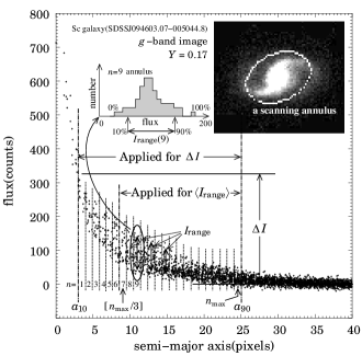
Figure 1: An illustration explaining the method of computing $Y$ for the galaxy image inlaid in the top right of the figure. The figure shows division of the area sandwiched by the two ellipses specified by $a_{90}$ and $a_{10}$ into $n_{\rm max}$ annuli. The dotted lines show division into elliptical annuli. The range of flux $I_{\rm range}(n)$ is defined by the 90%- and 10%-tiles of the flux distribution of $n$-th annulus as an inlaid histogram in the top left of the figure. The $I_{\rm range}$ computed in each annulus is averaged over $N$ annuli to give $\langle I_{\rm range}\rangle$, and the coarseness parameter $Y$ is given as $\langle I_{\rm range}\rangle$ divided by the full dynamic range of the flux observed for the galaxy, $\Delta I$.

3.1 Definition of a Texture Parameter

In this section we provide a detailed “step-by-step” method for the calculation of the coarseness parameter. The position angle $\phi$ and the axis ratio $\alpha$ are calculated in the same way as in the previous section. Each position $(x,y)$ of pixel on the image is calculated by equation (4) beforehand, so that the semimajor and semiminor axes are aligned with the $x$ and $y$ axis.

We consider successive elliptical annuli from $a=a_{\rm 10}$ outwards to $a_{\rm 90}$, where $a_{f}$ is defined by $F_{e}(a_{f})=\frac{f}{100}F_{\rm P}$ as in equation (9), assuming that each elliptical annulus has the same position angle and is congruent. We define the ‘equivalent distance’ $d$ from the center of the galaxy to a pixel at $(x,y)$ by

$$d=\sqrt{x^{2}+(y/\alpha)^{2}}.$$ (11)

We then divide the area sandwiched by the two ellipses specified by $a_{\rm 10}$ and $a_{\rm 90}$ into $n_{\rm max}$ annuli, as specified in what follows: We calculate $d$ of each pixel contained in the annulus between $a_{\rm 10}$ and $a_{\rm 90}$, and place the pixels in ascending order with respect to $d$ as

$$\scriptsize\underbrace{d_{1_{1}},d_{1_{2}},\cdot\cdot\cdot,d_{1_{{\cal N}_{1}}}},~{}\underbrace{d_{2_{1}},d_{2_{2}},\cdot\cdot\cdot,d_{2_{{\cal N}_{2}}}},~{}\underbrace{d_{3_{1}},d_{3_{2}},\cdot\cdot\cdot,d_{3_{{\cal N}_{3}}}},~{}\cdot\cdot\cdot~{},~{}\atop{\rm 1st~{}annulus~{}~{}~{}~{}~{}~{}~{}~{}~{}~{}2nd~{}annulus~{}~{}~{}~{}~{}~{}~{}~{}~{}~{}3rd~{}annulus}~{}~{}\cdot\cdot\cdot~{}~{}~{}~{}$$ (12)

where the number of pixels contained in the $n$-th annulus ${\cal N}_{n}$ is calculated by the equivalent distance to the innermost point in the $n$-th annulus, $d_{n_{1}}$:

$${\cal N}_{n}=[2\pi\alpha d_{n_{1}}]~{},$$ (13)

where $[x]$ is the integer part of $x$. The last annulus, which terminates at $a_{90}$, does not generally satisfy the condition (13). We show the actual algorithm which satisfies equation (12) and (13) as follows:

1) Focus on 1st $d$, $d_{1_{1}}$.

2) Calculate ${\cal N}_{1}$ by equation (13), ${\cal N}_{1}=[2\pi\alpha d_{1_{1}}]$.

3) When ${\cal N}_{1}$=6 for an example⁾, the member of 1st annulus is

$$d_{1_{1}},d_{1_{2}},d_{1_{3}},d_{1_{4}},d_{1_{5}}~{}{\rm and}~{}d_{1_{6}}.$$

4) $d_{2_{1}}$ is automatically determined by $d_{1_{6}}$ ($d_{2_{1}}$ is next to $d_{1_{6}}$. That is, 7th $d$).

5) Focus on 7th $d$, $d_{2_{1}}$.

6) Calculate ${\cal N}_{2}$ by equation (13), ${\cal N}_{2}=[2\pi\alpha d_{2_{1}}]$ $\cdot\cdot\cdot$

Let us take the $n$-th annulus, and consider the flux distribution. We denote the 90%- and 10%-tiles of the flux distribution in the $n$-th annulus as $I_{90}(n)$ and $I_{10}(n)$, respectively (see the inlaid histogram in the top left of Figure 1), and the range of the two values as

$$I_{\rm range}(n)=I_{90}(n)-I_{10}(n)~{}.$$ (14)

We define the mean of $I_{\rm range}(n)$ over the annuli between $n_{\rm begin}$ and $n_{\rm max}$, as

$$\langle I_{\rm range}\rangle=\frac{1}{n_{\rm max}-(n_{\rm begin}-1)}\sum_{n=n_{\rm begin}}^{n_{\rm max}}I_{\rm range}(n),$$ (15)

where the mean is taken from the $n_{\rm begin}$-th to the outermost annulus, some inner annuli being excluded. The exclusion of the inner radius is necessary in order to enhance the visibility of texture, which is usually more pronounced in outer regions for late-type galaxies. From trial and error, we adopted $n_{\rm begin}=[n_{\rm max}/3]$ with the floor function as the best value for the performance of classification.

To further enhance the signal, we subtract the contribution of the sky noise from $\langle I_{\rm range}\rangle$,

$$I_{\rm signal}=\sqrt{\langle I_{\rm range}\rangle^{2}-(2.56\cdot\varsigma_{\rm sky})^{2}}\ ,$$ (16)

where $\varsigma_{\rm sky}$ denotes the rms of the sky noise. We multiply the sky noise by a factor of 2.56 so that its strength corresponds to the range between 90 and 10%-tiles in the Gaussian distribution to match our definition of $I_{\rm range}$. With this choice, $I_{\rm signal}$ vanishes when the frame does not contain objects, i.e., contains sky noise only.

We then divide $I_{\rm signal}$ by the dynamic range of the image $\Delta I$, i.e.,

$$Y=\frac{I_{\rm signal}}{\Delta I}~{}.$$ (17)

The $\Delta I$ is defined by

$$\Delta I={\rm max}\{I_{90}(n)\}-{\rm min}\{I_{10}(n)\}~{},$$ (18)

where ${\rm max}\{\}$ and ${\rm min}\{\}$ are taken from $1\leq n\leq n_{\rm max}$. We use all annuli in the computation of $\Delta I$, not just $n_{\rm begin}\leq n\leq n_{\rm max}$, which allows us to increase the signal contrast.

This procedure is sketched in Figure 1, which shows the flux of each pixel of a test image plotted as a function of its semi-major axis. Note that, in the absence of noise, the $Y$ parameter vanishes if the profile is a smooth function (such as a model de Vaucouleurs or a model exponential profile), since this corresponds to $I_{\rm range}=0$. On the other hand, if structures such as spiral arms are present, both $I_{\rm range}$ and $Y$ become non-zero.

3.2 Image Rescaling

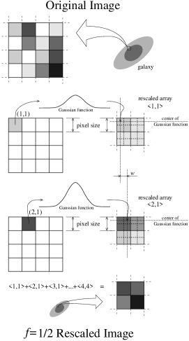
Figure 2: The method of creating rescaled images ($f=1/2$). Each Gaussian function whose intensity is $I(x,y)\cdot f^{2}$ and width is adjusted to the effective seeing will be mapped to the rescaled array. The mapping $<$1,1$>$+$<$2,1$>$+…+$<$4,4$>$ which creates the rescaled image conserves the surface brightness.

The coarseness parameter thus defined may depend on the apparent size of galaxies, because larger images are resolved in finer details. To avoid this dependence, we set the reference size of the galaxy image, and reduce the size of larger galaxies to the reference size. The coarseness parameter is measured for the rescaled image. The number of pixels in the rescaled image is taken to be that in the reference image. The reduction of image size takes into account both the fact that the rescaling factor is generally non-integer and the image variations in seeing, as explained below and illustrated in Figure 2. We exclude from further consideration galaxies with apparent sizes smaller than our chosen reference size.

We rescale the image with the semimajor axis $a_{\rm 90}$ to the reference size image with $a_{\rm 90}^{\rm ref}$ using Gaussian functions. We assign a Gaussian function to each pixel and map it to the rescaled array. The Gaussian function for the pixel at $(x,y)$ is constructed so that its integral equals $I(x,y)f^{2}$, with the rescaling factor, $f$, given by:

$$f=\frac{a_{90}^{\rm ref}}{a_{90}}~{}.$$ (19)

The Gaussian width $\sigma_{xy}$ is

$$\sigma_{xy}=\sqrt{\sigma_{\rm ref}^{2}-(\sigma_{\rm seeing}f)^{2}}~{}.$$ (20)

where $\sigma_{\rm ref}$ is the seeing taken as our reference and $\sigma_{\rm seeing}$ is the actual seeing of each image. With this procedure the PSF in the rescaled image is standardized by varying $\sigma_{xy}$ from image to image. The Gaussian functions with $\sigma_{xy}$ are projected onto a new array with the interval of pixels

$$w=f\times{\rm pixel~{}size}~{}.$$ (21)

This projection conserves surface brightness.

Figure 3: Effective ratio of sky noise $f_{s}$ for the rescaled image as a function of the scaling factor $f$ for a given seeing $\sigma_{xy}$.

The use of rescaled images requires similar adjustment of the observed sky noise $\varsigma$:

$$\varsigma_{\rm sky}=f_{s}\cdot\varsigma,$$ (22)

where $f_{s}$ is the effective ratio of standard deviation obtained from an artificial sky-noise image to which equivalent Gaussian smearing has been applied. The quantity $f_{s}$, shown in Figure 3, depends on both $\sigma_{xy}$ and the pixel size.

		Total Sample		Our Sample
Hubble Type	$T$	Number	Percent	Number	Ratio
unclassified	$-$1	23	1.3%	—	—
E	0	242	13.3%	194	13.7%
S0	0.5, 1	494	27.2%	343	24.1%
Sa	1.5, 2	309	17.0%	211	14.8%
Sb	2.5, 3	301	16.6%	250	17.6%
Sc	3.5, 4	337	18.5%	314	22.1%
Sdm	4.5, 5	80	4.4%	80	5.6%
Im	5.5, 6	31	1.7%	29	2.0%
Total		1817	100%	1421	100%

Table 1: Morphological compositions of the total sample and the sample after applying the size cutoff and dropping $T$=$-1$ class.

4 THE SAMPLE

The galaxies used in our test are taken from the northern equatorial stripe given in SDSS DR1 (Abazajian et al., 2003). The photometric system, imaging hardware and astrometric calibration of SDSS are described in detail elsewhere (Fukugita et al., 1996; Gunn et al., 1998; Hogg et al., 2001; Smith et al., 2002; Pier et al., 2003). We use the catalog of visual morphological classification provided by Fukugita et al. (in preparation; see also Nakamura et al. 2003) based on the $g$-band image. This catalog is based on the SDSS-EDR and early commissioning data, and contains 1875 galaxies brighter than $r^{*}$=$15.9$, where $r^{*}$ is the extinction corrected Petrosian magnitude ⁾. Using positional matching we identify galaxies in the Fukugita et al. catalog with DR1 objects. This allows us to weed out “fake” galaxies present in the catalog as a result of erroneous galaxy deblends in the EDR and early commissioning data. This positional matching reduces the number of galaxies in the Fukugita et al. catalog by 58, and then the number of the total sample is reduced to 1817 galaxies. The galaxies are classified into $T$=$-1$ as unclassified and 13 morphological types from $T$=$0$ (corresponding to E in the Hubble type) to $6$ (Im) allowing for half integer classes. In this paper, we mostly refer to $T$=0 as E, 0.5 and 1 as S0, 1.5 and 2 as Sa, …, 5.5 and 6 as Im, as designated in Table 1, where the number of galaxies in each class is shown.

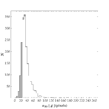
Figure 4: Distribution of the semi-major axes containing 90% of the Petrosian flux of the 1817 galaxies in the SDSS $g$-band (1 pixel = 0.4 arcsec). The shaded region indicates galaxies with small angular sizes ($a_{90}<25$pixels) and unclassified galaxies which were removed from consideration (396 in total).

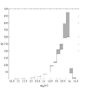
Figure 5: Distribution of the $r$-band Petrosian magnitude of the 1817 galaxies. The shaded region indicates galaxies with small angular sizes ($a_{90}<25$pixels) and unclassified galaxies which were removed from consideration (396 in total).

The $r$-band image is used to compute the concentration index. We use the original image without rescaling, since the seeing effects on the concentration index are small for our bright galaxy sample. The coarseness parameter is computed using the $g$-band image because this filter is generally thought to be more sensitive to texture than $r$-band data (Our experiments have shown, however, that the use of the $r$-band image leads to very little difference in classification). We set the reference size of the semimajor axis to $a_{\rm 90}^{\rm ref}$ = 25 pixels (=$10^{\prime\prime}$; Gunn et al., 1998) and exclude all galaxies with smaller semimajor axes from consideration. This selection for the reference size of the semimajor axis was found to be appropriate for the computation of the coarseness parameter, as galaxies of larger sizes rescaled to 25 pixels retain enough detail for effective classification. In addition, we exclude 23 morphologically disturbed galaxies of class $T$=$-1$ (unclassified by Fukugita et al.) from further analysis. Figure 4 shows the galaxy size distribution measured in the $g$-band, and the shaded areas represent the objects eliminated by the size cutoff and $T$=$-1$ class. This selection leaves the 1421 galaxies in our sample, primarily removing galaxies of earlier types. Galaxies of later types (including irregular galaxies) generally have larger size in a magnitude-limited sample, and are little affected by the size cutoff (see Table 1). The effect of this size cutoff on the $r$-band limited sample is displayed in Figure 5. This selection certainly causes a bias in the ratio among the number of morphological types, but we are not concerned in this paper with issues of completeness and statistics of the number distribution of morphology.

We fix FWHM of the seeing at 3.53 pixels ($1.40^{\prime\prime}$; the median of our sample) and the observed sky noise $\varsigma$ at 4.0 counts for rescaling to simplify our analysis. Since our sample contains bright galaxies whose $a_{\rm 90}$ is near $a_{\rm 90}^{\rm ref}$ and variations of the seeing and $\varsigma$ are sufficiently small, this simplification does not seriously affect the results. In order to assure the independence of the coarseness parameter on galaxy size, we rescale all images to $a_{\rm 90}^{\rm ref}$=25. Extending the analysis to smaller and fainter galaxies will require proper account of the image-to-image variations in seeing and sky noise.

5 PHOTOMETRIC PARAMETERS AND THE MORPHOLOGICAL TYPE

Here we investigate the behavior of the three photometric parameters (circular and elliptical concentration index and coarseness) as a function of the visual morphological type, as quantified by the morphological index $T$. We also show the effect of the axis ratio on these parameters.

5.1 Concentration parameters

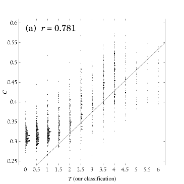
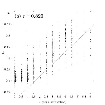
Figure 6: The concentration indices of the 1421 galaxies in our sample versus the visual morphology index $T$. In panel (a) we use the standard circular aperture definitions from the SDSS DR1 catalog for computing the concentration index; in panel (b) we use elliptical apertures. Some points were shifted to larger $T$ values to avoid overlaps. The linear correlation coefficient is given in the top left corner of each panel. The dotted line is an arbitrary line placed in the same position in both panels to facilitate comparison.

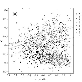
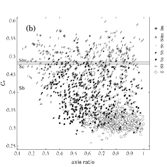
Figure 7: Concentration index versus axis ratio using circular (a) and elliptical (b) aperture definitions. Each symbol indicates visual classification $T$ as specified in the legend, and the straight lines are the linear regression lines for types Sb, Sc and Sdm.

We show that smaller axis ratio affects the standard concentration index $C=r_{50}/r_{90}$ defined with the Petrosian flux in the circular apertures, and using the elliptical ones can remove the effect significantly.

In Figure 6 we plot the two concentration indices against visual morphological type index $T$, calculated by (a) conventional circular apertures ($C$), and (b) elliptical apertures ($C_{e}$). Galaxies that follow de Vaucouleurs’ law give $C$=$C_{e}$=$0.29$ and those with the exponential profile give 0.44.

The Spearman correlation coefficient with the use of $C$, $r$=$0.781$ increases to $r$=$0.820$ with $C_{e}$. Several significant improvements are obtained by the use of an elliptical aperture ($C_{e}$) compared with the original circular aperture ($C$). From Figure 6, the number of spiral galaxies visually classified as $T$=$3$ and $T$=$3.5$ under the dotted line is smaller elliptical than circular concentration index estimates. This is expected for inclined later galaxy types since according to our definition less concentrated galaxies have larger concentration indices. The sample which exhibits larger difference between panel (a) and (b) in Figure 6 contains a significant number of edge-on spirals, which are misclassified using the circular aperture, but correctly identified as less concentrated using the elliptical aperture estimates. A similar improvement is also seen for Sa galaxies ($T$=2).

Thus, using elliptical aperture concentration indices for morphological classification increases the classification accuracy by making it independent of galaxy inclination. In Figure 7 we present the concentration index versus the axis ratio (smaller axis ratios are indicative of larger inclinations) for both the circular (panel (a)) and elliptical aperture (panel (b)) concentration indices. The regression lines are drawn for morphological classes of galaxies Sb, Sc and Sdm. The lines obtained by regression on samples of different galaxy types in panel (a), which are based on $C$, are significantly tilted with respect to the axis ratio. The concentration indices of highly-inclined late-type galaxies estimated using circular apertures are artificially reduced to values characteristic of elliptical morphologies. That is, edge-on spirals give an anomalously high concentration of light if defined with circular apertures; the morphological classifications that use only $C$ have significant contaminants. Figure 7(b), using $C_{e}$, shows that elliptical apertures remedy this problem. We observe little tilt of the regression lines, suggesting that $C_{e}$ works better to classify morphologies than $C$; the effect of inclination is removed with the use of elliptical apertures.

5.2 Coarseness parameter

$Y$=0.00600	$Y$=0.00626	$Y$=0.00667	$Y$=0.00695
(S0;$T$=1)	(E;$T$=0)	(S0;$T$=0.5)	(S0;$T$=0.5)
$Y$=0.00737	$Y$=0.00740	$Y$=0.00743	$Y$=0.00749
(S0;$T$=0.5)	(E;$T$=0)	(E;$T$=0)	(S0;$T$=0.5)
$Y$=0.00750	$Y$=0.00753	$Y$=0.00760	$Y$=0.00788
(S0;$T$=0.5)	(S0;$T$=0.5)	(S0;$T$=0.5)	(E;$T$=0)
$Y$=0.00795	$Y$=0.00798	$Y$=0.00799	$Y$=0.00805
(E;$T$=0)	(S0;$T$=0.5)	(E;$T$=0)	(S0;$T$=0.5)

Figure 8: Rescaled $g$-band images of the 16 galaxies with the lowest coarseness parameters in our sample ($Y\leq 0.00805$). The visually classified morphological types are shown in brackets together with the quantitative morphological index $T$.

$Y$=0.378	$Y$=0.336	$Y$=0.330	$Y$=0.321
(Sc;$T$=4)	(Sc;$T$=4)	(Im;$T$=6)	(Sdm;$T$=5)
$Y$=0.321	$Y$=0.304	$Y$=0.303	$Y$=0.293
(Sc;$T$=3.5)	(Sc;$T$=3.5)	(Sc;$T$=4)	(Sc;$T$=4)
$Y$=0.290	$Y$=0.275	$Y$=0.273	$Y$=0.269
(Sdm;$T$=4.5)	(Sc;$T$=4)	(Sc;$T$=4)	(Sc;$T$=4)
$Y$=0.268	$Y$=0.266	$Y$=0.264	$Y$=0.260
(Sc;$T$=3.5)	(Sc;$T$=3.5)	(Sc;$T$=3.5)	(Im;$T$=6)

Figure 9: Rescaled $g$-band images of the 16 galaxies with the largest coarseness parameters in our sample ($0.260\leq Y$). The visually classified morphological types are shown in brackets together with the quantitative morphological index $T$.

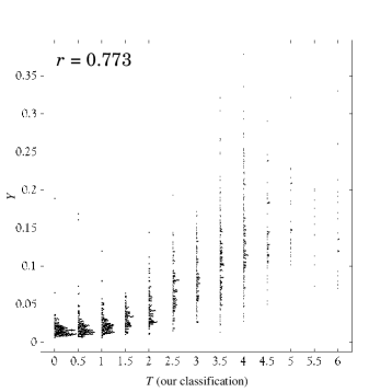
Figure 10: The coarseness parameter $Y$ of the 1421 galaxies in our sample versus the visual morphology index $T$. Some points were shifted to larger $T$ values to avoid overlaps. The linear correlation coefficient is given in the top left corner of the panel.

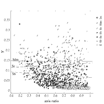
Figure 11: The coarseness parameter $Y$ plotted against the axis ratio. Each symbol indicates visual morphological type, and straight lines are the linear regression for Sb, Sc and Sdm galaxies.

The coarseness parameter $Y$, as defined in equation (17), is equal to the ratio of the range of fluctuations in surface brightness (along an elliptical circumference) to the full dynamic range of surface brightness. Larger values of $Y$ are indicative of the presence of structure in the galaxy disks (e.g., spiral arms) and are associated with galaxies visually classified as late types. Figures 8 and 9 each display 16 galaxies with the smallest ($Y$$<$$0.00805$) and the largest ($Y$$>$$0.260$) $Y$ parameters present in our sample. It is apparent that the galaxies shown in Figure 8 possess very weak texture and are classified as early types. All galaxies shown in Figure 9 have conspicuous texture and are indeed classified as late (Sbc or later)-type spirals.

It is obvious that texture of galaxies contributes to the numerator of equation (17). We should, however, emphasize the role of the denominator. When galaxies have conspicuous bulges, their $\Delta I$ values suppress the $Y$ parameter. On the other hand, the faint bulge leads to a small $\Delta I$ value that enhances $Y$. A typical example of the importance of the denominator of equation (17) is a type of galaxy known as a Magellanic irregular. The texture of Magellanic irregulars is not conspicuous, but the overall intensity contrast is also small, resulting in a small denominator in equation (17) and large $Y$ parameter indicative of a very late type.

Figure 10 displays the coarseness parameter $Y$ plotted against $T$. The correlation ($r$=$0.773$) is not very impressive compared to that for $C_{e}$-$T$, since the $Y$-$T$ correlation is curved away from the linear relation. The important feature in this figure is a very narrow distribution of the $Y$ parameter for 0$\leq$$T$$\leq$1 galaxies. The distribution is confined to the range 0$\leq$$Y$$\lesssim$0.03, which is but 10% of the full variation of $Y$.

The relation between the $Y$ and axis ratio is shown in Figure 11. The linear regression lines for different $T$ are almost flat. They do not appear as flat as those for $C_{e}$, but the slopes of the lines are not caused by any systematic effects, i.e., Sdm is almost flat and Sc/Sb have opposite slopes. We conclude that $Y$ is not affected severely by the inclination of galaxies.

6 MORPHOLOGICAL CLASSIFICATIONS USING $C_{(e)}$ and $Y$ INDICES

6.1 Early versus late types

Figure 12: Completeness $P$ and contamination $Q$ for the early- and late-type galaxy samples as a function of the division parameter $C_{1}$ with the standard circular aperture definition. The thick solid and dotted lines show completeness for early- and late-types. The thin solid and dotted lines show contamination for early- and late-types.

We first attempt to classify galaxies into two types, early (E-S0/a) and late (Sa-Im), by setting a dividing value for each of three parameters displayed in Figure 6(a,b) and Figure 10. We call the two classes of the sample ‘$e$’ and ‘$\ell$’. We evaluate the completeness $P$ and the contamination $Q$ of the ‘$e$’ and ‘$\ell$’, as defined by

$$P_{e}=\frac{N_{e\{{\rm E+S0\}}}}{N_{\rm\{E+S0\}}}~{},~{}~{}~{}Q_{e}=\frac{N_{e{\rm\{Sa+Sb+Sc+Sdm+Im\}}}}{N_{e}}~{},$$ (23)

$$P_{\ell}=\frac{N_{\ell{\rm\{Sa+Sb+Sc+Sdm+Im\}}}}{N_{\rm\{Sa+Sb+Sc+Sdm+Im\}}}~{},~{}~{}~{}Q_{\ell}=\frac{N_{\ell{\rm\{E+S0\}}}}{N_{\ell}}~{},$$ (24)

where $N_{e}$ is the number of all galaxies chosen by the separator line, $N_{e{\{{\rm E+S0}\}}}$ is the number of E+S0 galaxies chosen by the separator line, and $N_{\{{\rm E+S0}\}}$ is the total number of E+S0 galaxies. Other notations are defined similarly.

Figure 13: Completeness $P$ and contamination $Q$ of the early- and late-type galaxy samples as a function of the division parameter $C_{e1}$, defined using elliptical apertures. See Figure 12 for the line definitions.

Figure 14: Completeness $P$ and contamination $Q$ of the early- and late-type galaxy samples as a function of the division parameter $Y_{1}$. See Figure 12 for the line definitions.

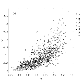
Figure 15: (a) 1421 Galaxies plotted on the ($C_{e}$,$Y$) plane and (b) the average 2-vector and standard deviation for each morphological class. The solid line in panel (b) is the quadratic function least-squares fit to the points representing the average values for each morphological class. The two dot-dashed lines are the best classifiers into three types, E+S0, Sa+Sb and Sc+Sdm+Im using the 2-dimensional classification. The dotted and dashed lines show the best one dimensional separators using $C_{e}$ and $Y$, respectively.

Figure 12 shows completeness and contamination for the classification using the $C$ parameter. The same analysis is performed in Shimasaku et al. (2001) which attains 80% completeness at $C_{1}$=$0.35$. Strateva et al. (2001) also reports 83% completeness at $C_{1}$=$0.38$ using a concentration index with circular apertures. We find that $P_{e}$=$P_{\ell}$=$85.0$%, $Q_{e}$=$22.5$% and $Q_{\ell}$=$9.5$% with the use of the division constant $C_{1}$=$0.339$. The success rate is somewhat higher in our case, however, with essentially the same division parameter. Improved performance is seen in Figure 13 where the $C$ parameter is replaced with $C_{e}$: we obtain $P_{e}$=$P_{\ell}$=$86.7$%, $Q_{e}$=$20.0$% and $Q_{\ell}$=$8.2$% for $C_{e1}$=$0.349$. One may attain $Q_{e}$=$Q_{\ell}$=$15.0\%$ with the choice of $C_{e1}$=$0.332$ if the completeness of E+S0 galaxies is sacrificed.

Figure 16: Completeness and contamination of the early and late-type galaxy samples as a function of $C_{e1}$ specified at the crossing point with the quadratic function, using the $C_{e}$-$Y$ diagram (Figure 15). See Figure 12 for the line definitions.

The result of classification using the $Y$ parameter is presented in Figure 14. This result shows a higher success rate than the $C_{e}$ classification, $P_{e}$=$P_{\ell}$=$88.1\%$, $Q_{e}$=$18.1$% and $Q_{\ell}$=$7.5\%$ for $Y_{1}$=$0.030$. We can attain minimum contamination of $Q_{e}$=$Q_{\ell}$=$12.1\%$ for $Y_{1}$=$0.024$ with a modest cost of $P_{e}$. We conclude that the $Y$ parameter is superior to the concentration indices as the morphology classifier.

We now try to obtain the maximum performance using two parameters, $C_{e}$ and $Y$, by optimising the choice of the dividing parameters (see Figure 15). We consider the position of the center of the average 2-vector for each morphological class,

$${G}_{\rm E}=\left(\matrix{\langle{{C_{e}}_{\rm E}}\rangle\cr\langle{Y_{\rm E}\rangle}}\right),~{}{G}_{\rm S0}=\left(\matrix{\langle{{C_{e}}_{\rm S0}}\rangle\cr\langle{Y_{\rm S0}\rangle}}\right),$$

$$...,~{}{G}_{\rm Im}=\left(\matrix{\langle{{C_{e}}_{\rm Im}}\rangle\cr\langle{Y_{\rm Im}\rangle}}\right).$$ (25)

where $\langle{{C_{e}}_{\rm E}}\rangle=(1/N_{\rm E})\sum_{i\in{\rm E}}{{C_{e}}_{\rm E}^{i}}$ etc. With the weight of the number of the galaxies having the relevant morphological class given to these points, we fit 7 points by a quadratic function. For our 1421 galaxies, we obtain

$$f_{q}(C_{e})=2.702C_{e}^{2}-1.419C_{e}+0.1967.$$ (26)

In general, for 2-D distributions that show separate linear correlations for each type, the separator lines are parallel to the individual correlations (see Doi et al. 1993). We apply this method to the quadratic regression line. We then consider a set of lines crossing this quadratic curve at $(C_{e1},f_{q}(C_{e1}))$,

$$f_{l}(C_{e})=-\frac{K}{f_{q}^{\prime}(C_{e1})}(C_{e}-C_{e1})+f_{q}(C_{e1})$$ (27)

where $K$ is a constant, and $f_{q}^{\prime}$ is the first derivative of $f_{q}$. We take $f_{l}(C_{e})$ as the dividing line for classification. We adopt $K$=$0.1$, which turns out to give the best performance. Figure 15 shows the average 2-vector and standard deviation for each morphological class, the quadratic regression $f_{q}(C_{e})$ and the best separator line between the early and late type galaxies (lower dot-dashed line).

The completeness and contamination curves for classification using the $C_{e}$-$Y$ diagram are presented in Figure 16. The maximum success rate we achieved is (assuming equal completeness for both early and late types) $P_{e}$=$P_{\ell}$=$89.4\%$, with $Q_{e}$=$16.4\%$ and $Q_{\ell}$=$6.7\%$ for $C_{e1}$=$0.348$, or (assuming equal contamination) $P_{e}$=$79.3$% and $P_{\ell}$=$93.6$% with $Q_{e}$=$Q_{\ell}$=$11.8\%$ for $C_{e1}$=$0.337$. These are remarkably high success rates given the fact that visual classification suffers from uncertainties, perhaps of the order $\Delta T\sim 1$.

6.2 Classification into three types

$C$ Parameter
	E+S0	Sa+Sb	Sc+Sdm+Im	Total
$e$	458	124	9	591
$\ell_{\rm I}$	76	278	161	515
$\ell_{\rm II}$	3	59	253	315
Total	537	461	423	1421
$C_{e}$ Parameter
	E+S0	Sa+Sb	Sc+Sdm+Im	Total
$e$	468	111	6	585
$\ell_{\rm I}$	68	285	156	509
$\ell_{\rm II}$	1	65	261	327
Total	537	461	423	1421
$Y$ Parameter
	E+S0	Sa+Sb	Sc+Sdm+Im	Total
$e$	474	99	6	579
$\ell_{\rm I}$	59	305	138	502
$\ell_{\rm II}$	4	57	279	340
Total	537	461	423	1421

Table 2: Classification of 1421 galaxies into three types (E+S0 : Sa+Sb : Sc+Sdm+Im) using parameter $C$,$C_{e}$, or $Y$. The completeness of a selection method can be calculated using the numbers from each column as follows. For the selection method using $C$, the completeness of the E+S0 sample is 458/537$\simeq$0.85 (from column 1 of the $C$ table), and the contamination is (124+9)/591$\simeq$0.23 (from row 1 of the $C$ table).

$C_{e}$-$Y$ Diagram
	E+S0	Sa+Sb	Sc+Sdm+Im	Total
$e$	480	92	2	574
$\ell_{\rm I}$	53	314	137	504
$\ell_{\rm II}$	4	55	284	343
Total	537	461	423	1421

Table 3: Classification of 1421 galaxies into three types (E+S0/Sa+Sb/Sc+Sdm+Im) using the $C_{e}$-$Y$ diagram. The completeness of a selection method can be calculated using the numbers from each column as follows. The completeness of E+S0 sample in the $e$ is 480/537$\simeq$0.89 (from column 1), and the contamination of the $e$ is (92+2)/574$\simeq$0.16 (from row 1).

We consider separation into three types, dividing late (‘$\ell$’)- type galaxies into early ($\sim$ Sa+Sb) and late spirals ($\sim$ Sc+Sdm+Im). We call the two classes of the sample $\ell_{\rm I}$ and $\ell_{\rm II}$. We fix the first division for the early/late classification as determined in the previous subsection. We set the second division which separates $\ell_{\rm I}$ and $\ell_{\rm II}$ so that the completeness of Sa+Sb in $\ell_{\rm I}$ and that of Sc+Sdm+Im in $\ell_{\rm II}$ are nearly equal.

We show the results in matrices of $3\times 3$ (and an additional row and column to show the subtotals) in Table 2 for the three indicators using $C$, $C_{e}$ and $Y$. We take the second division separators which divide late-type galaxies into early- and late-spirals to be $C_{2}$=$0.436$, $C_{e2}$=$0.463$, and $Y_{2}$=$0.106$, respectively, while the separators between early- and late-type galaxies are the same as those quoted in the beginning of Section 6.1. The completeness can be read from the column by dividing the number in the diagonal entry by the total number of listed in the bottom of the corresponding column. For example, the completeness of Sa+Sb galaxies separated by $C_{1,2}$ is $278/461=60.3$%. This compares to $285/461=61.8$% with the use of $C_{e}$, and $305/461=66.2$% with $Y$. The contamination is read from the row. The contamination in the early spiral galaxy sample, $\ell_{\rm I}$, from E+S0 galaxies and late-type spiral galaxies, for instance, is $(76+161)/515=46.0$% with the use of $C$, $(68+156)/509=44.0$% with $C_{e}$, and $(59+138)/502=39.2$% with $Y$. Similarly the $\ell_{\rm II}$ contamination is $20.0$%, $20.2$%, and $17.9$%, for the $C$, $C_{e}$, and $Y$ parameter classification, respectively.

The classification with $Y$ again produces the best result. We also note that the gain attained with the use of elliptical apertures over circular apertures is small for $\ell_{\rm I}$ and $\ell_{\rm II}$, although the $C_{e}$ parameter gives generally better performance, if slight. One might question why the gain with $C_{e}$ over $C$ is rather small in contrast to the emphasis given in the previous section that using $C_{e}$ parameter removed the effect of inclination. The reason is that early and late spiral galaxies are not well separated in the concentration parameter space, and show large dispersion with heavy overlaps. So the effect of inclination does not play a crucial role. In fact, visual separation into early and late spirals relies more on the opening of spiral arms and texture.

It is important to note that contaminants from late spirals to the early-type sample, or vice versa, are very small, less than $\lesssim 1$%, at least with the $C_{e}$ and $Y$ indices. Most of the contaminants in the E+S0 sample are from S0a and Sa galaxies.

Finally, we examine how the performance of our morphology classifier improves by considering 2-dimensional classification in the $C_{e}$-$Y$ space. The result is shown in Table 3. The completeness of the Sa+Sb galaxy sample is $314/461=68.1$%, a 2% increase, compared with the value found employing $Y$ alone. The contamination in the $\ell_{\rm I}$ sample from E+S0 galaxies and late-type spiral galaxies decreases to $(53+137)/504=34.1$%, which is 5% smaller than the value obtained by using $Y$ alone. The contamination in the early-type spiral sample still primarily arises from late-type spiral galaxies, rather than E+S0 galaxies. The contamination in the $\ell_{\rm II}$ sample decreases from 17.9% to 17.2%.

7 CONCLUSIONS

We started by examining the standard concentration index $C=r_{50}/r_{90}$, defined using the Petrosian flux in circular apertures, and found that the correlation is significantly affected by galaxy inclination. The value of the standard concentration index $C$ of a highly inclined spiral is artificially reduced (i.e. the galaxy appears to have more centrally concentrated light) and the galaxy is misclassified as an early type. We found that this inclination dependence vanishes if we define the concentration index using elliptical apertures. The ellipse-based concentration index $C_{e}$ calculated from the Petrosian flux gives an inclination-independent indicator.

In addition, we devised a new texture parameter, $Y$, that represents the coarseness of surface brightness. The $Y$ parameter measures the texture of a galaxy disk in relation to the galaxy’s overall surface brightness contrast (including the galaxy bulge). It is defined in a manner that closely mimics visual classification. Late type spiral galaxies (which often show distinct spiral arms) or Magellanic type irregulars (whose disks are less pronounced but so are their bulges) both have large $Y$ values, in contrast to early type galaxies. We found that the $Y$ parameter of a galaxy is strongly correlated with its visual morphology.

We investigated the performance of the three different photometric parameters ($C$, $C_{e}$, and $Y$) for morphological classification into two (E+S0 and Sa+Sb+Sc+Sdm+Im) or three (E+S0, Sa+Sb, and Sc+Sdm+Im) galaxy types. In both cases we found that the elliptical aperture classifier, $C_{e}$, is better than the standard circular aperture classifier, $C$. The coarseness parameter, $Y$, produces results superior to those obtained with either of the concentration index parameters. Depending on the desired balance between completeness and contamination, sample completeness as high as 88% or contamination as low as 12% is achievable.

We can further improve the classification by considering 2-dimensional (using the $C_{e}$-$Y$ plane) classification. In the case of classification into two morphological types, this allows us to attain a 89% completeness and contamination as low as 12%. For classification into three morphological types, the completeness is 68%.

Our newly devised photometric parameter, coarseness, provides a mode of morphological classification as good as the traditionally used human-eye classification. At the same time, it is fully automated, and thus, can be used quite easily for millions of galaxies. Therefore, the coarseness parameter presented in this paper has a potential to open new doors to detailed studies of galaxy morphology in current and future large CCD surveys.

References

- Abazajian et al. (2003) Abazajian, K., et al. 2003, AJ, 126, 2081
- Abazajian et al. (2004) Abazajian, K., et al. 2004, AJ, 128, 502
- Abraham et al. (1996) Abraham, R. G., van den Bergh, S., Glazebrook, K., Ellis, R. S., Santiago, B. X., Surma, P., & Griffiths, R. E. 1996, ApJS, 107, 1
- Abraham et al. (1994) Abraham, R. G., Valdes, F., Yee, H. K. C., & van den Bergh, S. 1994, ApJ, 432, 75
- Ball et al. (2004) Ball, N. M., Loveday, J., Fukugita, M., Nakamura, O., Okamura, S., Brinkmann, J., & Brunner, R. J. 2004, MNRAS, 348, 1038
- Binggeli, Sandage & Tammann (1988) Binggeli, B., Sandage, A., & Tammann, G. A. 1988, ARA&A, 26, 509
- Brinchmann et al. (1998) Brinchmann, J., et al. 1998, ApJ, 499, 112
- Burda & Feitzinger (1992) Burda, P. & Feitzinger, J. V. 1992, A&A, 261, No.2, 697
- Dressler (1980) Dressler, A. 1980, ApJ, 236, 351
- Dressler (1994) Dressler, A., Oemler, A. J., Sparks W. B., Lucas, R. A. 1994, ApJ, 435, L23
- Doi, Fukugita & Okamura (1993) Doi, M., Fukugita, M., & Okamura, S. 1993, MNRAS, 264, 832
- Fukugita et al. (1996) Fukugita, M., Ichikawa, T., Gunn, J. E., Doi, M., Shimasaku, K., & Schneider, D. P. 1996, AJ, 111, 1748
- Gunn et al. (1998) Gunn, J. E., et al. 1998, AJ, 116, 3040
- Hogg et al. (2001) Hogg, D. W., Schlegel, D. J., Finkbeiner, D. P., & Gunn, J. E. 2001, AJ, 122, 2129
- Lupton et al. (2001) Lupton, R. H., Gunn, J. E., Ivezic, Z., Knapp, G. R., Kent, S., & Yasuda, N. 2001, Astronomical Data Analysis Software and Systems X, ASP Conference Proceedings, 238, 269
- Lupton (1996) Lupton, R. H., 1996, SDSS Web Site 444) http://www.astro.princeton.edu/∼rhl/photomisc/ellipticity.ps), The Estimation of Object’s Ellipticities.
- Naim, Ratnatunga & Griffiths (1997) Naim, A., Ratnatunga, K. U., & Griffiths, R.E. 1997, ApJ, 476, 510
- Naim et al. (1995) Naim, A., Lahav, O., Sodre, L., & Storrie-Lombardi, M. C. 1995, MNRAS, 275, 567
- Nakamura et al. (2003) Nakamura, O., Fukugita, M., Yasuda, N, Loveday, J., Brinkmann, J., Schneider, D. P., Shimasaku, K., SubbaRao, M. 2003, AJ, 125, 1682
- Morgan (1958) Morgan, W. W. 1958, PASP, 70, 364
- Odewahn et al. (2002) Odewahn, S. C., Cohen, S. H., Windhorst, R. A., & Philip, N. S. 2002, ApJ, 568, 539
- Pier et al. (2003) Pier, J. R., Munn, J. A., Hindsley, R. B., Hennessy, G. S., Kent, S. M., Lupton, R. H., & Ivezic, Z. 2003, AJ, 125, 1559
- Sandage (1961) Sandage, A. 1961, The Hubble Atlas of Galaxies (Washington: Carnegie Inst. Washington)
- Serra-Ricart et al. (1993) Serra-Ricart, M., Calbet, X., Garrido, L., & Gaitan, V. 1993, AJ, 106, 1685
- Shimasaku et al. (2001) Shimasaku, K., et al. 2001, AJ, 122, 1238
- Smith et al. (2002) Smith, J. A., et al. 2002, AJ, 123, 2121
- Storrie-Lombardi et al. (1992) Storrie-Lombardi, M. C., Lahav, O., Sodre, L., & Storrie-Lombardi, L. J. 1992, MNRAS, 259, 8p
- Stoughton et al. (2002) Stoughton, C., et al. 2002, AJ, 123, 485
- Strateva et al. (2001) Strateva, I., et al. 2001, AJ, 122, 1861
- Strauss et al. (2002) Strauss, M. A. et al. 2002, AJ, 124, 1810
- Takamiya (1999) Takamiya, M. 1999, ApJS, 122, 109
- York et al. (2000) York, D. G., et al. 2000, AJ, 120, 1579