Topology Analysis of the Sloan Digital Sky Survey:
I. Scale and Luminosity Dependence

Abstract

We measure the topology of volume-limited galaxy samples selected from a parent sample of 314,050 galaxies in the Sloan Digital Sky Survey (SDSS), which is now complete enough to describe the fully three-dimensional topology and its dependence on galaxy properties. We compare the observed genus statistic $G(\nu_{f})$ to predictions for a Gaussian random field and to the genus measured for mock surveys constructed from new large-volume simulations of the $\Lambda$CDM cosmology. In this analysis we carefully examine the dependence of the observed genus statistic on the Gaussian smoothing scale $R_{G}$ from 3.5 to 11 $\,h^{-1}{\rm Mpc}$ and on the luminosity of galaxies over the range $-22.50<M_{r}<-18.5$. The void multiplicity $A_{V}$ is less than unity at all smoothing scales. Because $A_{V}$ cannot become less than 1 through gravitational evolution, this result provides strong evidence for biased galaxy formation in low density environments. We also find clear evidence of luminosity bias of topology within the volume-limited sub-samples. The shift parameter $\Delta\nu$ indicates that the genus of brighter galaxies shows a negative shift toward a “meatball” (i.e. cluster-dominated) topology, while faint galaxies show a positive shift toward a “bubble” (i.e. void-dominated) topology. The transition from negative to positive shift occurs approximately at the characteristic absolute magnitude $M_{r*}=-20.4$. Even in this analysis of the largest galaxy sample to date, we detect the influence of individual large-scale structures, as the shift parameter $\Delta\nu$ and cluster multiplicity $A_{C}$ reflect (at $\sim 3\sigma$) the presence of the Sloan Great Wall and a $x$-shaped structure which runs for several hundred Mpc across the survey volume.

1. Introduction

Topology analysis was introduced in cosmology as a method to test Gaussianity of the primordial density field as predicted by many inflationary scenarios (Gott, Melott, & Dickinson 1986). The statistics of the initial density field are thought to be well preserved at large scales where structures are still in the linear regime. Therefore, to achieve the original purpose of topology analysis one needs to use large observational samples and explore the galaxy density field at large smoothing scales. This requires an accurate map of the large-scale distribution of galaxies over scales of several hundred megaparsecs, as is now available from the Sloan Digital Sky Survey (SDSS).

On smaller scales in the non-linear regime, the topology of the galaxy distribution yields strong constraints on the galaxy formation mechanisms and the background cosmogony. Galaxies of various species are distributed in different ways in space, and the differences can be quantitatively measured by topology analysis. By studying galaxy biasing as revealed in statistics beyond the two-point correlation function and power spectrum, the complex nature of galaxy formation can be better understood. The topology statistics can be precision measures of the galaxy formation process (Park, Kim, & Gott 2005). To examine topology at small scales it is necessary to use dense galaxy redshift samples which are also large enough in volume to not to be significantly affected by sample variance. Using the SDSS, it is now possible to study the topology of the galaxy distribution down to a Gaussian smoothing scale of $3\,h^{-1}{\rm Mpc}$ scale in volume-limited samples that include galaxies as faint as absolute magnitude $M_{r}=-18$, while still maintaining reasonably large sample volumes.

Previous topological analysis of SDSS galaxy distribution include the 2D genus (Hoyle et al. 2002), 3D genus with Early Data Release (Hikage et al. 2002), and Minkowski Functionals with Sample 12 (Hikage et al. 2003). The present paper updates the previous results with the latest SDSS sample, describe below as Sample 14. For the first time, we are able to detect the quantitative signature of luminosity-dependent biasing by characterizing the genus curves in terms of the statistical quantities, $\Delta\nu$, $A_{V}$, and $A_{C}$. $\Delta\nu$ is shift parameter and $A_{V}$ and $A_{C}$ are cluster and void abundance parameters, respectively.

In this paper we adopt the genus statistic as a measure of the topology of the smoothed galaxy number density field. To study the impact of galaxy biasing, we limit our attention to small-scale topology, over a range of Gaussian smoothing scales of from 3.5 to 11 $\,h^{-1}{\rm Mpc}$. We examine the scale-dependence of topology to see if there are differences with respect to the $\Lambda{\rm CDM}$ model. We also detect the luminosity bias in the topology of large scale structure. In section 2 we briefly describe the SDSS and define our volume-limited SDSS samples. In section 3 we define the topology statistics and describe our genus analysis procedure. Section 4 describes our new N-body simulation, which we use for constructing mock surveys and testing for systematic effects. In section 5 we present results of tests for scale and luminosity dependences of the observed genus curves. We discuss our findings in section 6.

2. Observational Data Set

2.1. Sloan Digital Sky Survey

The SDSS (York et al. 2000; Stoughton et al. 2002; Abazajian et al. 2003; Abazajian et al. 2004) is a survey to explore the large scale distribution of galaxies and quasars, and their physical properties by using a dedicated $2.5{\rm m}$ telescope at Apache Point Observatory. The photometric survey, which is expected to be completed in June 2005, will image roughly $\pi$ steradians of the Northern Galactic Cap in five photometric bandpasses denoted by $u$, $g$, $r$, $i$, and $z$ centered at $3551,4686,6165,7481,$ and $8931\AA$, respectively by an imaging camera with 54-CCDs (Fukugita et al. 1996; Gunn et al. 1998). The limiting magnitudes of photometry at a signal-to-noise ratio of $5:1$ are $22.0,22.2,22.2,21.3$, and $20.5$ in the five bandpasses, respectively. The width of the PSF is $1.4\arcsec$, and the photometric uncertainties are $2\%$ rms (Abazajian et al. 2004). Roughly $5\times 10^{7}$ galaxies will be cataloged.

After image processing (Lupton et al. 2001; Stoughton et al. 2002; Pier et al. 2003) and calibration (Hogg et al. 2001; Smith et al. 2002), targets are selected for spectroscopic follow-up observation. The spectroscopic survey is planned to continue through 2008 as the Legacy survey, and produce about $10^{6}$ galaxy spectra. The spectra are obtained by two dual fiber-fed CCD spectrographs. The spectral resolution is $\lambda/\Delta\lambda\sim 1800$, and the r.m.s. uncertainty in redshift is $\sim 30$ km/s. Mainly due to the minimum distance of $55\arcsec$ between fibers, incompleteness of spectroscopic survey reaches about 6% (Blanton et al. 2003a) in such a way that regions with high surface densities of galaxies become less prominent. This angular variation of sampling density is accounted for in our analysis.

The SDSS spectroscopy yields three major samples: the main galaxy sample (Strauss et al. 2002), the luminous red galaxy sample (Eisenstein et al. 2001), and the quasar sample (Richards et al. 2002). The main galaxy sample is a magnitude-limited sample with apparent Petrosian $r$-magnitude cut of $m_{r,\mathrm{lim}}\approx 17.77$ which is the limiting magnitude for spectroscopy (Strauss et al. 2002). It has a further cut in Petrosian half-light surface brightness $\mu_{\rm{R50},\mathrm{limit}}=24.5$ mag/arcsec². More details about the survey can be found at http://www.sdss.org/dr3/.

In our topology analysis, we use a large-scale structure sample of the SDSS from the NYU Value-Added Catalog (VAGC, Blanton et al. 2004). As of the writing of this paper, the most up-to-date large-scale structure sample is Sample 14, which covers 3,836 square degrees of the sky, and contains 314,050 galaxies between redshift of $0.001$ and $0.5$, surveyed as of November 2003. The large-scale structure sample also comes with an angular selection function of the survey defined in terms of spherical polygons (Hamilton & Tegmark 2004), which takes into account the incompleteness due to mechanical spectrograph constraints, bad spectra, or bright foreground stars.

2.2. Sample Definitions for Genus Analysis

To study the three-dimensional topology of the smoothed galaxy number density distribution, it is advantageous for the observational sample to have the lowest possible surface-to-volume ratio. For this reason we trim Sample 14 as shown in Figure 1, where the solid lines delineate our sample boundaries in the survey coordinate plane ($\lambda,\eta$). We discard the three southern stripes and the small areas protruding or isolated from the main surveyed regions. These cuts decrease the number of galaxies from 314,050 to 239,216 in two analysis regions. Within our sample boundaries, we account for angular variation of the survey completeness by using the angular selection function provided with the large scale structure sample data set. To facilitate our analysis, we make two arrays of square pixels of size $0.025\arcdeg\times 0.025\arcdeg$ in the ($\lambda,\eta$) sky coordinates which cover the two analysis regions, and store the angular selection function calculated by using the mangle routine (Hamilton & Tegmark 2004). At the location of each pixel, the routine calculates the survey completeness in a spherical polygon formed by the adaptive tiling algorithm (Blanton et al. 2003a) used for the SDSS spectroscopy. The resulting useful area within the analysis regions with non-zero selection function is 0.89 steradians.

Analysis region 1 contains the famous “Sloan Great Wall” for which redshift slices are shown by Gott et al. 2003. Figure 2 shows galaxies with $14.5\leq m_{r}\leq 17.5$ in two $7.5\arcdeg$-thick slices in the analysis region 2. We assume a flat $\Lambda{\rm CDM}$ cosmology with $\Omega_{\rm m}=0.3$ to convert redshifts to comoving coordinates. In the upper slice of Figure 2 there is a weak wall of galaxies that extends over $\sim 700\,h^{-1}{\rm Mpc}$ at comoving distance of roughly $r=400\,h^{-1}{\rm Mpc}$. Void, wall, and filamentary structures of galaxies are seen through these slices. A roughly spherical void of size $\sim 100\,h^{-1}{\rm Mpc}$ in diameter is seen in the slices at distance of about $200\,h^{-1}{\rm Mpc}$. In the lower slice there is a $\sim 300\,h^{-1}{\rm Mpc}$ size structure which looks like a runner or a $x$ mark, formed by several neighboring voids of various sizes as was the structure in the CfA slice (Geller & Huchra 1989). We note several small voids nested within larger ones.

In our topology analysis we use only volume-limited samples of galaxies defined by absolute magnitude limits. Figure 3 shows galaxies in Sample 14 in redshift-absolute magnitude space. The smooth curves delineate the sample boundaries corresponding to our choice of apparent magnitude limits of $14.5\leq m_{r}\leq 17.5$, after correction for Galactic reddening (Schlegel, Finkbeiner, & Davis et al. 1998). The faint limit of $m_{r}=17.5$ is slightly brighter than the spectroscopic selection criterion of $m_{r}<17.77$, to allow use of some early data that used a brighter limit. The bright-end apparent magnitude limit of $m_{r}=14.5$ is imposed to avoid small incompleteness that is caused by the exclusion of galaxies with large central surface brightness (to avoid spillover in the spectrograph CCDs) and associated with the quality of deblending of large galaxies. The most natural volume-limited sample is the one containing the maximum number of galaxies. We vary the faint and bright absolute magnitude limits to find such a sample and label this our “Best” sample. It is defined by a absolute-magnitude limits $-21.53\leq M_{r}<-20.15$, which correspond to a comoving distance range of $162.9<r<319.0\,h^{-1}{\rm Mpc}$ or redshift range $0.055<z<0.109$ when the apparent magnitude cut is applied. The comoving distance and redshift limits are obtained by using the formula

$$m_{r}-M_{r}=5{\rm log}(r(1+z))+25+K(z),$$ (1)

where $K(z)$ is the K-correction and $r(1+z)$ is the luminosity distance. We use a polynomial fit to the mean K-correction within $0<z<0.3$,

$$K(z)=2.3537(z-0.1){{}^{2}}+1.04423(z-0.1)-2.5{\rm log}(1+0.1).$$ (2)

The rest-frame absolute magnitudes of galaxies in Sample 14 are computed in fixed bandpasses, shifted to $z=0.1$, using Galactic reddening corrections and K-corrections (for a full description, see Hogg et al. 2002 and Blanton et al. 2003b). This means that galaxies at $z=0.1$ have K-correction of $-2.5{\rm log}(1+0.1)$, independent of their SEDs. We do not take into account galaxy evolution effects. The definition of the ‘Best’ sample is shown in Figure 3 and Table 1.

The upper panel of Figure 3 also shows the absolute-magnitude and redshift limits for two additional samples, which we label “Sparse” and “Dense” because of their mean density relative to the “Best” sample. The Dense sample has a bright absolute magnitude limit just below the faint limit of the Best sample. The faint limit of the Dense sample is determined by maximizing the number of galaxies. For the Sparse sample, the bright absolute magnitude limit was chosen to be fainter than $-22.22$, above which galaxies in Sample 14 are missing at far distances. The faint limit of the Sparse is determined by maximizing the number of galaxies contained in the sample. In what follows these samples are used to study dependence of topology on scale.

The lower panel of Figure 3 shows the absolute-magnitude and redshift limits of four samples that we use to study the luminosity dependence of topology. Each sample has an absolute magnitude range of two magnitudes. The brightest sample, L1, has a bright magnitude limit of $M_{r}=-22.5$. Each luminosity sample is further divided into three subsamples defined as in Table 1. Each subsamples has half the number of galaxies contained in its parent sample, and the brightest subsample does not overlap with the faintest one in absolute magnitude. Because the subsamples occupy the same volume of the universe and contain the same number of galaxies, differences among them are free from sample-variance and Poisson fluctuation; any variation in topology is purely due to difference in the absolute magnitude of the galaxies.

3. Theory for Topology Analysis

3.1. Genus and its Related Statistics

The genus is a measure of the topology of isodensity contour surfaces in a smoothed galaxy density field. It is defined as

$$G={\rm Number~{}of~{}holes~{}in~{}contour~{}surfaces-Number~{}of~{}isolated~{}regions}$$ (3)

in the isodensity surfaces at a given threshold level. The Gauss-Bonnet theorem connects the global topology with an integral of local curvature of the surface $S$, i.e.

$$G={1\over{4\pi}}\int_{S}\kappa da,$$ (4)

where $\kappa$ is the local Gaussian curvature. In the case of a Gaussian field the genus per volume as a function of density threshold level is known (Doroshkevich 1970; Adler 1981; Hamilton, Gott, & Weinberg 1986):

$$g(\nu)=g(0)(1-\nu^{2})e^{-\nu^{2}/2},$$ (5)

where $\nu\equiv(\rho-{\bar{\rho}})/\sigma$ is the threshold density in unit of standard deviations $\sigma=\langle(\rho-{\bar{\rho}})^{2}\rangle^{1/2}$ from the mean. The amplitude is

$$g(0)={1\over{(2\pi)^{2}}}({{\langle k^{2}\rangle}\over 3})^{3/2},$$

where

$${\langle k^{2}\rangle}=\int P(k)k^{2}d^{3}k/\int P(k)d^{3}k$$

depends on the power spectrum $P(k)$ of the smoothed density field. To separate variation in topology from change of the the one-point density distribution we measure the genus as a function of the volume-fraction threshold $\nu_{f}$. This parameter defines the density contour surface such that the volume fraction in the high density region is the same as the volume fraction in a Gaussian random field contour surface with a value of $\nu=\nu_{f}$. Any deviation of the observed genus curve from the Gaussian one is evidence for non-Gaussianity of the primordial density field and/or that acquired due to the nonlinear gravitational evolution or galaxy biasing. There have been a number of studies on the effects of non-Gaussianity on the genus curve (Weinberg et al. 1987; Park & Gott 1991; Park, Kim, & Gott 2005).

To measure the deviation of the genus curve from Gaussian, several statistics have been suggested. First is the amplitude drop, $R=G_{\rm obs}/G_{\rm G}$ where $G_{\rm obs}$ is the amplitude of the observed genus curve and $G_{\rm G}$ is that of a Gaussian field which has the observed power spectrum (Vogeley et al. 1994). It is a measure of the phase correlation produced by the initial non-Gaussianity, the gravitational evolution, and the galaxy biasing. We will not calculate $R$ in this paper and defer it to later works in which we will examine the genus over a larger range of smoothing scales that include the linear regime. Here we simply measure the observed genus amplitude $G_{\rm obs}$ to test for scale and luminosity dependence. $G_{\rm obs}$ is measured by finding the best fitting Gaussian genus curve over $-1\leq\nu\leq 1$.

The shift parameter $\Delta\nu$ is defined as

$$\Delta\nu=\int d\nu G_{\rm obs}(\nu)\nu/\int d\nu G_{\rm fit}(\nu),$$ (6)

where the integral is over $-1\leq\nu\leq 1$, and $G_{\rm obs}$ and $G_{\rm fit}$ are the observed and the best-fit Gaussian genus curves (Park et al. 1992). It measures the threshold level where topology is maximally sponge-like. For a density field dominated by voids, $\Delta\nu$ is positive and we say that the density field has a “bubble-like” topology. For a cluster dominated field, $\Delta\nu$ is negative and we say that the field has a “meatball-like” topology.

The abundances of clusters and voids relative to that expected for a Gaussian random field are measured by the parameters $A_{\rm C}$ and $A_{\rm V}$. These parameters are defined by

$$A=\int d\nu G_{\rm obs}(\nu)/\int d\nu G_{\rm fit}(\nu),$$ (7)

where the integration intervals are $+1.2<\nu_{f}<+2.2$ for $A_{\rm C}$ and $-2.2<\nu_{f}<-1.2$ for $A_{\rm V}$ (Park, Gott, & Choi 2001; Park, Kim, & Gott 2005). These intervals are centered near the minima of the Gaussian genus curve ($\nu=\pm\sqrt{3}$) and stay away from the thresholds where the genus curve is often affected by the shift phenomenon. These ranges also exclude extreme thresholds where for low density regions the volume-fraction threshold level $\nu_{f}$ is very sensitive to the density value. These parameters are defined so that $A_{\rm C,V}>1$ means that more independent clusters or voids are observed than predicted by a Gaussian field at fixed volume fraction, whereas $A_{\rm C,V}<1$ means that fewer independent clusters or voids are seen. A detailed study of the effects of the gravitational evolution, the galaxy biasing, and the cosmogony on the $\Delta\nu$, $A_{\rm V}$, and $A_{\rm C}$ statistics is presented by Park, Kim, & Gott (2005).

3.2. Analysis Procedure

To measure the genus using the contour3D algorithm (Weinberg 1988), we prepare an estimate of the smoothed density field on a grid, with pixels that lie outside the survey region flagged. Figure 1 together with the angular selection function table defines our angular mask. Table 1 lists the distance range for each sample. Using the angular mask and distance limits, we make a three-dimensional mask array of size $512^{3}$ for each sample. The pixel size is always restricted to be slightly smaller than $R_{\rm G}/3$ where $R_{\rm G}$ is the Gaussian smoothing length. The Earth is located at the center of one face of the cubic array that forms the $x$-$z$ plane. This mask array contains zeros in pixels that lie outside the boundaries shown in Figure 1. Mask array pixels that lie within the boundaries are assigned a selection function value read off from the angular selection function table. Because that table consists of fine pixels of $1.5\arcmin$ size, the mask array faithfully represents the survey selection effects. We also make a $512^{3}$ galaxy density array into which we bin the SDSS galaxies which fall inside our sample boundaries. After a Gaussian smoothing length $R_{\rm G}$ is chosen, both the mask array and the galaxy density array are smoothed and divided by each other in the sense of $\rho_{\rm g}/\rho_{\rm mask}$. This yields an array of smoothed galaxy density estimates that accounts for both the angular selection function and the effect of the survey boundary. In regions of the ratio array for which the corresponding value in the smoothed mask array value is smaller than $0.69$, we flag the ratio array with negative values to indicate that they are outside the analysis region. This removes not only regions that are formally outside the survey volume, but also regions that are too close to the survey boundary, where the signal-to-noise ratio of the estimated density field is low. We choose a threshold value of $0.69$ as a compromise between homogeneous smoothing and a larger survey volume. This value corresponds to the value of a smoothed mask at a distance of $0.5R_{\rm G}$ inside an infinite planar survey boundary. Figure 4 shows the mask array for the Best sample, after smoothing and trimming. The two figures on the left of Figure 5 show under-dense regions at volume fractions of $7\%$ and $50\%$. Those on the right show overdense regions. The Sloan Great Wall is visible in Region 1 at $7\%$ high density level.

After the smoothed galaxy density field is obtained, we compute the genus at each volume fraction $\nu_{f}$ using contour3d. We then estimate the best fit Gaussian amplitude $G_{\rm obs}$ and the other genus-related parameters, $\Delta\nu$, $A_{\rm V}$, and $A_{\rm C}$ for each genus curve $G(\nu_{f})$.

4. Mock Surveys from Simulations

To measure the topology statistics accurately and to detect any weak non-Gaussianity or dependence of topology on the physical properties of galaxies, accurate modeling of the survey and the analysis are required to eliminate systematic effects. For this purpose we have made a new large N-body simulation of a $\Lambda{\rm CDM}$ universe, which has the mean particle number density much higher than that of the galaxies in the SDSS and at the same time can safely contain the large-scale modes that modulate the density field over the maximum scales explored by SDSS. We adopt the cosmological parameters measured by the WMAP (Spergel et al. 2003), which are $\Omega_{\rm m}=0.27,\Omega_{\rm b}=0.0463,\Omega_{\rm\Lambda}=0.73,h=0.71$ and $\sigma_{8}=0.9$. Here, $\sigma_{8}$ is the r.m.s. fluctuation of mass in a 8 $\,h^{-1}{\rm Mpc}$ radius spherical tophat. The physical size of the simulation cube is 5632 $\,h^{-1}{\rm Mpc}$ which is much larger than any volume-limited SDSS sample we use here. The simulation follows the evolution of 8 billion $=2048^{3}$ CDM particles whose initial conditions are laid down on a $2048^{3}$ mesh. We have used a new parallel PM+Tree N-body code (Dubinski et al. 2004) to increase the spatial dynamic range. The gravitational force softening parameter is set to $0.1$ times the mean particle separation. The particle mass is $1.6\times 10^{12}h^{-1}M_{\sun}$ and the mean separation of particles is 2.75 $\,h^{-1}{\rm Mpc}$ while that of SDSS galaxies in our Best sample is about $6\,h^{-1}{\rm Mpc}$. The simulation was started at $z=17$ and followed the gravitational evolution of the CDM particles at $170$ time steps using $128$ CPUs on the IBM p690+ supercomputer of the Korea Institute of Science and Technology Information.

We make 100 mock surveys in the 5632 $\,h^{-1}{\rm Mpc}$ simulation for each of our samples and subsamples and for each smoothing scale in both real and redshift spaces. The total number of mock surveys is 3600. We use these mock surveys to estimate the uncertainties and systematic biases in the measured genus and its related statistics. We randomly locate ‘observers’ in the 5632 $\,h^{-1}{\rm Mpc}$ simulation at $z=0$ and make volume-limited surveys as defined in Table 1. The number of galaxies in each mock survey is constrained to be almost equal to that of each observational sample. We analyze the resulting mock samples in exactly the same way that the observational data are analyzed.

Any systematic bias due to the finite number of galaxies or smoothing effects should also appear in the results of analysis of mock samples. Variation of the genus among the mocks provides an estimate of the random uncertainties of the observations. We compare the mean genus and genus-related statistics over 100 mock samples in real space with those from the whole simulation cube. Differences between the mocks and full cube indicate systematic biases for which we then correct the observed values. With the exception of the plotted genus curves, we correct all results in this fashion. Note that we use the mock surveys in real space to estimate the systematic biases because it is only in the real space where the true values of the topology parameters can be measured by using the whole simulation data. Sets of 100 mock surveys made in redshift space are used to estimate the uncertainties in the observed genus and its related statistics. The cosmological parameters used in our simulation are only slightly different from those applied to observational data. Hence, assuming the WMAP cosmological parameters are approximately correct, systematic bias correction factors and uncertainty limits should be correctly estimated from mock surveys.

5. Genus Results

5.1. Overview

For each of the volume-limited samples of SDSS listed in Table 1, we compute the genus at $501$ volume-fraction threshold levels spaced by $\delta\nu_{f}=0.01$. The shortest smoothing length applied is set to about $(2{\rm ln}2)^{-1/2}\approx 0.85$ times the average intergalaxy separation ${\bar{d}}=\bar{n}^{-1/3}$, which corresponds to a Gaussian smoothing kernel whose FWHM is $2{\bar{d}}$.

To estimate the uncertainties of these measurements, in each case we use the variance among 100 mock surveys drawn from the the $5632\,h^{-1}{\rm Mpc}$ $\Lambda{\rm CDM}$ simulation in redshift space. These uncertainties include the effects of both Poisson fluctuations and sample variance. Figures 6 and 8 show the genus curves and uncertainties. The smooth curve in each plots is the mean over 100 mock samples. To see the dependence of our results on the observer’s location we have made additional mock surveys at locations where the local overdensity smoothed over $8\,h^{-1}{\rm Mpc}$ tophat is between 0 and 1, peculiar velocity is $600\pm 50$ km/sec, and the peculiar velocity shear is $|v-{\bar{v}}|/{\bar{v}}<0.5$. Here $\bar{v}$ is the bulk velocity of the $8\,h^{-1}{\rm Mpc}$ sphere around the particle (cf. Gorski et al. 1989). The resulting genus statistics are of little difference with those from random locations.

We then measure the amplitude $G_{\rm obs}$ of the best-fit Gaussian genus curve, the shift $\Delta\nu$, and the cluster and void multiplicity parameters $A_{\rm C}$ and $A_{\rm V}$ for each curve. Using results from the mock surveys, we correct these parameters for systematic effects that result from the shape of the survey volume (see Section 4). Figures 7 and 9 present these parameters and compare them with results from mock surveys of the $\Lambda$CDM simulation. Table 2 lists all the measured parameters, both corrected (in parentheses) and uncorrected for systematics. Note that the figures plot the genus per smoothing volume $gR_{G}^{3}=(G_{\rm obs}/V_{\rm survey})R_{G}^{3}$ rather than $G_{\rm obs}$. It can be seen in Table 2 that the systematic biases are smaller for cases with smoothing lengths shorter than the mean galaxy separation of a given sample.

In the following sections, we examine the dependence of the genus on both smoothing scale and luminosity of galaxies. Note that we test for luminosity bias using subsamples that cover the same physical volume (same angular and comoving distance limits), so that there are no sample variance effects.

5.2. Scale Dependence

To test for dependence of the genus parameters on smoothing scale we begin by examining the Best sample (see Table 1 and Figure 3). Genus curves measured from the Best sample at smoothing scales $R_{G}=5,6$ and $8\,h^{-1}{\rm Mpc}$ are shown in Figure 6a. The genus-related statistics with systematic biases corrected are shown in Figure 7 (the middle 5 points) and summarized in Table 2, for five smoothing lengths, $R_{G}=5,6,7,8$ and $9\,h^{-1}{\rm Mpc}$.

The top panel of Figure 7 shows the genus density per smoothing volume $gR_{G}^{3}$. The middle panel shows the shift parameter $\Delta\nu$. The lower panel shows the cluster and void multiplicity parameters $A_{\rm C}$ (filled symbols) and $A_{\rm V}$ (open symbols), respectively. The shaded areas indicate $1\sigma$ limits calculated from 100 mock surveys from the $\Lambda{\rm CDM}$ simulation. In the lower panel, shaded areas are not shown for $A_{V}$.

In the top panel of Figure 7 we find that the genus per smoothing volume $gR_{G}^{3}$ slightly rises with smoothing scale. This trend is as expected. For a simple power law spectrum of density fluctuations, the genus density per smoothing volume is proportional to $(n+3)^{1.5}$ (Melott, Weinberg, & Gott 1988), where $n$ is the power index of power spectrum, $P(k)\propto k^{n}$, of galaxy distribution. However, because the CDM power spectrum has a maximum at a larger wavelength than any smoothing scale that we apply, we expect to measure higher genus density per smoothing volume as we increase $R_{G}$ in the case of the $\Lambda{\rm CDM}$ model.

The middle panel of Figure 7 shows that the shift parameter for the Best sample is negative, $\Delta\nu<0$, and is well below the $\Lambda$CDM prediction. On a smoothing scale of $6\,h^{-1}{\rm Mpc}$, the probability of observing a lower value of $\Delta\nu$ in the $\Lambda$CDM model is $P=0.02$. Thus, the Best sample exhibits a strong meatball (cluster-dominated) shift.

The cluster multiplicity $A_{\rm C}$ for the Best sample is consistently below unity (see lower panel of Figure 7) and below the $\Lambda$CDM prediction, indicating that there are fewer independent isolated high density regions than for a Gaussian random field or the $\Lambda$CDM model. The probability of finding a lower value of $A_{\rm C}$ with a smoothing scale of $6\,h^{-1}{\rm Mpc}$ in the $\Lambda$CDM model is only $P=0.03$.

The strong meatball shift ($\Delta\nu<0$) and low cluster multiplicity ($A_{\rm C}<1$) in the Best sample are probably caused by the Sloan Great Wall in Region 1 and the $x$-shaped structure in Region 2. The wall is located at the distance between about $160$ and $240\,h^{-1}{\rm Mpc}$ and is almost fully contained in the Best sample.

We find that the void multiplicity parameter, $A_{V}$, is much lower than 1 at all smoothing scales explored (see the bottom panel of Figure 7). This implies that voids are more connected than expected for Gaussian fields. Park, Kim, & Gott (2005) find that non-linear gravitational evolution causes the $A_{V}$ parameter to rise, but that $A_{V}$ can become lower than unity when a proper prescription for biased galaxy formation is applied. Thus, the observation that $A_{V}<1$ is strong evidence for biased galaxy formation. This measurement of small-scale topology provides a new quantitative test for galaxy formation theories. Here we find that the scale dependence of genus indicates that $A_{V}$ only weakly depends on the smoothing scale. In contrast with the observed void multiplicity, the $A_{V}$ parameter of the $\Lambda{\rm CDM}$ matter field (not shown in Figure 7) is greater than 1 at scales smaller than about $9\,h^{-1}{\rm Mpc}$ (Park, Kim, & Gott 2005). Although the mock surveys are constructed by treating all matter particles as candidate galaxies and their topology is not to be directly compared with that of observed galaxies, it still provides some guide line. Note that in the early topology analysis dark matter particles are often used for this comparison (Canavezes et al. 1998; Protogeros & Weinberg 1997). Simple prescriptions like the peak biasing scheme are also often used (Park & Gott 1991; Vogeley et al. 1994; Colley et al. 2000). When the purpose of topology analysis is to discriminate among different galaxy formation mechanisms using observational data, one should apply proper prescriptions for identifying galaxies in the N-body simulation.

For comparison to the Best sample, we also examine the genus curves of the Sparse and Dense samples, as shown in Figure 6b at two smoothing scales, plotted together with the mean genus curves from 100 mock surveys. The parameters $gR_{G}^{3}$, $\Delta\nu$, $A_{\rm C}$, and $A_{\rm V}$ for the Dense sample are the leftmost three points in each panel of Figure 7, while the rightmost two points in each panel show results for the Sparse sample.

The genus amplitude of the Sparse sample is significantly lower than that of the $\Lambda{\rm CDM}$ model. Rather than being a real signal we think this result has been caused by lack of bright galaxies at far distances in Sample 14. The number density of galaxies in volume-limited samples defined by absolute magnitude limits, starts to radially decrease when the absolute magnitude limit exceeds $-22$. Paucity of bright galaxies can be easily noticed in Figure 3 at absolute magnitudes $M_{r}\leq-22.5$ and redshift $z\geq 0.13$ (see also Figure 3 of Tegmark et al. 2004 who took into account the evolution of galaxies). The lower density of galaxies at the far side of the Sparse sample effectively decreases the sample volume at a given threshold level and, thus decreases the amplitude of the genus curve.

The Dense sample shows a clear positive shift $\Delta\nu>0$ when compared with the matter distribution of the $\Lambda{\rm CDM}$ model. This shift is caused mainly by the luminosity bias that will be described below in Section 5.3.

In both the Dense and Sparse samples we find that the cluster multiplicity $A_{\rm C}$ is somewhat larger than for the $\Lambda$CDM simulation. But $A_{\rm C}$ of the Sparse sample seems overestimated due to the radial density drop, which causes individual galaxies at the far side appear as isolated high density regions. The void multiplicity $A_{\rm V}$ for the Dense and Sparse samples is less than unity, in agreement with the results for the Best sample. Therefore, we find a low value of $A_{\rm V}$ in all of these samples.

Within each of the samples (Best, Dense, Sparse), we find no clear evidence for scale dependence of the parameters $\Delta\nu$, $A_{\rm C}$ or $A_{\rm V}$. As discussed above, the increase of $gR_{G}^{3}$ with smoothing scale is as expected for a CDM-like power spectrum.

5.3. Topology as a Function of Galaxy Luminosity

It is well-known that the strength of galaxy clustering depends on luminosity (Park et al. 1994; Norberg et al. 2001; Zehavi et al. 2004; Tegmark et al. 2004). Park et al. (1994) demonstrated that this luminosity bias is due to bright galaxies which tend to populate only dense regions, and completely avoid voids. To study the galaxy luminosity bias beyond one-point and two-point statistics (e.g., Jing & Börner 2003 and Kayo et al. 2004 for three-point correlation function; Hikage et al. 2003 for Minkowski functionals), here we test for luminosity bias in the topology of the large-scale structure of galaxies.

For this analysis we construct four luminosity samples L1, L2, L3, and L4, each of which spans an absolute magnitude range $\Delta M_{r}=2$ (see Figure 3 and Table 1 for definitions). Figure 8 presents the genus curves calculated for these luminosity samples. Table 2 lists the measured genus-related statistics. The smoothing lengths are set to be about 0.85 times the mean separation between galaxies. The genus curves averaged over 100 mock luminosity samples are also plotted as smooth curves. We estimate uncertainties in the genus curves using the variance among the mock samples.

The genus curve for the brightest sample, L1, shows a clear negative shift $\Delta\nu<0$ with respect to the mock survey result, while the faintest sample, L4, shows a clear positive shift $\Delta\nu>0$. After systematic biases are corrected, using the mock surveys in real space, we find the negative shift for the sample L1 is reduced (see values in parentheses in Table 2) and the fainter samples show even stronger positive shifts. The large significance of the change from negative (or zero) shift in bright samples to a positive genus shift in fainter samples seems to indicate luminosity bias effects on topology. However, we must be cautious, because these samples cover different physics volumes; it might be the case that this trend is produced by local variation in topology.

To remove this ambiguity we divide each luminosity sample into three subsamples that cover the same volume of space but with different absolute magnitude limits and with exactly half the number of galaxies in the parent sample (see Table 1 for definitions). For example, the brighter upper half of galaxies in the luminosity sample L1 is called L1-1, and the fainter half L1-3. The middle subsample L1-2 overlaps with the brighter and fainter ones in absolute magnitude. Again, we set the smoothing lengths to about 0.85 times the galaxy mean separation. The measured statistics are listed in Table 2 and plotted in Figure 9. In Figure 9 each subsample appears as one point at the median absolute magnitude of galaxies in the subsample.

The differences among the subsamples drawn from a luminosity sample must be purely due to the luminosity bias, apart from variations caused by Poisson fluctuations. The luminosity bias of topology is most clearly detected in the case of the shift parameter. In all luminosity samples the faintest subsample has a positive shift relative to the brightest one (see the middle panel of Figure 9). The trend across the parent luminosity samples is also consistent with this phenomenon. This trend is particularly obvious in the case of samples L2 and L3, for which the smoothing length is the same. The transition from positive to negative shift appears to occur at around the characteristic absolute magnitude for SDSS galaxies, $M_{r*}=-20.44$.

Only the L2 and L3 samples are analyzed at the same smoothing scales, thus their genus amplitudes can be directly compared. We find no statistically significant trend in the genus density among subsamples within each luminosity sample nor across the luminosity samples. However, a weak dependence on luminosity can be seen, in the sense that brighter galaxies have higher genus density.

We find no systematic trend for the cluster and void multiplicity parameters, $A_{C}$ and $A_{V}$, except that the $A_{V}$ parameter is somewhat lower for the faintest luminosity sample, L4.

To see the luminosity bias more clearly, in Figure 8b we plot the genus curves of luminosity subsamples whose absolute magnitude intervals do not overlap with one another. The systematic change in the shift of the genus curves toward positive $\nu$ is evident as the luminosity of subsamples decreases (see Figure 9). These curves are plotted alongside genus curves averaged over 100 mock surveys that simulate the luminosity subsamples. Note that the $A_{C}$ parameter is exceptionally low in case of subsamples of the L2 sample where the Sloan Great Wall is fully contained.

Our finding that the genus curves for galaxies fainter than $M_{*}$ tend to have positive shifts implies that the density field of this class of galaxies has a bubble-shifted topology ($\Delta\nu>0$). In other words, the distribution of faint galaxies, which is less clustered than that of bright galaxies (as measured by the amplitude of the two-point correlation function), has empty regions nearly devoid of faint (as well as bright) galaxies. Further, we find that underdense regions are more connected to one another than expected for a Gaussian field ($A_{V}<1$), and this shift is particularly evident in the distribution of faint galaxies. In contrast, bright galaxies show a meatball shift ($\Delta\nu\lesssim 0$): they form isolated clusters and filaments surrounded by large empty space.

6. Conclusions

The SDSS is now complete enough to allow us to study the three dimensional topology of the galaxy distribution and its dependence on physical properties of galaxies. We analyze large-scale structure dataset Sample 14 of the NYU Value-Added Galaxy Catalog derived from the SDSS. In particular, we study the dependence of topology of the large scale structure on the smoothing scale and the galaxy luminosity. Even though the angular mask of Sample 14 is still very complicated, we are able to measure the genus statistic accurately by making extensive and careful use of mock surveys generated from a new large volume N-body simulation.

Overall, the observed genus curves strongly resemble the random phase genus curve (see Figure 6). This supports the idea that the observed structure arises from random quantum fluctuations as predicted by inflation. But on top of this general pattern we observe small deviations, as might arise from non-linear gravitational evolution (Melott, Weinberg, & Gott 1986; Park & Gott 1991; Matsubara 1994) and biasing (Gott, Cen, & Ostriker 1996).

We find a statistically significant scale dependence in the amplitude of the genus curve in the case of the Best sample (top panel of Figure 7). This scale dependence, which is expected in a $\Lambda{\rm CDM}$ universe, is consistent with the results of mock surveys in a $\Lambda{\rm CDM}$ model over the smoothing scales explored.

The $A_{V}$ parameter, a measure of void multiplicity, is found to be smaller than 1 at all smoothing scales explored, from 3.5 to 11 $\,h^{-1}{\rm Mpc}$. Since this parameter cannot become less than 1 through gravitational evolution, it provides strong evidence for biased galaxy formation at low density environments. Galaxies form in such a way that under-dense regions can be more connected than expected in the unbiased galaxy formation process of initially Gaussian fluctuations. The observed connectivity of voids could also arise for some special class of initial conditions like the bubbly density field in the extended inflationary scenario (La & Steinhardt 1989). This measurement using genus statistics provides a new constraint on models for galaxy biasing.

In our scale dependence study, we note that the shift parameter, $\Delta\nu$, is more negative and cluster multiplicity parameter, $A_{C}$, is smaller than predicted by $\Lambda{\rm CDM}$ for mock surveys of the Best sample. We attribute these phenomena to the large, connected high density regions like the Sloan Great Wall and an $x$-shaped structure which runs several hundred Mpcs across the survey volume. The statistical significance level is about $3\sigma$. More realistic mock galaxy catalogs including biasing and more completed SDSS data are needed to draw conclusions on the consistency between the $\Lambda{\rm CDM}$ model and the observed universe. We have also found paucity of galaxies brighter than about $M_{r}=-22$ at large distances in the Sample 14. Volume-limited samples constrained by absolute magnitude cuts brighter than $-22$ in the Sample 14 have radial density gradients, and are thus not suitable for measuring parameters like the genus amplitude.

We clearly detect the signature of luminosity bias of the topology through the shift parameter $\Delta\nu$. We find that the genus of bright galaxies is more negatively (i.e., meatball) shifted than that of faint ones. The transition from negative to positive shift occurs at close to the characteristic magnitude $M_{r*}=-20.44$ of SDSS galaxies. This difference in the topology of bright and faint galaxies provides a further test for galaxy biasing models.

We test for a scale dependence of this luminosity bias by comparing the genus-related parameters of the brighter subset (L2-1) of the luminosity sample L2 with those of the fainter subset (L2-3) at smoothing lengths 5, 6, and 7 $h^{-}1$Mpc. Given the uncertainties in the measured statistics, we do not find such a scale dependence.

To visually demonstrate variations in the spatial distribution of galaxies with different luminosity, in Figure 10 we plot the comoving distances and survey longitude of galaxies in sample L2. Crosses and circles are galaxies brighter than about $M_{*}$, while dots indicate galaxies fainter than about $M_{*}$. It is evident that faint galaxies are found in both low and high density environments, while brighter galaxies (e.g., crosses in Figure 10), are rarely found in low density regions. Because galaxies fainter than $M_{*}$ fill the universe more uniformly, but are still absent within large tunnels and voids, their distribution has more of a bubble topology. Galaxies brighter than $M_{*}$ delineate dense clusters, filaments and walls, surrounded by large empty spaces which fill most volume of the universe. Accordingly, they show a shift toward a meatball topology. The galaxy biasing mechanism should not only make brighter galaxies hard to form in under-dense environments and cluster more strongly, but also make the distributions of bright and faint galaxies have meatball and bubble shifted topologies, respectively. It is not clear whether or not simple galaxy formation prescriptions like the semi-analytic and numerical models (Berlind et al. 2003; Kravtsov et al. 2004; Zheng et al. 2004) or Halo Occupation Distribution modeling of galaxy formation (Ma & Fry 2000; Berlind & Weinberg 2002) satisfy these constraints. We plan to study this in future work.

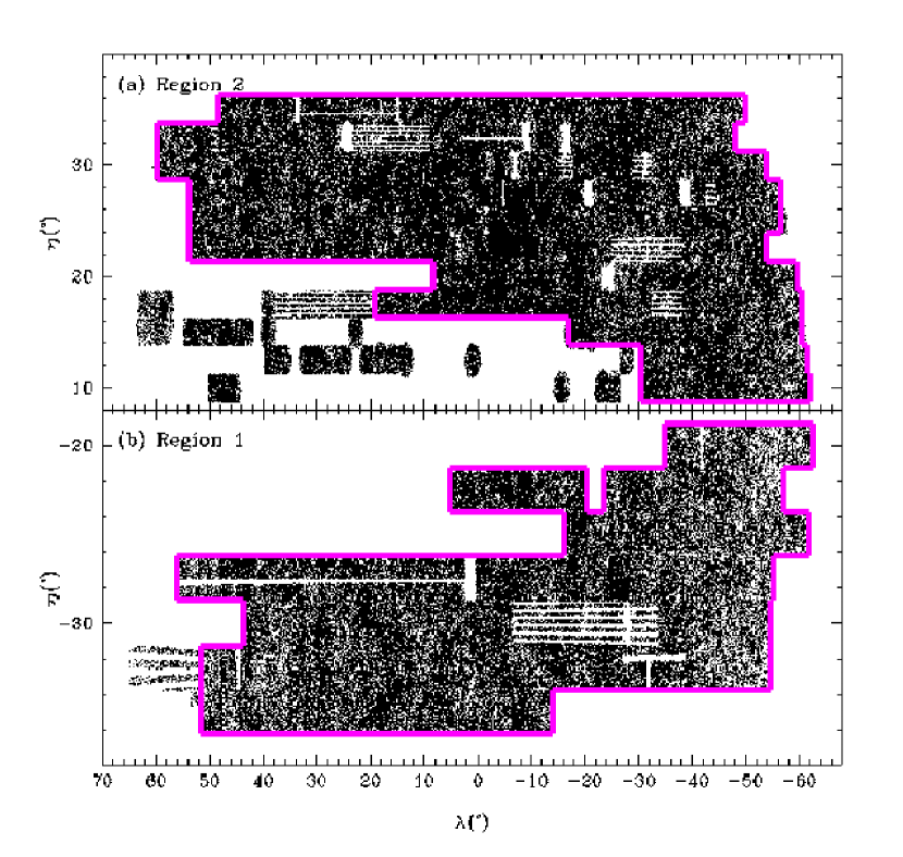
Figure 1.— Angular definition of the SDSS sample used for our topology analysis. Solid lines delineate the boundaries of the analysis regions in the survey coordinate plane $(\lambda,\eta)$.

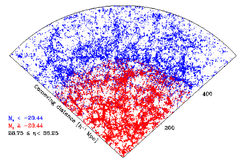
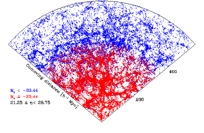
Figure 2.— Distribution of galaxies with $14.5\leq m_{r}\leq 17.5$ in two contiguous $7.5\arcdeg$-thick slices in the analysis region 2. The radial coordinate is Comoving distance and angular coordinate is SDSS survey longitude $\lambda$. [See the electronic edition of the Journal for a color version of this figure. Galaxies brighter and fainter than $M_{*}=-20.44$ are distinguished by color.]

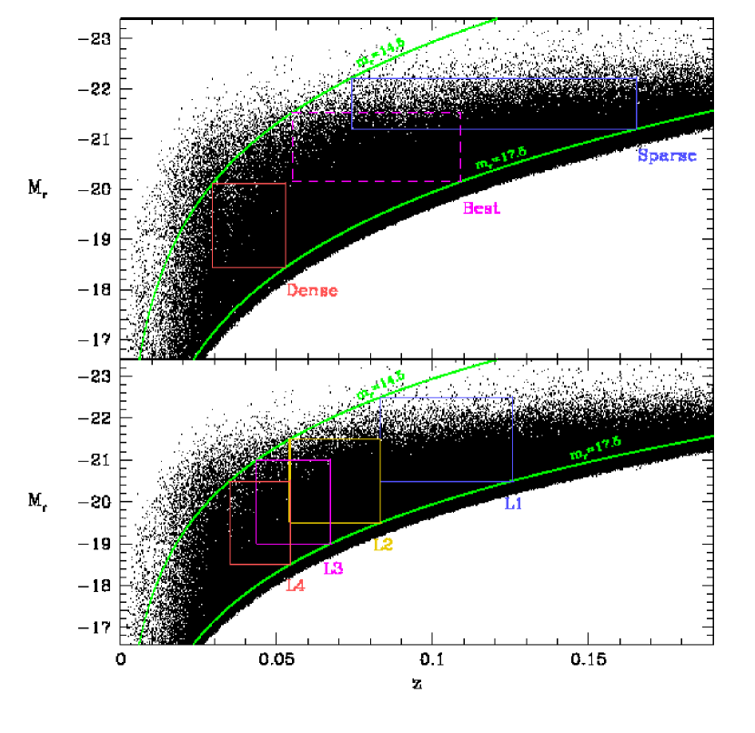
Figure 3.— Sample definitions in the redshift-absolute magnitude space. Top panel shows boundaries of three volume-limited samples used for studying scale dependence of topology. In the bottom panel four samples used for luminosity bias study are defined. The smooth curves delineate the sample boundaries corresponding to our choice of apparent magnitude limits of $14.5\leq m_{r}\leq 17.5$. [See the electronic edition of the Journal for a color version of this figure.]

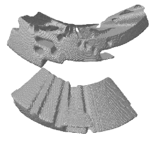
Figure 4.— Three-dimensional views of the mask array looking toward the Earth from the far side after smoothing and trimming. This mask is used for analysis of the Best sample. The upper piece is the region 2, and the lower one is the region 1.

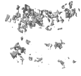
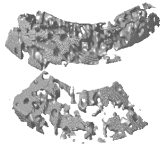
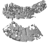
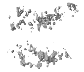
Figure 5.— Three-dimensional view of the galaxy number density field of the Best sample after smoothing and trimming. On the left, density contours enclose low density regions occupying $7\%$ and $50\%$ of the volume, and on the right, contours enclose high density regions filling $50\%$ and $7\%$ of the volume of the Best sample.

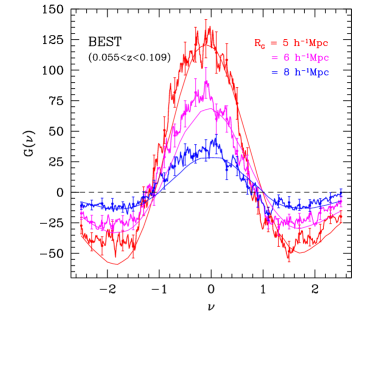
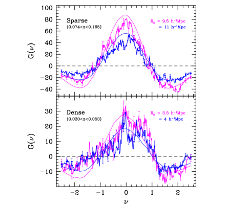
Figure 6.— ($a$) Genus curves measured from the Best sample at three smoothing scales. Solid curves are the genus curves averaged over 100 mock surveys in a $\Lambda{\rm CDM}$ simulation in redshift space at the same smoothing lengths. These curves have not been corrected for systematic uncertainties. ($b$) Similar genus curves for the Sparse and Dense samples and corresponding mock surveys. [See the electronic edition of the Journal for a color version of this figure.]

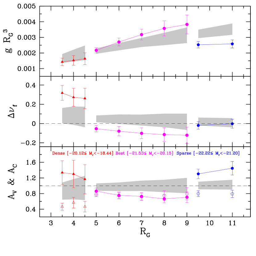
Figure 7.— Genus-related statistics as a function of the Gaussian smoothing length, $R_{G}$. Systematic bias corrections are made by using mock surveys in real space of the $\Lambda{\rm CDM}$ model. Uncertainty limits are derived from mock surveys in redshift space. The shaded areas denote the $1\sigma$ upper and lower limits estimated from the mock samples. In the lower panel, $A_{C}$ is given by filled symbols, $A_{V}$ by open symbols, and the shaded areas are shown only for $A_{C}$. [See the electronic edition of the Journal for a color version of this figure.]

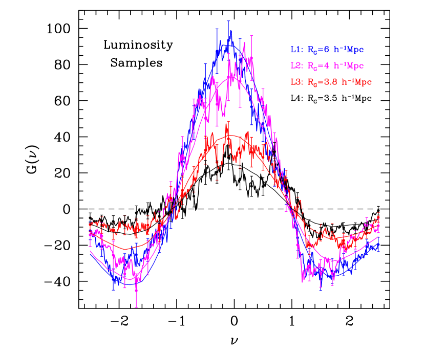
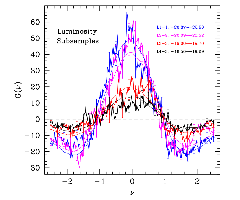
Figure 8.— ($a$) Genus curve calculated by using all galaxies contained in each luminosity sample. Smoothing length is roughly 0.85 times the mean separation between galaxies in each luminosity sample. ($b$) Genus curves of luminosity subsamples which have half the number of galaxies contained in their parent luminosity samples. Only one subsample for each luminosity sample is shown. Smoothing lengths are 7.5, 5.0, 5.0, and 4.4 $\,h^{-1}{\rm Mpc}$ for L1-1, L2-2, L3-3, and L4-3 subsamples, respectively. [See the electronic edition of the Journal for a color version of this figure.]

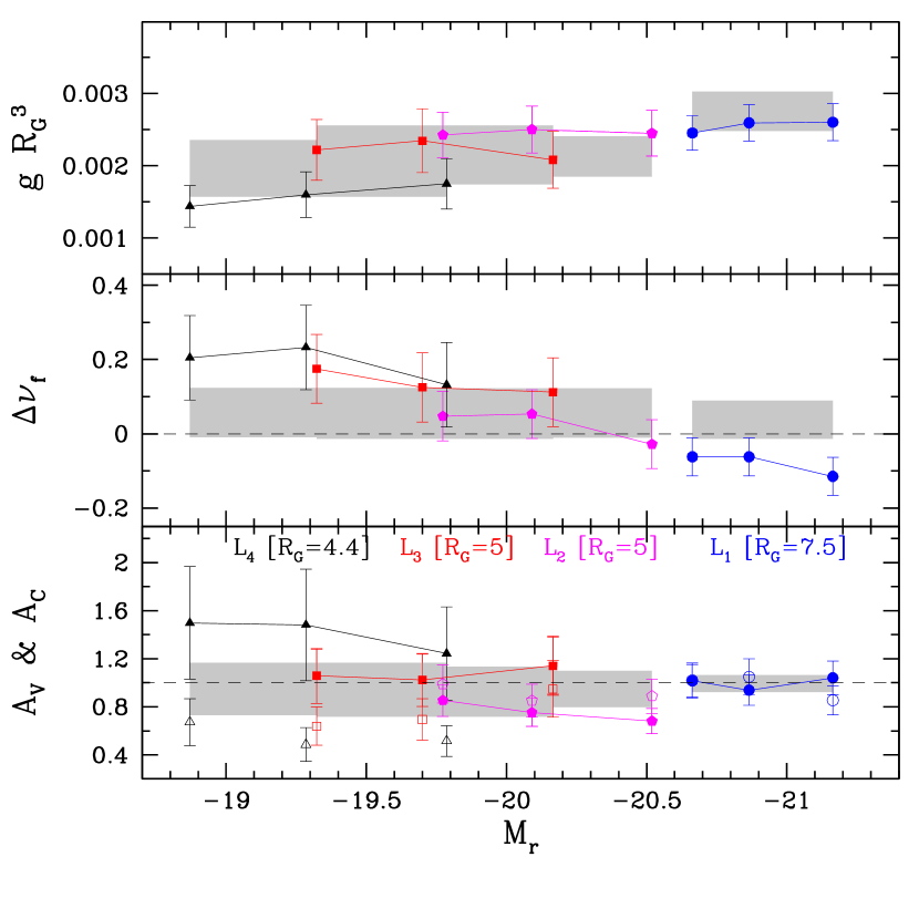
Figure 9.— Genus-related statistics for luminosity subsamples (see Table 1 for definitions). The measured values of subsamples that belong to the same luminosity sample are connected together except for the $A_{V}$ parameter. The smoothing lengths adopted are $R_{G}=$ 7.5, 5.0, 5.0, and 4.4 $\,h^{-1}{\rm Mpc}$ for subsamples of L1, L2, L3, and L4, respectively. Shaded regions are the 1 $\sigma$ variation regions calculated from 100 mock surveys. In the bottom panel, $A_{C}$ is given by filled symbols, $A_{V}$ by open symbols, and the shaded areas are shown only for $A_{C}$. [See the electronic edition of the Journal for a color version of this figure.]

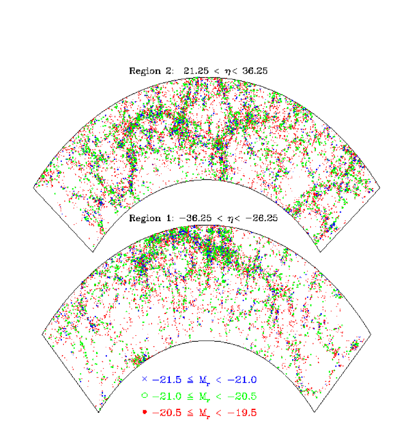
Figure 10.— Distribution of galaxies in the luminosity sample L2 in the comoving distance versus survey longitude coordinate plane projected to the median volume latitude. Galaxies are distinguished by color and point type in accordance with their absolute magnitudes. Crosses are the brightest, circles the middle, and dots the faintest. [See the electronic edition of the Journal for a color version of this figure.]

Table 1Volume-Limited Luminosity and Scale Dependence Samples

Sample Name	Abs. Mag	Redshift	Distance	Galaxies	${N_{\rm res}}\tablenotemark{b}$
Scale Dependence:
Sparse	$-22.22\leq M_{r}<-21.20$	$0.0740<z<0.1654$	$218.2<r<477.1$	$20138$	3618
Best	$-21.53\leq M_{r}<-20.15$	$0.0550<z<0.1091$	$162.9<r<319.0$	$36000$	6466
Dense	$-20.12\leq M_{r}<-18.44$	$0.0295<z<0.0529$	$88.0<r<156.8$	$13011$	2336
Luminosity Dependence:
L1	$-22.50\leq M_{r}<-20.50$	$0.0833<z<0.1257$	$245.1<r<366.1$	$27623$	4961
L1-1	$-22.50\leq M_{r}<-20.87$			13811	2481
L1-2	$-21.16\leq M_{r}<-20.66$			13811	2481
L1-3	$-20.87\leq M_{r}<-20.50$			13811	2481
L2	$-21.50\leq M_{r}<-19.50$	$0.0543<z<0.0833$	$160.9<r<245.1$	$29932$	5374
L2-1	$-21.50\leq M_{r}<-20.09$			14966	2687
L2-2	$-20.52\leq M_{r}<-19.77$			14966	2687
L2-3	$-20.09\leq M_{r}<-19.50$			14966	2687
L3	$-21.00\leq M_{r}<-19.00$	$0.0436<z<0.0674$	$129.6<r<198.9$	$19315$	3468
L3-1	$-21.00\leq M_{r}<-19.70$			9657	1734
L3-2	$-20.17\leq M_{r}<-19.32$			9657	1734
L3-3	$-19.70\leq M_{r}<-19.00$			9657	1734
L4	$-20.50\leq M_{r}<-18.50$	$0.0350<z<0.0543$	$104.1<r<160.9$	$13107$	2353
L4-1	$-20.50\leq M_{r}<-19.29$			6553	1177
L4-2	$-19.76\leq M_{r}<-18.87$			6553	1177
L4-3	$-19.29\leq M_{r}<-18.50$			6553	1177

Note. — The samples are volume-limited with apparent magnitude limits of $14.5\leq m_{r}\leq 17.5$.

Table 2Genus-Related Statistics of the Observational Samples and Subsamples

Sample Name	$\bar{d}$	$R_{\rm G}$	$G_{obs}$	$\Delta\nu$	$A_{\rm V}$	$A_{\rm C}$
Scale Dependence:
Sparse	11.31	9.5	$68.5(56.7){\pm}5.6$	$-0.10(-0.02){\pm}0.04$	$0.72(0.80){\pm}0.07$	$1.29(1.30){\pm}0.12$
		11.0	$41.0(36.0){\pm}4.1$	$-0.06(-0.00){\pm}0.05$	$0.74(0.80){\pm}0.09$	$1.45(1.45){\pm}0.17$
Best	6.14	5.0	$125.4(103.3){\pm}9.7$	$-0.17(-0.05){\pm}0.03$	$0.69(0.78){\pm}0.05$	$0.80(0.86){\pm}0.08$
		6.0	$77.3(69.7){\pm}7.3$	$-0.15(-0.08){\pm}0.05$	$0.71(0.75){\pm}0.07$	$0.74(0.75){\pm}0.08$
		7.0	$52.3(49.8){\pm}5.6$	$-0.15(-0.10){\pm}0.06$	$0.70(0.72){\pm}0.09$	$0.74(0.73){\pm}0.10$
		8.0	$36.2(35.2){\pm}4.9$	$-0.15(-0.11){\pm}0.07$	$0.74(0.75){\pm}0.12$	$0.69(0.66){\pm}0.11$
		9.0	$25.0(24.8){\pm}4.0$	$-0.145(-0.12){\pm}0.08$	$0.79(0.79){\pm}0.16$	$0.74(0.71){\pm}0.14$
Dense	4.17	3.5	$24.1(19.7){\pm}4.1$	$0.18(0.32){\pm}0.078$	$0.42(0.46){\pm}0.08$	$1.21(1.34){\pm}0.28$
		4.0	$15.6(13.6){\pm}3.2$	$0.18(0.27){\pm}0.094$	$0.54(0.57){\pm}0.13$	$1.26(1.30){\pm}0.34$
		4.5	$10.4(9.4){\pm}2.4$	$0.19(0.26){\pm}0.106$	$0.46(0.46){\pm}0.14$	$1.14(1.17){\pm}0.37$
Luminosity Dependence:
L1	7.17	6.0	$85.3(71.8)\pm 7.5$	$-0.11(-0.01)\pm 0.04$	$0.80(0.89)\pm 0.08$	$0.98(1.03)\pm 0.11$
L1-1	9.04	7.5	$47.2(39.3)\pm 4.6$	$-0.14(-0.12)\pm 0.05$	$0.76(0.85)\pm 0.11$	$1.01(1.04)\pm 0.13$
L1-2	9.04	7.5	$47.0(39.2)\pm 4.6$	$-0.09(-0.06)\pm 0.05$	$0.93(1.05)\pm 0.13$	$0.91(0.94)\pm 0.12$
L1-3	9.04	7.5	$44.5(37.1)\pm 4.3$	$-0.09(-0.06)\pm 0.05$	$0.91(1.02)\pm 0.13$	$0.98(1.02)\pm 0.13$
L2	4.71	4.0	$80.8(67.4)\pm 8.6$	$-0.04(0.07)\pm 0.05$	$0.81(0.89)\pm 0.10$	$0.87(0.95)\pm 0.11$
L2-1	5.94	5.0	$46.9(39.2)\pm 6.1$	$-0.13(-0.03)\pm 0.07$	$0.80(0.89)\pm 0.12$	$0.65(0.68)\pm 0.10$
L2-2	5.94	5.0	$47.9(40.0)\pm 6.2$	$-0.05(0.05)\pm 0.07$	$0.77(0.85)\pm 0.12$	$0.72(0.75)\pm 0.11$
L2-3	5.94	5.0	$46.4(38.8)\pm 6.0$	$-0.06(0.05)\pm 0.07$	$0.90(0.99)\pm 0.14$	$0.82(0.85)\pm 0.13$
L3	4.44	3.8	$39.1(33.3)\pm 6.0$	$0.04(0.16)\pm 0.07$	$0.62(0.67)\pm 0.09$	$1.13(1.21)\pm 0.20$
L3-1	5.54	5.0	$19.5(16.5)\pm 3.7$	$0.02(0.11)\pm 0.09$	$0.89(0.95)\pm 0.20$	$1.11(1.14)\pm 0.24$
L3-2	5.54	5.0	$22.0(18.6)\pm 4.1$	$0.03(0.13)\pm 0.09$	$0.65(0.69)\pm 0.15$	$0.99(1.02)\pm 0.22$
L3-3	5.54	5.0	$20.8(17.6)\pm 3.9$	$0.08(0.18)\pm 0.09$	$0.60(0.64)\pm 0.14$	$1.03(1.06)\pm 0.22$
L4	4.09	3.5	$23.3(19.4)\pm 3.9$	$0.12(0.24)\pm 0.09$	$0.44(0.48)\pm 0.09$	$1.23(1.34)\pm 0.31$
L4-1	5.16	4.4	$12.8(10.5)\pm 2.5$	$0.02(0.13)\pm 0.11$	$0.47(0.52)\pm 0.12$	$1.15(1.24)\pm 0.36$
L4-2	5.16	4.4	$11.7(9.6)\pm 2.3$	$0.12(0.23)\pm 0.11$	$0.44(0.49)\pm 0.12$	$1.37(1.48)\pm 0.43$
L4-3	5.16	4.4	$10.5(8.7)\pm 2.1$	$0.09(0.21)\pm 0.11$	$0.61(0.67)\pm 0.16$	$1.38(1.50)\pm 0.43$

Note. — $G_{obs}$ is the amplitude of the observed genus curve, $\Delta\nu$ is shift parameter, and $A_{C}$ and $A_{V}$ are cluster and void abundance parameters, respectively. Uncertainty limits are estimated from mock surveys in redshift space, and systematic bias-corrected values are given in parentheses.

References

- (1) Abazajian, K., et al. 2003, AJ, 126, 2018
- (2) Abazajian, K., et al. 2004, AJ, 128, 502
- (3) Adler, R.J. 1981, The Geometry of Random Fields (Chichester: Wiley)
- (4) Berlind, A. A., & Weinberg, D. H. 2002, ApJ, 575, 587
- (5) Berlind, A. A., Weinberg, D. H., Benson, A. J., Baugh, C. M., Cole, S., Dave, R., Frenk, D. S., Jenkins, A., Katz, N., & Lacey, C. G. 2003, ApJ, 593, 1
- (6) Blanton, M. R., Lin, H., Lupton, R. H., Maley, F. M., Young, N., Zehavi, I., & Loveday, J. 2003a, AJ, 125, 2276
- (7) Blanton, M. R., Brinkmann, J., Csabai, I., Doi, M., Eisenstein, D. J., Fukugita, M., Gunn, J. E., Hogg, D. W., & Schlegel, D. J. 2003b, AJ, 125, 2348
- (8) Blanton, M. R., et al. 2004, submitted to AJ(astro-ph/0410166)
- (9) Canavezes, A., et al. 1998, MNRAS, 297, 777
- (10) Colley, W. N., Gott, J. R., Weinberg, D. H., Park, C., & Berlind, A. A. 2000, ApJ, 529, 795
- (11) Doroshkevich, A.G. 1970, Astrophysics, 6, 320
- (12) Dubinski, J., Kim, J., Park, C., & Humble, R. 2004, New Astronomy, 9, 111
- (13) Eisenstein, D. J., et al. 2001, AJ, 122, 2267
- (14) Fukugita, M., Ichikawa, T., Gunn, J. E., Doi, M., Shimasaku, K., & Schneider, D. P. 1996, AJ, 111, 1748
- (15) Geller, M. J., & Huchra, J. P. 1989, Science, 246, 897
- (16) Gorski, K. M., Davis, M., Strauss, M. A., White, S. D. M. & Yahil, A. 1989, ApJ, 344, 1
- (17) Gott, J. R., Melott, A. L., & Dickinson, M. 1986, ApJ, 306, 341
- (18) Gott, J. R., Cen, R., & Ostriker, J. P. 1996, ApJ, 465, 499
- (19) Gott, J. R., Cen, R., & Ostriker, J. P. 1996, ApJ, 465, 499
- (20) Gott, J. R., Juric, M., Schlegel, D., Hoyle, F., Vogeley, M. S., Tegmark, M., Bahcall, N., & Brinkmann, J. 2003, astro-ph/0310571.
- (21) Gunn, J. E., et al. 1998, AJ, 116, 3040
- (22) Hamilton, A. J. S. & Tegmark, M. 2004, MNRAS, 349, 115
- (23) Hogg, D. W., Finkbeiner, D. P., Schlegel, D. J., & Gunn, J. E. 2001, AJ, 122, 2129
- (24) Hogg, D. W., Baldry, I. K., Blanton, M. R., & Eisenstein, D. J. 2002, astro-ph/0210394
- (25) Hoyle, F., et al. 2002, ApJ, 580, 663
- (26) Hikage, C., et al. 2002, PASJ, 54, 707
- (27) Hikage, C., et al. 2003, PASJ, 55, 911
- (28) Jing, Y. P., & Börner, G. 2004, ApJ, 607, 140
- (29) Kayo, I., et al. 2004, PASJ, 56, 415
- (30) Kravtsov, A. V., Berlind, A. A., Wechsler, R. H., Klypin, A. A., Gottlober, S., Allgood, B., & Primack, J. R. 2004, ApJ, 609, 35
- (31) La, D., & Steinhardt, P. J. 1989, Phys. Rev. Lett., 62,376
- (32) Lupton, R. H., Gunn, J. E., Ivezic, Z., Knapp, G. R., Kent, S., & Yasuda, N. 2001, in ASP Conf. Ser. 238, Astronomical Data Analysis Software and Systems X, ed. F. R. Harnden, Jr., F. A. Primini, & H. E. Payne (San Francisco: ASP), 269
- (33) Ma, C., & Fry, J. N. 2000, ApJ, 543, 503
- (34) Matsubara, T. 1994, ApJ, 434, L43
- (35) Melott, A. L., Weinberg, D. H., & Gott, J. R. 1988, ApJ, 328, 50
- (36) Norberg, P., et al. 2001, MNRAS, 328, 64
- (37) Park, C., & Gott, J. R. 1991, ApJ, 378, 457
- (38) Park, C., Gott, J. R., Melott, A. L., & Karachentsev, I. D. 1992, ApJ, 387, 1
- (39) Park, C., Vogeley, M. S., Geller, J., & Huchra, J. P. 1994, ApJ, 431,569
- (40) Park, C., Gott, J. R.,& Choi, Y. 2001, ApJ, 553, 33
- (41) Park, C., Kim, J., & Gott, J. R. 2005, in preparation
- (42) Pier, J. R., Munn, J. A., Hindsley, R. B., Hennessy, G. S., Kent, S. M., Lupton, R. H., & Ivezic, R. 2003, AJ, 125, 1559
- (43) Richards, G. T., et al. 2002, AJ, 123, 2945
- (44) Protogeros, Z. A. M., & Weinberg, D. H. 1997, ApJ, 489, 457
- (45) Schlegel, D. J., Finkbeiner, D. P., & Davis, M. 1998, ApJ, 500, 525
- (46) Spergel, D. N., et al. 2003, ApJS, 148, 175
- (47) Smith, J. A., et al. 2002, AJ, 123, 2121
- (48) Stoughton, C., et al. 2002, AJ, 123, 485
- (49) Strauss, M. A., et al. 2002, AJ, 124, 1810
- (50) Tegmark, M., et al. 2004, ApJ, 606, 702
- (51) Vogeley, M. S., Park, C., Geller, M. J., Huchra, J. P., & Gott, J. R. 1994, ApJ, 420,525
- (52) Weinberg, D. H., Gott, J. R., & Melott, A. L. 1987, ApJ, 321, 2
- (53) Weinberg, D. M. 1988, PASP, 100, 1373
- (54) York, D., et al. 2000, AJ, 120, 1579
- (55) Zehavi, I., et al. 2004, submitted to ApJ(astro-ph/0408569)
- (56) Zheng, Z., Berlind, A. A., Weinberg, D. H., Benson, A. J., Baugh, C. M., Cole, S., Dave, R., Frenk, C. S., Katz, N., & Lacey, C. G. 2004, submitted to ApJ(astro-ph/0408564)