Observational constraints on low redshift evolution of dark energy: How consistent are different observations?

Abstract

The dark energy component of the universe is often interpreted either in terms of a cosmological constant or as a scalar field. A generic feature of the scalar field models is that the equation of state parameter $w\equiv P/\rho$ for the dark energy need not satisfy $w=-1$ and, in general, it can be a function of time. Using the Markov chain Monte Carlo method we perform a critical analysis of the cosmological parameter space, allowing for a varying $w$. We use constraints on $w(z)$ from the observations of high redshift supernovae (SN), the WMAP observations of CMB anisotropies and abundance of rich clusters of galaxies. For models with a constant $w$, the $\Lambda$CDM model is allowed with a probability of about $6\%$ by the SN observations while it is allowed with a probability of $98.9\%$ by WMAP observations. The $\Lambda$CDM model is allowed even within the context of models with variable $w$: WMAP observations allow it with a probability of $99.1\%$ whereas SN data allows it with $23\%$ probability. The SN data, on its own, favors phantom like equation of state ($w<-1$) and high values for $\Omega_{NR}$. It does not distinguish between constant $w$ (with $w<-1$) models and those with varying $w(z)$ in a statistically significant manner. The SN data allows a very wide range for variation of dark energy density, e.g., a variation by factor ten in the dark energy density between $z=0$ and $z=1$ is allowed at $95\%$ confidence level. WMAP observations provide a better constraint and the corresponding allowed variation is less than a factor of three. Allowing for variation in $w$ has an impact on the values for other cosmological parameters in that the allowed range often becomes larger. There is significant tension between SN and WMAP observations; the best fit model for one is often ruled out by the other at a very high confidence limit. Hence results based on only one of these can lead to unreliable conclusions. Given the divergence in models favored by individual observations, and the fact that the best fit models are ruled out in the combined analysis, there is a distinct possibility of the existence of systematic errors which are not understood.

I Introduction

Observational evidence for accelerated expansion in the universe has been growing in the last two decades crisis2 . Observations of high redshift supernovae nova_data1 ; nova_data3 provided an independent confirmation. Using these along with observations of cosmic microwave background radiation (CMB) boomerang ; wmap_params and large scale structure 2df ; sdss , we can construct a “concordance” model for cosmology and study variations around it (e.g., see wmap_params ; 2003Sci…299.1532B ; 2004PhRvD..69j3501T ; for an overview of our current understanding, see TPabhay ).

Observations indicate that dark energy should have an equation of state parameter $w\equiv P/\rho<-1/3$ for the universe to undergo accelerated expansion. Indeed, observations show that dark energy is the dominant component of our universe. The cosmological constant is the simplest explanation for accelerated expansion ccprob ; review3 and it is known to be consistent with observations. In order to avoid theoretical problems related to cosmological constant ccprob , other scenarios have been investigated. In these models one can have $w\neq-1$ and in general $w$ varies with redshift. These models include quintessence quint1 , k-essence 2001PhRvD..63j3510A , tachyons tachyon1 ; 2003PhRvD..67f3504B , phantom fields 2002PhLB..545…23C , branes brane1 , etc. There are also some phenomenological models water , field theoretical and renormalisation group based models (see e.g. tp173 ), models that unify dark matter and dark energy unified_dedm1 and many others like those based on horizon thermodynamics (e.g. see 2005astro.ph..5133S ). Even though these models have been proposed to overcome the fine tuning problem for cosmological constant, most of these require similar fine tuning of parameter(s) to be consistent with observations. Nevertheless, they raise the possibility of $w(z)$ evolving with time (or being different from $-1$), which — in principle — can be tested by observations.

Given that $w<-1/3$ for dark energy for the universe to undergo accelerated expansion, the energy density of this component changes at a much slower rate than that of matter and radiation. Indeed, $w=-1$ for cosmological constant and in this case the energy density is a constant. Unless $w$ is a rapidly varying function of redshift and becomes $w\sim 0$ at ($z\leq 1$), the energy density of the dark energy component should be negligible at high redshifts ($z\gg 1$) as compared to that of non-relativistic matter. If dark energy evolves in a manner such that its energy density is comparable to, or greater than the matter density in the universe at high redshifts then the basic structure of the cosmological model needs to be modified. We do not consider such models here. We confine our attention to models with dark energy density being an insignificant component of the universe at $z\gg 1$ and choose observations which are sensitive to evolution of $w(z)$ at redshifts $z\lesssim 1$.

To put the present work in context, we recall that combining supernova observations with the WMAP data provides strong constraints on the variation of dark energy density 2005MNRAS.356L..11J . (A review of relevant observations for constraining dark energy models along with a summary of the previous work in this area is given in Section II.2.) Reproducing the location of acoustic features requires the angular diameter distance to the last scattering surface to be in the correct range. This analysis showed that while the data from SN observations allows for a large range in parameters of dark energy, combining with WMAP data limits this range significantly. However, in that work, we did not explore the cosmological parameter space widely and had fixed nearly all parameters other than those used to describe evolution of dark energy. In the present work, we allow many cosmological parameters to vary and include constraints from cluster abundance in addition to the supernova and WMAP constraints.

In addition to obtaining quantitative bounds on parameters in different contexts, we address the following key issues in this paper:

• Does allowing cosmological parameters to vary weaken the constraints on variation of dark energy?

• Conversely, how does the allowed range for different cosmological parameters change when we allow for a epoch dependent $w(z)$ ?

• Do the observational constraints agree with each other? In particular, what kind of cosmological models are preferred by SN and WMAP observations individually ?

The last point is important and requires elaboration. Different observational sets are combined together precisely because these observations are sensitive to different combinations of cosmological parameters and facilitate in breaking degeneracies between parameters. If we consider $\Lambda$CDM models then the SN observations, for example, broadly depend on the combination ($0.85\Omega_{NR}-0.53\Omega_{V}$) 2005A&A…429..807C while WMAP is sensitive to ($\Omega_{NR}+\Omega_{V})$ wmap_params , a feature which was originally highlighted in the literature as ‘cosmic complementarity’. Therefore, we cannot expect constraints from different observations to agree over the entire parameter space. At the same time, we do not expect models favored by one observation to be ruled out by another when such a divergence is not expected. This divergence may point to some shortcomings in the model, or to systematic errors in observations, or even to an incorrect choice of priors. If all observational sets are consistent then we should be able to derive similar constraints using subsets of observations, even though the final constraints may not be as tight as with the full set of observations.

In order to address the questions listed above in a systematic manner, we proceed in three steps. We choose a ‘base’ reference model with cold dark matter and cosmological constant, with neutrinos contributing a negligible amount to the energy density of the Universe. We assume that the Universe is flat and restrict ourselves to an unbroken power law for the primordial power spectrum of density fluctuations and we assume that the perturbations are adiabatic. Another assumption is that the perturbations in tensor mode are negligible and we take $r=0$ 2005PhRvD..71j3515S . We choose this to be our standard model as this can be described by a compact set of parameters.

Next, we generalize from $\Lambda$CDM models ($w=-1$) to study a wider class of dark energy models with a constant $w$ and address the issues listed above. In this case, we also study the effect of perturbations in dark energy. Finally, we generalize to models in which $w$ is allowed to vary with $z$ in a parameterized form. This approach allows us to delineate changes that come about from choosing a constant $w\neq-1$, from those allowed by a varying dark energy. We do not impose theoretically motivated constraints on models, e.g. we do not require $w\geq-1$ as the present work is focused on understanding the nature of models favored by observations.

The paper is organized as follows: In section II we discuss the background cosmological equations followed by a brief review on the various observation used to constrain dark energy equation of state and the observations we concentrate on. The Markov Chain Monte Carlo method is discussed in section III and detailed results are presented in section IV. We conclude with a discussion of the results and future prospects for constraining dark energy models in section V.

II Theoretical background

II.1 Cosmological equations

If we assume that each of the constituents of the homogeneous and isotropic universe can be considered to be an ideal fluid, and that the space is flat, the Friedman equations become:

$$\left(\frac{\dot{a}}{a}\right)^{2} = \frac{8\pi G}{3}\rho$$ (1)

$$\frac{\ddot{a}}{a} = -\frac{4\pi G}{3}(\rho+3P)$$ (2)

where $P$ is the pressure and $\rho=\rho_{NR}+\rho_{\gamma}+\rho_{{}_{\rm DE}}$ with the respective terms denoting energy densities for nonrelativistic matter, for radiation/relativistic matter and for dark energy. Pressure is zero for the non-relativistic component, whereas radiation and relativistic matter have $P_{\gamma}=\rho_{\gamma}/3$. If the cosmological constant is the source of acceleration then $\rho_{{}_{\rm DE}}=$ constant and $P_{{}_{\rm DE}}=-\rho_{{}_{\rm DE}}$.

An obvious generalization is to consider models with a constant equation of state parameter $w\equiv P/\rho=$ constant. One can, in fact, further generalize to models with a varying equation of state parameter $w(z)$. Since a function is equivalent to an infinite set of numbers (defined e.g. by a Taylor-Laurent series coefficients), it is clearly not possible to constrain the form of an arbitrary function $w(z)$ using finite number of observations. One possible way of circumventing this issue is to parameterize the function $w(z)$ by a finite number of parameters and try to constrain these parameters by observations. There have been many attempts to describe varying dark energy with different parameterizations constraints_2 ; 2004ApJ…617L…1B ; 2005MNRAS.356L..11J ; constraints_10 ; holographic ; Hannestad:2004cb where the functional form of $w(z)$ is fixed and the variation is described with a small number of parameters. Observational constraints depend on the specific parameterization chosen, but it should be possible to glean some parameterization independent results from the analysis.

To model varying dark energy we use two parameterizations

$$w(z)=w_{0}+w^{\prime}(z=0)\frac{z}{(1+z)^{p}}~{};~{}~{}~{}~{}~{}~{}~{}~{}p=1,~{}2$$ (3)

These are chosen so that, among other things, the high redshift behavior is completely different in these two parameterizations 2005MNRAS.356L..11J . If $p=1$ p1 , the asymptotic value $w(\infty)=w_{0}+w^{\prime}(z=0)$ and for $p=2$, $w(\infty)=w_{0}$. For both $p=1,2$, the present value $w(0)=w_{0}$. Clearly, we must have $w(z\gg 1)\leq-1/3$ for the standard cosmological models with a hot big bang to be valid. This restriction is imposed over and above the priors used in our study.

Integrating $d(\rho a^{3})=-w(z)\rho da^{3}$, the energy density can be expressed as

$$\frac{\rho_{{}_{DE}}}{\rho_{{}_{DE_{0}}}}=\left(1+z\right)^{3\left(1+w_{0}+w^{\prime}_{0}\right)}\exp{\left[-\frac{3w^{\prime}_{0})z}{1+z}\right]}$$ (4)

for $p=1$ (in Eq. 3) and

$$\frac{\rho_{{}_{DE}}}{\rho_{{}_{DE_{0}}}}=\left(1+z\right)^{3\left(1+w_{0}\right)}\exp{\left[\frac{3w^{\prime}_{0}}{2}\left(\frac{z}{1+z}\right)^{2}\right]}$$ (5)

for $p=2$. The allowed range of parameters $w_{0}$ and $w^{\prime}_{0}\equiv w^{\prime}(z=0)$ is likely to be different for different $p$. However, the allowed variation at low redshifts in $\rho_{{}_{DE}}$ should be similar in both models as observations actually probe the variation of dark energy density. Indeed, in an earlier study 2005MNRAS.356L..11J where we had studied a restricted class of models, we found this to be the case. For example, $\rho_{{}_{DE}}$ can vary by at most a factor two up to $z=2$ when both the WMAP and SN data are taken into account 2005MNRAS.356L..11J . This reaffirms the expectation that the results are parameterization independent at some level.

II.2 Observational constraints

In this subsection, we briefly review potential observational constraints on dark energy and we also summarize previous work in this area.

Constraints on dark energy models essentially arise as follows: To begin with, dark energy affects the rate of expansion of the universe and thus the luminosity distance and also the angular diameter distance. Constraints from observations of high redshift supernovae 1998ApJ…509…74G ; nova_data1 ; dynamic_de1 ; 2005A&A…429..807C ; 2004MNRAS.354..275A ; dynamic_de5 and the location of peaks in the angular power spectrum of CMB anisotropies mainly use this feature 2004PhRvD..70j3523E . The signature of acoustic peaks in correlation function of galaxies also provides a similar geometric constraint 2005astro.ph..1171E . There is also an effect on weak lensing statistics through changes in distance-redshift relation 2002PhRvD..65f3001H ; 2003ApJ…583..566M ; 2003MNRAS.341..251W ; 2003PhRvL..91d1301A ; 2003PhRvL..91n1302J .

Second, the rate of expansion influences the growth of perturbations in the universe and this leads to another set of probes of dark energy 2001PhRvD..64h3501B . Abundance of rich clusters of galaxies, their evolution and the integrated Sachs-Wolfe (ISW) effect belong to this category of constraints, along with constraints from redshift space distortions 1999ApJ…517…40B ; cluster2 ; cluster4 ; 2004astro.ph..8252V ; 2004astro.ph..9207Y ; Calvao:2002zr . All these constraints are sensitive to different aspects of dark energy and a combination of all of these can put tight limits on models. The redshift space distortions are a local effect as these are sensitive to the rate of growth of density perturbations at a given epoch. The abundance of rich clusters of galaxies, the ISW effect and distances are integrated effects in that the effect of dark energy is averaged over a range of redshifts in some sense.

Observations of high redshift supernovae of type Ia provide the most unambiguous evidence for accelerated expansion 1998ApJ…509…74G ; nova_data1 ; dynamic_de1 ; 2005A&A…429..807C ; 2004MNRAS.354..275A . Assuming these sources to be standard candles, observations spanning a range of redshifts can be used to study the change in rate of expansion and this imposes direct constraints on the variation of dark energy density. Supernovae have been observed up to a redshift of $z_{max}\simeq 1.8$ and hence can be used to constrain models of dark energy up to this redshift. Constraints from SN observations alone however, permit a large variation in the dark energy parameters 2004MNRAS.354..275A and in particular favor models with $w<-1$ at the present epoch nova_data3 ; dynamic_de1 ; 2005A&A…429..807C .

Baryon oscillations in the matter-radiation fluid prior to decoupling provide a standard scale and the angle at which the acoustic peaks occur in the angular power spectrum of temperature anisotropies in the CMB fixes the distance to the surface of last scattering. This provides a useful constraint on models of dark energy 2004PhRvD..70j3523E as long as dark energy does not affect the dynamics of universe at the time of decoupling of matter and radiation. Unlike supernovae that are observed over a range of redshifts where dark energy is dominant, the surface of last scattering is at $z\simeq 1100$. However, the exquisite quality of CMB anisotropy measurements makes this a very useful constraint and these observations offer a constraint that is different from SN observations 2005MNRAS.356L..11J . Indeed, as we shall see, WMAP and SN observations often favor models that are mutually unacceptable.

Recent detection of the baryon acoustic peak in galaxy correlation function using the luminous red galaxy sample of the SDSS survey has provided an additional handle to constrain cosmological parameters 2005astro.ph..1171E . The geometric constraint from these observations can, in principle, constrain models of dark energy. A measurement of the angular scale corresponding to the peak at different redshifts can indeed be a powerful constraint.

If we consider a given cosmological model that is consistent with observations of CMB anisotropy then the amplitude of fluctuations at the time of decoupling is fixed, and its linearly extrapolated value today can be computed using linear perturbation theory. The abundance of rich clusters of galaxies is related to the amplitude of perturbations in dark matter at a scale of about $8$h^-1Mpc. If we study different models for dark energy while other parameters are not changed, the abundance of rich clusters constrains the net growth of structures between the epoch of decoupling and the present epoch lss_de .

Redshift space distortions due to kinematics and the Alcock-Paczynski effect are also potential probes of dark energy 1979Natur.281..358A ; 2004astro.ph..9207Y . Ongoing surveys like the SDSS and future surveys will be able to distinguish between different dark energy models through these effects 2003NewAR..47..775W . However, this method does not provide useful constraints at present.

Dependence of the distance-redshift relation and a different rate of growth for perturbations, as well as changes in the matter power spectrum are also reflected in weak lensing statistics. Several studies have been carried out on the potential constraints that can be put on dark energy models from weak lensing observations and their degeneracy with other parameters. These studies indicate that future surveys will be able to put strong constraints on dark energy models 2003ApJ…583..566M ; 2003PhRvL..91d1301A .

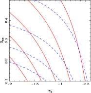
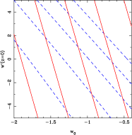
Figure 1: The left figure in this panel shows contours of constant luminosity distance $H_{0}D_{L}(z)/c$ in $\Omega_{NR}-w$ plane. The red/solid contours are for luminosity distance at redshift $z=0.17$ and blue/dashed ones are for luminosity distance at redshift $z=1.17$. The red/solid contours from top right to bottom left correspond to values between $H_{0}D_{L}(z=0.17)/c=0.19-0.21$ and blue/dashed lines are for $H_{0}D_{L}(z=1.17)/c=1.52-2.45$. The other plots show contours in the $w_{0}-w^{\prime}(z=0)$ plane. The second figure shows contours of constant $H_{0}D_{L}(z=0.17)/c$ and $H_{0}D_{L}(z=1.17)/c$. Starting from upper right the contours are for $H_{0}D_{L}(z=0.17)/c=0.18-0.2$ and $H_{0}D_{L}(z=1.17)/c=1.63-2.1$. The third panel shows contours of redshift at which the expansion of the universe starts to accelerate. Starting from upper right corner in counter-clockwise direction, the contours are for $z=0$, $0.2$, 0$.4$, $0.6$ and $0.8$. The constraint from SN observations essentially constrains this redshift and hence the allowed region can be expected to follow these contours. The next panel shows red-shift at which the energy density in matter and dark energy are equal. The curves, starting from left are for $z=0.2$, $0.4$, $0.6$, $0.8$ and $1.0$. Structure formation constraints are likely to follow these contours as the rate of growth for density perturbations is significant only in the matter dominated era. The right panel shows contours of $w_{eff}$ at the surface of last scattering (see Eq. 8). From top right towards bottom left the values are $w_{eff}=-0.5$, $-1.0$, $-1.5$ and $-2.0$ If the location of acoustic peaks provides the main constraint then the region allowed by CMB observations should follow these contours. We have used $\Omega_{NR}=0.3$ for these plots.

Growth of perturbations also leaves a signature in the CMB anisotropy spectrum at large angular scales. The ISW effect leads to an enhancement in the angular power spectrum at these scales. The detailed form of this enhancement depends on the equation of state parameter $w$ and its variation. This effect can be detected by cross-correlation of temperature anisotropies with the foreground distribution of matter isw0 . It is difficult to distinguish the ISW effect from the effect of a small but non-zero optical depth $\tau$ due to re-ionisation by using only the temperature anisotropies in the CMB, cross-correlation with the matter distribution or polarization anisotropies in the CMB must be used.

Redshift surveys of galaxy clustering do not constrain properties of dark energy directly, however the shape of the power spectrum constrains the combination $\Gamma=\Omega_{NR}h$ 1992MNRAS.258P…1E . This provides an indirect constraint on dark energy through the well known degeneracy between $\Omega_{NR}$ and $w_{0}$ (e.g. see 2005MNRAS.356L..11J ).

The large number of different observations that can be used to constrain dark energy models is encouraging. Indeed, many attempts have been made to use some of these observations to put constraints on models lss_de ; 2004PhRvD..69j3501T ; 2005MNRAS.356L..11J ; constraints_2 ; constraints_3 .

II.3 A choice of three observations

In this work, we concentrate on SN, WMAP and cluster abundance observations. We briefly explain the reason for this choice and the kind of constraints one can expect.

The left panel in Fig. 1 shows the degeneracy in $\Omega_{NR}$ and $w_{0}$ (for models with constant $w$; i.e., with $w^{\prime}_{0}=0$ in Eq. 3). The figure shows contours of constant luminosity distance $H_{0}d_{l}(z)$ at $z=0.17$ (red/solid curves) and $z=1.17$ (blue/dashed curves). The second panel displays the constant luminosity distance contours in the $w^{\prime}(z=0)-w_{0}$ plane for $p=2$ if $\Omega_{NR}=0.3$. Given that SN observations constrain luminosity distance as a function of redshifts, these figures illustrate the shape of the allowed region that we are likely to get and also demonstrates the degeneracies between different parameters. The third panel shows how the redshift at which the expansion of the universe begins to accelerate depends on the parameters $w_{0}$ and $w^{\prime}(z=0)$ for $p=2$. This epoch is constrained by SN observations and hence the allowed region in parameter space should lie between contours of this nature. Clearly, regions with a late onset of acceleration (upper right corner) as well as a very early onset of acceleration (lower right corner) will be ruled out by observations of supernovae.

The fourth panel of this figure shows the redshift at which matter and dark energy contribute equally in terms of the energy density of the universe. Structure formation constraints are likely to follow these contours as the rate of growth for density perturbations is significant only in the matter dominated era. Too little structure formation (upper right corner) as well as too much structure formation (lower left corner) are likely to restrict the allowed models along a diagonal (upper left to lower right) in this plane.

Lastly, the location of acoustic peaks in the angular power spectrum of temperature anisotropies in the CMB is the most significant constraint provided by CMB observations. This essentially constrains the distance to the surface of last scattering and hence a suitably defined (see eqn.(8)) mean value ($w_{eff}$) for $w$. The right panel shows contours of $w_{eff}$, which run almost diagonal in this plane. Thus a band of allowed models is the likely outcome of comparison with observations. The contours of $w_{eff}$ are the same as contours of equal distance to the surface of last scattering, or the $l$ corresponding to the first peak in the angular power spectrum of CMB temperature fluctuations.

SN data provides geometric constraints for dark energy evolution. These constraints are obtained by comparing the predicted luminosity distance to the SN with the observed one. The theoretical model and observations are compared for luminosity measured in magnitudes:

$$m_{B}(z)={\mathcal{M}}+5log_{10}(D_{L})$$ (6)

where ${\mathcal{M}}=M-5log_{10}(H_{0})$ and $D_{L}=H_{0}d_{L}$, $M$ being the absolute magnitude of the object and $d_{L}$ is the luminosity distance

$$d_{L}=(1+z)a(t_{0})r(z);~{}~{}~{}~{}r(z)=c\int\frac{dz}{(1+z)~{}H(z)}$$ (7)

where $z$ is the redshift. This depends on evolution of dark energy through $H(z)$. For our analysis we use the combined gold and silver SN data set in nova_data3 . This data is a collection of supernova observations from nova_data1 ; 1998ApJ…509…74G and many other sources with $16$ supernovae discovered with Hubble space telescope nova_data3 . The parameter space for comparison of models with SN observations is small and we do a dense sampling of the parameter space.

CMB anisotropies constrain dark energy in two ways, through the distance to the last scattering surface and through the ISW effect. Given that the physics of recombination and evolution of perturbations does not change if $w(z)$ remains within some safe limits, any change in the location of peaks will be due to dark energy 2004PhRvD..70j3523E . The angular size $\theta$ of the Hubble radius at the time of decoupling can be written as:

$$\theta^{-1} = \frac{H(z)/H_{0}}{\int\limits_{0}^{z}{dy}/{\left(H(y)/H_{0}\right)}}$$ (8)

$$\simeq \frac{\sqrt{\Omega_{NR}\left(1+z\right)^{3}}}{\int\limits_{0}^{z}{dy}/{\sqrt{\Omega_{NR}\left(1+z\right)^{3}+\varrho^{DE}(z)/\varrho^{DE}_{0}}}}$$

$$\equiv \frac{\sqrt{\Omega_{NR}\left(1+z\right)^{3}}}{\int\limits_{0}^{z}{dy}/{\sqrt{\Omega_{NR}\left(1+z\right)^{3}+\Omega_{de}\left(1+z\right)^{3\left(1+w_{eff}\right)}}}}.$$

The second line is obtained as decoupling happens at a redshift where dark energy is not important, and if we ignore the contribution of radiation and relativistic matter; the last equation defines $w_{eff}$. Clearly, the value of the integral will be different if we change $w_{0}$, $w^{\prime}(z=0)$ and there will also be some dependence on the parameterized form. Location of peaks in the angular power spectrum of the CMB provide a constraint, but this can only constrain $w_{eff}$ and not all of $w_{0}$, $w^{\prime}(z=0)$ and $p$. Therefore if the present value $w_{0}<w_{eff}$ then it is essential that $w^{\prime}(z=0)>0$, and similarly if $w_{0}>w_{eff}$ then $w^{\prime}(z=0)<0$ is needed to ensure that the integrals match. Specifically, the combination of $w_{0}$, $w^{\prime}(z=0)$ and $p$ should give us a $w_{eff}$ within the allowed range.

In our analysis, we use the angular power spectrum of the CMB temperature anisotropies cmbrev1 ; White and Cohn (2002) as observed by WMAP and these are compared to theoretical predictions using the likelihood program provided by the WMAP team wmap_lik . We vary the amplitude of the spectrum till we get the best fit with WMAP observations. Note that this is different from the commonly used approach of normalizing the angular power spectrum at $l=10$. As we use the entire angular power spectrum for comparison with observations, the impact of ISW effect on the likelihood is relatively small.

It has been pointed out that constraints from structure formation restrict the allowed variation of dark energy in a significant manner lss_de . We use observed abundance of rich clusters 1999ApJ…517…40B ; cluster2 ; cluster4 to apply this constraint. Since the mass of a typical rich cluster corresponds to the scale of $8$h^-1Mpc, cluster abundance observations therefore constrain $\sigma_{8}$, the rms fluctuations in density contrast at $8$h^-1Mpc. The number density of clusters depends strongly on $\sigma_{8}$ and $\Omega_{NR}$. We use the $\sigma_{8}$ constraints given in 1999ApJ…517…40B from ROSAT deep cluster survey and are given by $\sigma_{8}=(0.58\pm 0.1)\times\Omega_{NR}^{-0.47+0.16\Omega_{NR}}$ at $99\%$ confidence level. The cosmological model should predict $\sigma_{8}$ in the allowed range in order to be consistent with observations.

Recent detection of the baryon acoustic peak using luminous red galaxy sample of the SDSS survey has provided an additional handle to constrain the cosmological parameters 2005astro.ph..1171E . We also used distance scale $D_{V}$ at redshift $z=0.35$ introduced in the above reference to further constrain the cosmological models. Here $D_{V}(0.35)^{3}\equiv D_{M}(z)^{2}cz/H(z)$ and the observational constraint is $D_{V}(0.35)=1370\pm 64~{}~{}Mpc$ at the $1\sigma$ level. This fourth observation does not add significantly to other constraints listed here and we will not describe quantitative results from this constraint here.

Priors used in the present study are listed in Table 1. Apart from these limits on the models studied here, we also assumed that neutrinos are massless and the ratio $r$ of tensor to scalar mode is zero. These assumptions are consistent with the known upper bounds, and in any case these do not make any difference to the observations used here as constraints 2005PhRvD..71j3515S .

Table 1: This table lists the priors used in the present work. Apart from the range of parameters listed in the table, we assumed that the universe is flat. We assumed that the primordial power spectrum had a constant index. Further, we ignored the effect of tensor perturbations. The range of values for $w_{0}$ and $w^{\prime}(z=0)$ is as given below, but with the constraint that $w(z=1000)\leq-1/3$. Any combination of $w_{0}$ and $w^{\prime}(z=0)$ that did not satisfy this constraint was not considered.

Parameter	Lower limit	Upper limit
$\Omega_{B}$	$0.03$	$0.06$
$\Omega_{NR}$	$0.1$	$0.5$
$h$	$0.6$	$0.8$
$\tau$	$0.0$	$0.4$
$n$	$0.86$	$1.10$
$w_{0}$	$-2.0$	$-0.4$
$w^{\prime}(z=0)$	$-5.0$	$5.0$

III Markov chain monte Carlo method

We compute $\chi^{2}$ using the routines provided by the WMAP team wmap_lik . The CMBFAST package 1996ApJ…469..437S is used for computing the theoretical angular power spectrum for a given set of cosmological parameters. We have combined the likelihood program with the CMBFAST code and this required a few minor changes in the CMBFAST driver routine. Given the large number of parameters, the task of finding the minimum $\chi^{2}$ and mapping its behavior in the entire range of values for parameters is computationally intensive.

We adapt the Metropolis algorithm metropolis (also known in the context of parameter estimation as the Markov Chain Monte Carlo (MCMC) method wmap_lik ; mcmc2 ) for efficiently mapping regions with low values of $\chi^{2}$. The algorithm used is as follows:

1. Start from a random point ${\mathbf{r}}_{i}$ in parameter space and compute $C_{l}$ and $\chi^{2}({\mathbf{r}}_{i})$.

2. Consider a small random displacement ${\mathbf{r}}_{i+1}={\mathbf{r}}_{i}+d{\mathbf{r}}$ and compute $\chi^{2}({\mathbf{r}}_{i+1})$.

3. If $\chi^{2}({\mathbf{r}}_{i+1})\leq\chi^{2}({\mathbf{r}}_{i})$ then $i\rightarrow i+1$. Go to the first step.

4. Else:

   • Compute $\Delta\chi^{2}=\chi^{2}({\mathbf{r}}_{i+1})-\chi^{2}({\mathbf{r}}_{i})$ and $\exp[-\alpha~{}\Delta\chi^{2}]$.

   • Compare this with a random number $0\leq\beta\leq 1$.

   • If $\beta\leq\exp[-\alpha~{}\Delta\chi^{2}]$ then $i\rightarrow i+1$. Go to the first step.

The size of the small displacement $d{\mathbf{r}}$ and the parameter $\alpha$ are chosen to optimally map the regions of low $\chi^{2}$. We wish the chain to converge towards the minimum, starting from an arbitrary point, and we also want the Markov chain to map the region in parameter with low $\chi^{2}$ exhaustively without getting bogged down near the minima. These two conflicting requirements are reconciled by choosing a small but non-zero value of $\alpha$. Maximum displacement allowed in one step is small compared with the range of parameters, but not small enough for the chain to get trapped in a small region around the minimum. The optimum values of maximum displacement and $\alpha$ are related to each other. We ran several chains with a varying number of points, a typical chain has about $10^{4}$ points. For each set, we have at least $10^{5}$ points (We have done calculations for five sets: cosmological constant, constant $w$ with and without perturbations in dark energy, time varying $w(z)$ for $p=1$ and $p=2$. Results presented here required an aggregate CPU time of nearly $10000$ hours on $2.4$ GHz Xeon CPUs). The convergence criteria for such chains is satisfied for all the sets, and for all the parameters in each set convergence .

We use the MCMC approach only for comparison of models with the CMB data. Observations of cluster abundance are compared with models from the Markov chain run for CMB, after the chain has been run. Comparison of models with observations of high redshift supernovae is done separately. This approach is more conducive to one of the questions that we wish to address, namely, are the observational constraints consistent with each other?

IV Results

We present results in the form of likelihood functions for various parameters in sets of increasing complexity, starting with the standard $\Lambda$CDM model. Before we proceed with a discussion of results in this form, we discuss a few specific models sampling a few interesting regions of the parameter space in order to develop an intuitive feel for different observational constraints. We call these fiducial or reference models. Along with the fiducial models, we also discuss the best fit models in each set. We find the best fit model for individual observations as well as for the combination of all the observations.

IV.1 Fiducial Models

IV.1.1 The $\Lambda$CDM model

The $\Lambda$CDM model is our ’standard’ model and we begin our discussion with this class of models. Several studies have been carried out to constrain parameters for the $\Lambda$CDM model wmap_params ; 2004PhRvD..69j3501T . Our results for the $\Lambda$CDM model bring out — among other things — the differences from previous work which arises due to a different method we use here for normalizing power spectra. (See section 2.3 for details.) Differences introduced by priors are also apparent. Our results are as follows:

• For $\Lambda$CDM model, if we consider SN observations alone, we get a best fit at $\Omega_{NR}=0.28$ with a $\chi^{2}_{S}=233.1$. (We will use subscript $S$ for $\chi^{2}$ from SN analysis and $W$ for analysis with WMAP observations.) This model with $\Omega_{NR}=0.28$ is allowed by WMAP observations and has a best fit $\chi^{2}_{W}=974.3$ for $\Omega_{B}=0.045$, $h=0.69$, $n=0.95$ and $\tau=0.008$. SN observations do not fix these parameters so we varied the other parameters to get the best fit WMAP model for $\Omega_{NR}=0.28$.

• The model which best fits the WMAP observations has $\Omega_{B}=0.05$, $\Omega_{NR}=0.34$, $h=0.66$, $n=0.96$ and $\tau=0.002$ with a $\chi^{2}_{W}=972.5$. The $\chi^{2}$ value corresponding to SN fit is $\chi^{2}_{S}=239.9$. In the context of cosmological constant models alone, this model is away from the SN best fit by $\Delta\chi^{2}_{S}=6.8$ and is allowed with probability $0.009$. In other words, the model most favored by WMAP observations is allowed by the SN observations only with less than one percent probability (We define probability $\mathcal{P}$ of a given model to be $1-\mathcal{C}/100$, where $\mathcal{C}\%$ is the confidence limit at which the model is allowed. By using this definition we avoid dilution due to a large parameter space. While the statement about $\chi^{2}$ is accurate and directly obtainable from the analysis, the conversion of confidence intervals to probabilities has well-known statistical caveats while dealing with multiparameter fits. This should be kept in mind while interpreting our statements about probability with which a model is allowed). In contrast, the model most favored by SN observations is allowed by WMAP observations with a probability $\mathcal{P}=0.945$.

We now restrict some of the parameters to values favored by other observations e.g. 2001ApJ…553…47F . We fix the baryon density parameter $\Omega_{B}=0.05$, present day Hubble parameter $h=0.7$ and the spectral index $n=1$ for these models. Allowing $\Omega_{NR}$ and $\tau$ to vary the best fit $\Lambda$CDM model in this restricted class of models is with $\Omega_{NR}=0.31$ and $\tau=0.14$ and $\chi^{2}_{W}=974.8$. This is fairly close to the best fit model found by the WMAP team using a large set of observations wmap_params . This model is allowed by the rich cluster abundance observations, and also by SN observations ($\chi^{2}_{S}=234.8$, the corresponding probability being $\mathcal{P}=0.2$).

Thus convergence between the WMAP and SN observations happens only in a narrow window for flat $\Lambda$CDM models, with the SN constraint being the tighter of the two. It is worth mentioning that in a wider class of models, (obtained by relaxing the prior $\Omega_{\rm tot}=1$) SN data favors a closed universe with $\Omega_{tot}=1.44\pm 0.28$ and — more importantly — allows the $\Omega_{tot}=1$ models with $\mathcal{P}=0.12$ 2005A&A…429..807C .

Table 2: This table lists best fit parameter values and $\chi^{2}$ for different models and some of the selected fiducial models. The abbreviation b.f. denotes the best fit model for the particular data set. The corresponding probabilities are given in brackets.

		$\Omega_{B}$	$h$	$n$	$\tau$	$\Omega_{NR}$	$w$	$w^{\prime}$	$\chi^{2}_{W}(P)$	$\chi^{2}_{S}~{}~{}~{}(\mathcal{P})$
	WMAP(b.f.)	$0.05$	$0.663$	$0.96$	$0.002$	$0.34$	$-1$		$972.5$	$239.9~{}~{}~{}(0.009)$
$\Lambda$CDM	SN(b.f.)	$0.045$	$0.697$	$0.95$	$0.008$	$0.28$	$-1$		$973.7~{}~{}~{}(0.94)$	$233.1$
	model 1	$0.05$	$0.70$	$1.0$	$0.14$	$0.31$	$-1$		$974.8~{}~{}~{}(0.8)$	$234.8~{}~{}~{}(0.21)$
	WMAP(b.f.)	$0.06$	$0.635$	$0.99$	$0.19$	$0.34$	$-0.72$		$971.6$	$280.0~{}~{}~{}(<0.001)$
$w=constant$	SN(b.f.)	$0.055$	$0.666$	$1.0$	$0.05$	$0.47$	$-1.99$		$985.2~{}~{}~{}(0.022)$	$227.46$
	model 1	$0.05$	$0.70$	$1.0$	$0.04$	$0.38$	$-1.5$		$978.8~{}~{}~{}(0.314)$	$229.9~{}~{}~{}(0.299)$
	model 2	$0.05$	$0.70$	$1.0$	$0.18$	$0.28$	$-0.9$		$974.5~{}~{}~{}(0.82)$	$237.9~{}~{}~{}(0.005)$
	WMAP(b.f.)	$0.05$	$0.664$	$0.95$	$0.0$	$0.32$	$-0.96$		$972.8$	$239.3~{}~{}~{}(0.003)$
$w=constant$	SN(b.f.)	$0.055$	$0.666$	$1.0$	$0.05$	$0.47$	$-1.99$		$985.2~{}~{}~{}(0.022)$	$227.46$
with perturbations	model 1	$0.05$	$0.70$	$1.0$	$0.06$	$0.38$	$-1.5$		$979.2~{}~{}~{}(0.395)$	$229.9~{}~{}~{}(0.299)$
	model 2	$0.05$	$0.70$	$1.0$	$0.16$	$0.28$	$-0.9$		$976.1~{}~{}~{}(0.77)$	$237.9~{}~{}~{}(0.005)$
	WMAP(b.f.)	$0.05$	$0.73$	$1.1$	$0.35$	$0.24$	$-1.48$	$3.86$	$970.9$	$232.1~{}~{}~{}(0.33)$
$p=2$	SN(b.f.)	$0.056$	$0.662$	$1.04$	$0.002$	$0.498$	$-1.95$	$-4.5$	$987.6~{}~{}~{}(0.035)$	$227.37$
	model 1	$0.05$	$0.70$	$1.0$	$0.0005$	$0.37$	$-1.5$	$1.0$	$976.5~{}~{}~{}(0.692)$	$229.3~{}~{}~{}(0.75)$
	model 2	$0.05$	$0.70$	$1.0$	$0.0$	$0.42$	$-1.5$	$-5.0$	$983.8~{}~{}~{}(0.123)$	$234.9~{}~{}~{}(0.116)$
	model 3	$0.05$	$0.70$	$1.0$	$0.0013$	$0.365$	$-0.9$	$-3.0$	$977.4~{}~{}~{}(0.56)$	$234.4~{}~{}~{}(0.147)$

IV.1.2 Models with a constant $w$

We now allow the dark energy equation of state parameter to have values different from $w=-1$ but do not allow variation with time. We then find that:

• SN observations favor a model with $w=-1.99$ and $\Omega_{NR}=0.47$ and with $\chi^{2}_{S}=227.5$. This is the root cause of the phantom menace. This model is, however, ruled out at a very high probability by WMAP data (with a $\Delta\chi^{2}_{W}=13.6$) and is allowed only with $\mathcal{P}=0.022$.

• WMAP observations favor higher values for $w$ (non-phantom models) and the best fit model has $w=-0.72$. The other cosmological parameters corresponding to this best fit are $\Omega_{B}=0.06$, $\Omega_{NR}=0.34$, $h=0.64$, $n=0.99$ and $\tau=0.19$ with $\chi^{2}_{W}=971.6$. SN observations, on the other hand, rule out this model at a very high significance level ($\Delta\chi^{2}_{S}\simeq 53$). This is the case when we do not take perturbations in dark energy into account for computing theoretical predictions.

• If we include dark energy perturbations the model which fits best with WMAP observations is same as the best fit for the $\Lambda$CDM models. This model is allowed by SN observations with $\chi^{2}=239.3$ which is allowed with probability $0.003$. Clearly, the discrepancy between the WMAP and SN observations is reduced when we take perturbations in dark energy into account, but SN observations allow the WMAP best fit model only marginally even in this case.

• How well does the $\Lambda$CDM fare when we allow a range of $w$ ? The cosmological constant is allowed with $\mathcal{P}=0.063$ by SN observations in the set of models with constant $w$. WMAP observations allow the $\Lambda$CDM models with a very high probability, indeed the best fit model continues to be a $\Lambda$CDM model if perturbations in dark energy are taken into account.

To illustrate these aspects, we consider two fiducial models with $w=-1.5$ and $w=-0.9$ allowing $\Omega_{NR}$ and $\tau$ to vary. Other parameters are fixed as for the $\Lambda$CDM model (see subsection 1 above). We do not take perturbations in dark energy into account here. The best fit values using WMAP observations for $w=-1.5$ are $\Omega_{NR}=0.38$ and $\tau=0.04$. Generically, models with lower $w$ require higher values of $\Omega_{NR}$ which is clear from the form of the curves in Fig.1 (a). This model is allowed by WMAP observations with $\chi^{2}_{W}=978.8$ as well as by SN observations ($\chi^{2}_{S}=229.9$). But this model is not allowed by observations of cluster abundance. The value of $\sigma_{8}=1.1$ for this model is higher than the upper limit $\sigma_{8}=1.02$ allowed with $99\%$ confidence level for this value of $\Omega_{NR}$.

With $w=-0.9$, WMAP favors a model with $\Omega_{NR}=0.28$ and $\tau=0.18$ ($\chi^{2}_{W}=974.5$). This model is allowed by cluster abundance observations. The model becomes marginal when SN observations are taken into account with $\chi^{2}_{S}=237.9$, as compared to a minimum of $\chi^{2}_{S}=227.5$ for models with constant $w$.

Once again, we find that WMAP observations and SN observations favor different regions in the parameter space. Generalizing to the class of models with a constant $w$ from $w=-1$, we find that SN data has a distinct preference for $w<-1$ and the $\Lambda$CDM model is allowed only marginally. WMAP data also shows a mild preference for models with $w\neq-1$, though it continues to allow the $\Lambda$CDM model. If perturbations in dark energy are taken into account then the $\Lambda$CDM model continues to be the most favored model for WMAP observations.

IV.1.3 Models with varying $w(z)$

Next, we allow the dark energy equation of state parameter to vary. As it is not possible to take the effect of non-adiabatic perturbations into account for these models and as we do not wish to add another parameter, we work with models without any perturbations in dark energy perturb3 . It is clear that this will introduce a slight bias towards models with $w>-1$ but will not change anything else. For the discussion of fiducial models, we choose the parameterization with $p=2$ in Eq.(3).

• Parameter values for the best fit model with SN data are $w_{0}=-1.95$, $w^{\prime}(z=0)=-4.5$ and $\Omega_{NR}=0.498$ with a $\chi^{2}_{S}=227.4$. As with the constant $w$ models, SN data favors large negative values of the equation of state parameter. SN observations do not favor models with varying $w(z)$ over models with $w\neq-1$, since the change in best fit $\chi^{2}$ is only $0.1$ when the additional parameters are added. WMAP observations allow this model with $\mathcal{P}=0.035$ ($\chi^{2}_{W}=987.6$) if we have $\Omega_{B}=0.056$, $h=0.662$, $n=1.04$ and $\tau=0.002$. However, this model is ruled out by cluster abundance observations as $\sigma_{8}=1.25$ for this model is higher than the allowed range at $99\%$ confidence level.

• The best fit model for WMAP data has $w_{0}=-1.48$, $w^{\prime}(z=0)=3.86$, $\Omega_{B}=0.05$, $\Omega_{NR}=0.24$, $h=0.73$, $n=1.1$ and $\tau=0.35$ with $\chi^{2}_{W}=970.9$. This model is allowed by SN observations with $\mathcal{P}=0.33$ ($\Delta\chi^{2}=4.63$).

The tension between the WMAP and SN observations is less serious for models with varying $w$ than for models with a constant $w$. Part of the reason is that with a larger number of parameters, the same $\Delta\chi^{2}_{S}$ gives us a larger probability for a given model.

As in the previous cases, let us choose fiducial models by restricting some of the parameters. We consider a model with dark energy parameter values $w_{0}=-1.5$ and $w^{\prime}(z=0)=1.0$. The WMAP best fit with these parameters is with $\Omega_{NR}=0.37$ and $\tau=0.0005$ with $\chi^{2}_{W}=976.5$ . The change in acceptance level of this model is due to our restricting the values of the spectral index and the Hubble parameter. This model has $\chi^{2}_{S}=229.3$ and is allowed by all the three observations used here.

If we move closer to the model most favored by SN observations, $w_{0}=-1.5$ and $w^{\prime}(z=0)=-5.0$, then we find that WMAP data favors $\Omega_{NR}=0.42$ and $\tau=0.0$. Even this model is outside the range allowed by WMAP observations at $68\%$ confidence limit and is allowed at $\mathcal{P}=0.12$. The model fares similarly with SN observations, i.e., it is allowed with $\mathcal{P}=0.12$.

We wrap up with a discussion of a model with $w_{0}>-1$. We consider $w_{0}=-0.9$ and $w^{\prime}(z=0)=-3.0$. WMAP observations allow this model with $\chi^{2}_{W}=977.4$ for $\Omega_{NR}=0.365$ and $\tau=0.0013$. SN observations allow this model within the $95\%$ confidence limit with a probability $\mathcal{P}=0.15$. This model is also allowed by observations of cluster abundance.

Within the context of models with a variable $w(z)$, the $\Lambda$CDM model is allowed by WMAP observations ($\Delta\chi^{2}_{W}=1.6$) as well as by supernova observations ($\Delta\chi^{2}_{S}=5.73$). SN observations clearly favor models other than the $\Lambda$CDM model in context of $\Omega_{tot}=1$, while no such preference is seen for WMAP observations. However, models favored by SN observations require $\Omega_{NR}$ to be much larger than the values favored by observations of rich clusters crisis2 .

In summary, there is significant tension between the sets of observations we are studying and this tension does not reduce when the parameter space is enlarged. We see that best fit model for one set of observation is often ruled out by another set with a high level of significance. There is an overlap of region allowed with $95\%$ confidence limit in all cases and within $68\%$ confidence limit in some cases; but this does not take away the significance of the differences which the above analysis has thrown up. The results presented here are summarized in Table 2.

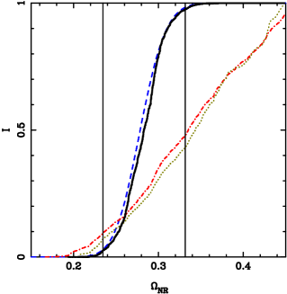
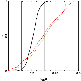
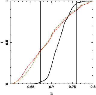
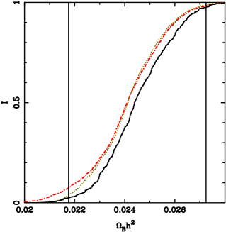
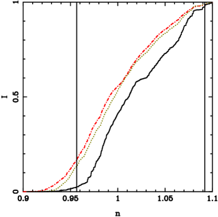
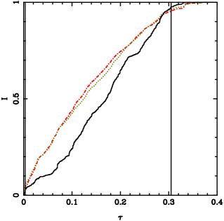
Figure 2: This Figure shows plots of $I$ (see eqn.9) for various parameters for the $\Lambda$CDM model. Red/dot-dashed curves show constraints from the WMAP observations of temperature anisotropies, dark-green/dotted curve shows constraints from WMAP observations and abundance of rich clusters, black/solid curve shows constraints from a combined analysis of WMAP observations, cluster abundance and high redshift supernovae. The blue/dashed curve shows the constraints from SN observations alone, this has been plotted only for the relevant parameters. Vertical lines mark the $95\%$ confidence limit for each parameter.

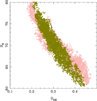
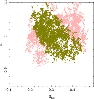
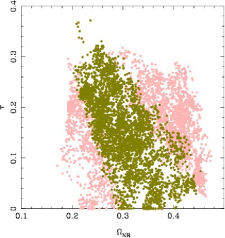
Figure 3: This Figure shows points in the Markov chain for $\Lambda$CDM models that are allowed by WMAP observations of temperature anisotropies in the CMB within $95\%$ confidence limit in the full parameter space (pink points). Models that are also allowed within a $99\%$ confidence limit by abundance of rich clusters of galaxies are shown as dark green points. The points are shown in a few projections to illustrate the fact that the requirement of cluster abundance rejects many models allowed by CMB observations. While for some projections it is clear that the region in parameter space allowed by cluster abundance is distinctly smaller than that allowed by CMB observations, in other projections these seem to have an almost complete overlap. This plot also highlights degeneracies in the parameter space.

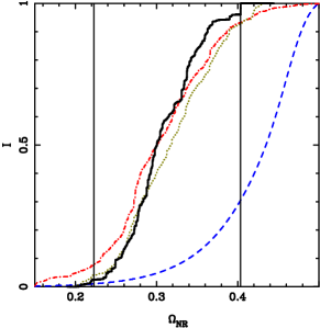
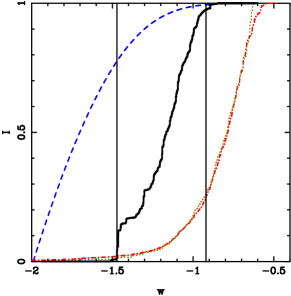
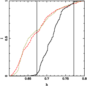
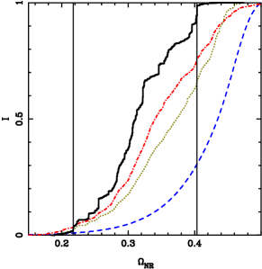
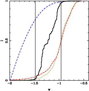
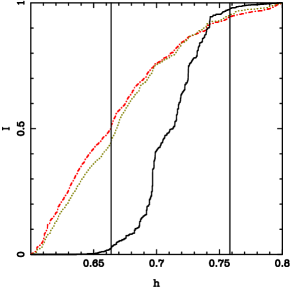
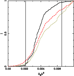
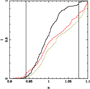
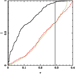
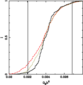
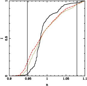
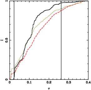
Figure 4: This figure shows $I$ for $\Omega_{NR}$, $w$ and $h$ for cosmological models with a constant equation of state parameter $w$. Panels in the first and third row are for models without perturbations in the dark energy component, whereas panels in second and fourth row are for models with perturbations in dark energy. Each panel shows $I$ derived from observations of high redshift supernovae, WMAP observations, WMAP observations combined with the constraints from abundance of rich clusters, and all three observations in combination (with the same color coding as in Fig. 2). We have marked $95\%$ confidence limits derived from using all the observations in concert as two vertical lines. The relevant parameters are written in the x-axis labels of the figures.

IV.2 Results in Detail

In this section we outline the detailed results of our analysis. We marginalize the results in the multi-dimensional parameter space to derive likelihood function for each parameter of interest. The likelihood function is sensitive to the bin-size used for the given parameter and tends to be somewhat noisy. It is customary to smooth the likelihood function with a Gaussian filter in order to remove noise but the results are sensitive to the width of the filter used. Therefore we choose to plot the cumulative likelihood as this is insensitive to binning and smoothing is not required. We define the cumulative likelihood as follows:

$$I(x)=\frac{\int\limits_{x_{min}}^{x}~{}\mathcal{L}(y)~{}dy}{\int\limits_{x_{min}}^{x_{max}}~{}\mathcal{L}(y)~{}dy}$$ (9)

where $x$ is the parameter we are interested in and it has a range $x_{min}\leq x\leq x_{max}$, $\mathcal{L}(x)$ is the likelihood obtained by marginalizing over other parameters. The central value for the given variable is thus $x_{c}$, with $I(x_{c})=0.5$. This can be, and in general it is different from the value of the parameter for maximum likelihood. $I(x)$ is like the cumulative probability function for the parameter $x$. Parameter values for which $I(x)=0.025$ and $I(x)=0.975$ define the range allowed at $95\%$ confidence limit, i.e. the probability that the variable lies within this range is $0.95$. We mark this limit by two vertical lines in all the likelihood plots.

IV.3 The $\Lambda$CDM model

Fig. 2 shows marginalized cumulative likelihood $I(x)$ for the $\Lambda$CDM model, different frames correspond to the different parameters we have considered here. Curves are shown for $\Omega_{NR}$, the shape parameter $\Gamma=\Omega_{NR}~{}h$, Hubble parameter $h=H_{0}/100~{}kms^{-1}Mpc^{-1}$, $\Omega_{b}~{}h^{2}$, spectral index $n$ and optical depth to the redshift of reionisation $\tau$. Red/dot-dashed curves show constraints from WMAP observations of CMB temperature anisotropies, dark-green/dotted curve shows constraints from WMAP observations and abundance of rich clusters, black/solid curve shows constraints from a combined analysis of WMAP observations, cluster abundance and high redshift supernovae. The blue/dashed curve shows the constraints from SN observations alone, this has been plotted only for $\Omega_{NR}$ as SN data does not constrain other parameters directly. Combined analysis for other parameters does have an input from supernova observations as many models allowed by WMAP and cluster abundance observations are ruled out by SN observations. Vertical lines mark the $95\%$ confidence limit when all the observations are used together. CMB observations allow considerable range for each of these parameters whereas observations of high redshift supernovae provide tight constraints. The reason why SN observations provide a tight constraint is clear from the discussion in the previous section, namely, SN observations favor models with $\Omega_{tot}\geq 1$. Within the context of models with $\Omega_{tot}=1$, SN observations favor models with $w\ll-1$. The $\Lambda$CDM model is only marginally allowed by SN observations within both the sets; flat $\Lambda$CDM models are allowed with $\mathcal{P}=0.12$ 2005A&A…429..807C and within flat models the $\Lambda$CDM model is allowed with $\mathcal{P}=0.06$.

The allowed range for all the parameters within $68\%$ confidence limit is given in Table 3 and range allowed in $95\%$ confidence limit is given in Table 4. Table 3 clearly illustrates the discrepancy between SN observations and WMAP observations. The values are comparable with those obtained in other analyses wmap_params ; 2004PhRvD..69j3501T . The range of values for the shape parameter $\Gamma=\Omega_{NR}h$ favored by these observations is consistent with values obtained from galaxy surveys 2004PhRvD..69j3501T ; sdss ; 2005astro.ph..1174C . The allowed range of values for $h$ are in agreement with direct determination 2001ApJ…553…47F .

Constraints from abundance of rich clusters do not make a significant impact on the likelihood function of individual parameters even though these constraints reject a significant fraction of models allowed by WMAP observations. To illustrate this, we have plotted points in the Markov chain for $\Lambda$CDM models that are allowed by WMAP observations in a few projections in the parameter space (Fig. 3). Also shown in the same plots are points allowed by abundance of rich clusters of galaxies. This clearly shows that the region in parameter space allowed by cluster abundance is distinctly smaller than that allowed by CMB observations. Well known degeneracies between parameters are also highlighted by this figure, e.g., there is a clear degeneracy between $\Omega_{NR}$ and $h$. An important point to note is that if the preferred range for $\sigma_{8}$ were to be towards larger values than taken here cluster4 ; 2003ApJ…591..599S then the cluster abundance constraint will favor models with larger $\Omega_{NR}$. There is also a related shift towards $w<-1$.

IV.4 Models with a constant $w$

We now consider models with a constant equation of state parameter $w$. Introduction of this additional parameter changes the relative effectiveness of different observations in constraining cosmological parameters. Observations of high redshift supernovae of type Ia constrain the key cosmological parameters much more strongly than CMB observations for $\Lambda$CDM models. This is no longer the case once we introduce $w$ as a parameter. The main reason for this is the degeneracy between $w$ and $\Omega_{NR}$.

In models with $w\neq 1$, it is necessary to take perturbations in the dark energy component into account 2004PhRvD..69h3503B ; perturb3 ; perturb4 . Here, we study models with and without perturbations in dark energy in order to illustrate the role played by these perturbations and to study how strongly these influence determination of cosmological parameters. Fig. 4 shows the likelihood $I$ for parameters $\Omega_{NR}$, $w$, $h$, $\Omega_{b}~{}h^{2}$, $n$ and $\tau$ in models with and without perturbations in the dark energy component. Models with a larger $\Omega_{NR}$ and smaller $w$ are better fits to SN observations, whereas CMB observations prefer models with smaller $\Omega_{NR}$ and a larger equation of state parameter $w$. The combination of these observations and abundance of rich clusters constrains both the parameters to a fairly narrow range, much narrower than is allowed by SN observations alone. Models with $w>-1$ fare badly with CMB observations when perturbations in the dark energy component are taken into account. For models with a constant $w$, observations allow higher values of $\Omega_{b}~{}h^{2}$ than for $\Lambda$CDM models. The allowed range in $\tau$ is smaller then the case with no dark energy perturbations whereas the ranges for $n$ are similar in both.

We find that the range of $w$ allowed at the $95\%$ confidence limit is smaller when perturbations in dark energy are allowed. For other parameters, the allowed range is similar. In other words, if we ignore perturbations in dark energy we can still make a reasonable estimate of the range of parameters allowed by observations. This fact is of immense use when we work with models that have a varying equation of state parameter $w$. In order to take full effects of dark energy perturbations in these models it is essential to know full details of the model 2004PhRvD..69h3503B ; perturb3 . We cannot include the effect of non-adiabatic perturbations in a model independent study of dark energy models with a varying $w$. Given the fact that ignoring perturbations in dark energy does not lead to an incorrect estimate of the range of parameters (except for $w$) that is allowed, we can safely proceed with our analysis without taking perturbations in dark energy into account. As regards the equation of state parameter $w$, ignoring perturbations tends to allow $w>-1$ models with a larger probability and we should keep this in mind while interpreting results.

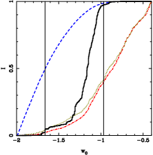
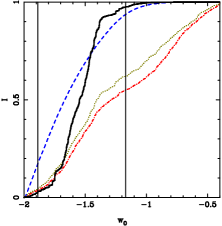
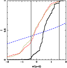
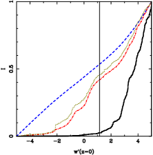
Figure 5: This figure shows $I$ for parameters that describe the variation of the equation of state parameter: $w_{0}$ and $w^{\prime}(z=0)$. Left panels are for $p=1$ and the right ones are for $p=2$. Color coding used is same as in figure 2.

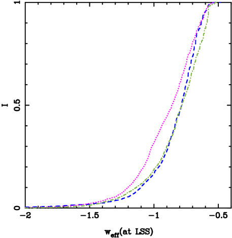
Figure 6: This figure shows $I$ for $w_{eff}$ at the redshift of surface of last scattering for the models with constant $w$ (blue/dashed curve), variable $w$ with $p=1$ (green/dot-dashed curve) and with $p=2$ (purple/dotted curve). Perturbations in dark energy are not taken into account in these models. See text for a more detailed description of this figure.

IV.5 Models with varying $w(z)$

We now proceed to the case of varying $w$, we use two parameterizations given in 2005MNRAS.356L..11J . The first of these, corresponding to $p=1$, is a Taylor series expansion for $w$ in scale factor and this is a very commonly used parameterization. The variation of the equation of state parameter is monotonic in this case and rapid increase of $w$ at low redshifts cannot be allowed as it will lead to $w\geq-1/3$ at high redshifts. The parameterization with $p=2$ avoids this problem to some extent as the value of $w$ at very high redshifts is the same as the present value, but there can be a large deviation from this at low redshifts with the deviation peaking at $z=1$. Rapid variation at low red-shifts has been reported 2004MNRAS.354..275A on the basis of SN observations nova_data1 ; nova_data3 , and even though these conclusions have been contested dynamic_de6 it is useful to check if the larger set of observations support a rapid variation of $w$ at low redshifts.

We have already seen in the discussion of fiducial models, supernova observations do not distinguish between models with a constant $w$ and models with a variable equation of state parameter. Also, WMAP observations do not differentiate between the three classes of models being studied here in a statistically significant manner.

Fig. 5 shows the allowed ranges of parameters $w_{0}$ and $w^{\prime}(z=0)$ for $p=1$ (left panels) and $p=2$ (right panels). In both the parameterizations, the preferred values for $w_{0}$ with supernova observations are for phantom models ($w_{0}\leq-1$) and a tendency for a larger $w$ at intermediate redshift, i.e., $w^{\prime}_{0}\geq 0$ though supernova observations do not provide a clear constraint on this parameter. This is perhaps related to the fact that there is a strong degeneracy in $\Omega_{NR}$ and $w_{0}$. CMB observations and abundance of rich clusters of galaxies allow models around the $\Lambda$CDM model, which is fairly close to the centre of the allowed region. A combination of these three observations rejects models with $w_{0}\ll-1$ due to CMB constraints and $w_{0}>-1$ due to SN constraints. Even though all the observations allow $w^{\prime}_{0}=0$, the combination of these observations does not favor such models. This implies that the overlap of allowed regions for the three observations is stronger for models with $w^{\prime}_{0}\neq 0$, it is clear from table 3 that there is no overlap between SN and WMAP at $68\%$ confidence limit for constant $w$. The $\Lambda$CDM model, i.e., $w_{0}=-1$ and $w^{\prime}_{0}=0$ is a marginally allowed model for both the parameterizations.

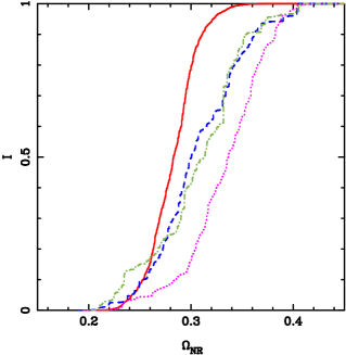
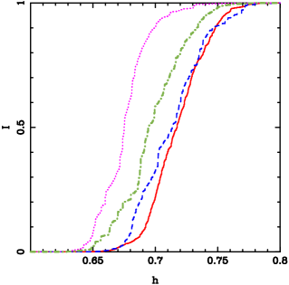
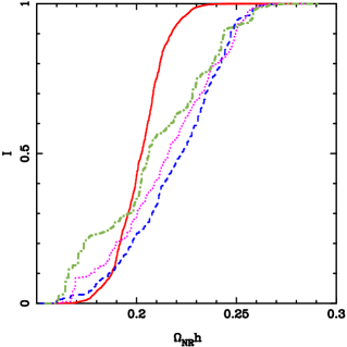
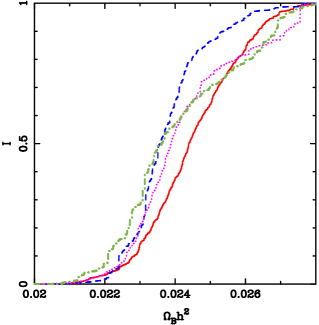
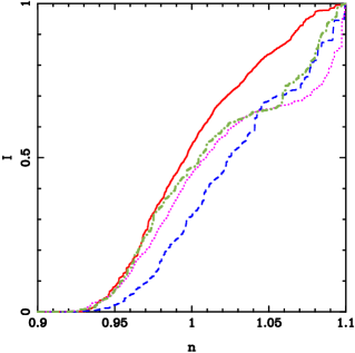
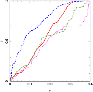
Figure 7: Panels for $\Omega_{NR}$, $h$, $\Gamma=\Omega_{NR}~{}h$, $\Omega_{b}~{}h^{2}$, $n$ and $\tau$. Red/solid curve is for $\Lambda$CDM, blue/dashed curve for models with constant $w$, green/dot-dashed for $p=1$ and purple/dotted curve for $p=2$.

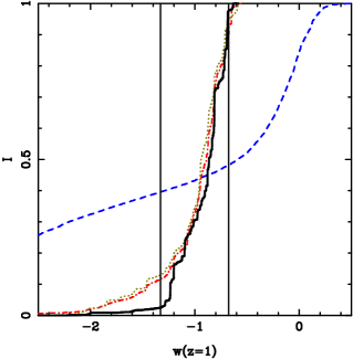
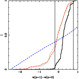
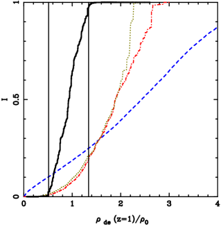
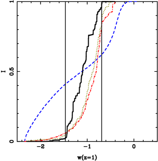
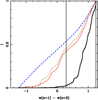
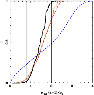
Figure 8: The top and bottom panels in the figure correspond to parameterizations with $p=1$ and $p=2$ respectively. The figures on the left show likelihood for the equation of state parameter $w$ at redshift $z=1$ for models which have equation of state lying within the range $-1.1<w_{0}<-0.9$. In the middle panel we plot the likelihood for variation in the equation of state parameter from the present value at redshift $z=1$. The third panel shows the allowed range of change in the dark energy density upto $z=1$. Color coding is same as in Fig. 2

To understand the nature of constraint from CMB observations 2003MNRAS.343..533D , we computed the likelihood of $w_{eff}$ (as defined in eqn.(8)) for models by comparing these with WMAP data. This is then compared with the likelihood for $w$ in models with a constant equation of state parameter. We have plotted this in Fig. 6 for $p=1$ as well as $p=2$, along with the curve for constant $w$ (with no perturbations in dark energy). All the three curves show very similar behavior and the $95\%$ confidence limit is identical for all three ($-1.5\leq w_{eff}\leq-0.6$). This also shows that the CMB observations primarily provide a constraint for $w_{eff}$. Given that adding perturbations reduces the likelihood for models with $w>-1$, it is likely that detailed analysis of a model with perturbations in dark energy taken into account will limit the range for $w_{eff}$ in this region.

Lastly, we study the effect of varying dark energy on other parameters. The specific question we wish to address is, how the allowed ranges for these parameters change if we allow variation of dark energy. Fig. 7 shows likelihood for the parameters studied here. We have plotted the likelihood using all three observations for the $\Lambda$CDM models, constant $w$ models as well as for $p=1$ and $p=2$. For most parameters, the effect of $w\neq-1$ and varying dark energy is to increase the range of allowed values. This increase in the allowed range is sometimes accompanied by a shift, e.g. for $h$ where varying dark energy models fit observations better with smaller values as compared to the $\Lambda$CDM model as well as models with constant $w$. This shift is primarily due to models with $w>-1$ and this point has been noted in other analyses as well wmap_params . If this is the case then including perturbations in dark energy may well remove this shift.

Similarly, larger values of spectral index $n$ and optical depth to the epoch of reionisation $\tau$ fit observations better. As these parameters can be constrained using other observations, we may be able to restrict models with varying $w$ by constraining the values of these parameters. For example, polarization anisotropies in the CMB can be used to constrain $\tau$ cmbrev1 ; 2003ApJ…583…24K . We find that the presently available information from WMAP about polarization anisotropies does not lead to a significantly improved constraint on the parameter $\tau$.

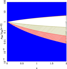
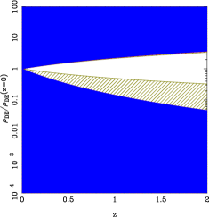
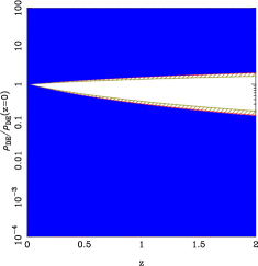
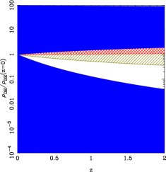
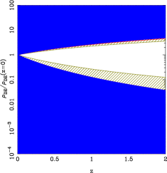
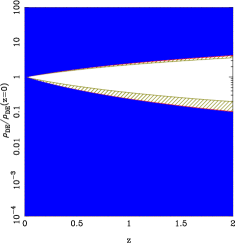
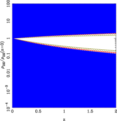
Figure 9: In this figure we plot evolution of dark energy density as a function of redshift. The top panel is for models without dark energy perturbations and the lower panel is with dark energy perturbations included. The left plot in both the rows shows the variation in energy density allowed by Supernova observations. The green/hatched region is excluded at $68\%$ confidence level, red/cross-hatched at $95\%$ confidence level and blue/solid at $99\%$ confidence level. The white region is the allowed region in variation at $68\%$ significance level. The plot which is second from left (in both the cases) displays the allowed range by WMAP data alone, color scheme being the same as in left figure. The next figure shows allowed range by WMAP and cluster abundance observations. The last column shows contribution from combined analysis of the three observations.

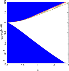
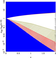
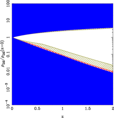
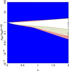
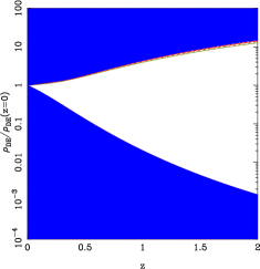
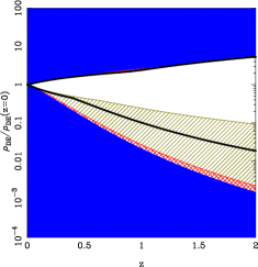
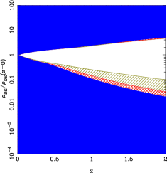
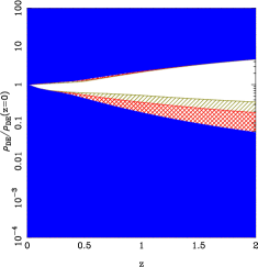
Figure 10: Same as figure 9 but for varying dark energy models. The top panel is for $p=1$ and the lower panel is for $p=2$. Starting from left, the figures show allowed dark energy density variation from SN observations, WMAP observations, WMAP observations combined with cluster abundance requirements and by combined analysis. The region enclosed by black solid lines (lower panel, second frame from left) is obtained from the derived constraints on $w_{eff}$, see text for details.

IV.6 Evolution of dark energy

We now summarize our results for the allowed variation of dark energy, once all three observational constraints have been taken into account. In the left panel of Fig. 8, we have plotted the cumulative likelihood for the equation of state parameter $w$ at redshift $z=1$. Here we have used models which lie within the range $-1.1<w_{0}<-0.9$. The upper and lower panels correspond to parameterizations with $p=1$ and $p=2$ respectively. The allowed range of variation in the equation of state by supernova observations is much larger than that allowed by WMAP results. This, again, is a reflection of the strong preference of supernova observations for $w\ll-1$ and of the large parameter space allowed by SN data. (Our result that SN data prefers $w\ll-1$ with large variation is consistent with previous published analysis e.g., in 2004ApJ…617L…1B .) The range of values in both the parameterizations are similar for this subset of models. In the middle panel we have shown the likelihood for variation in the equation of state parameter from the present to its value at redshift $z=1$. The allowed ranges of variation in dark energy equations of state are different for these two parameterizations. In fact, the constant dark energy equation of state is ruled out at $95\%$ confidence level for $p=2$ (that is, the probability of occurrence is less than $0.05$) when all the constraints are taken into account even though each observational constraint allows such models individually. Clearly, the models with constant $w$ allowed by each of these observations are ruled out by other observations. The $\Lambda$CDM model is allowed for $p=2$ at $77\%$ C.L. (with probability of $23\%$) by SN observations and by $0.9\%$ C.L. ($\mathcal{P}=0.991$) by WMAP observations.

In the right panel, we have shown the ratio of dark energy density at $z=1$ and the present value. The variation allowed by SN observations is very large, whereas WMAP limits the variation to within a factor $2.5$ at $95\%$ confidence limits. This drives the joint analysis to restrict variation even further. That WMAP observations provide a much tighter constraint on the equation of state as compared to SN observations was earlier shown in 2005MNRAS.356L..11J .

In Fig. 9 we show the allowed range of variation of dark energy as function of redshift for $w=constant$ models, with and without perturbations at $68\%$, $95\%$ and $99\%$ confidence levels. The figure shows the disparity in allowed range by SN observations and WMAP observations at $68\%$ confidence level. Allowing perturbations in dark energy gives a similar range as compared to the case where dark energy perturbations are absent. In Fig. 10 we plot this range for varying dark energy models, top panel for models with $p=1$ and lower panel for $p=2$. As mentioned earlier (see also 2005MNRAS.356L..11J ), SN observations allow a much wider range in change of dark energy density with redshift. The variation allowed by WMAP is smaller in all cases except constant $w$. The combination of the three constraints allows very little variation, with maximum allowed variation in dark energy density being by a factor $5$ up to $z=2$ at $68\%$ confidence limit. The allowed variation in dark energy density is similar in both the cases, indicating that the constraints on this quantity are parameterization independent to a large extent.

Finally, we would like to make some comments regarding the fact that WMAP constrains the evolution of dark energy more effectively than SN. This arises essentially from the constraint on the angular diameter distance to the last scattering surface, or — equivalently — the effective equation of state parameter $w_{eff}$. (The Integrated Sachs-Wolfe effect and the contribution of other parameters turns out to be less important.) To illustrate this point, we have compared the constraints on dark energy density for $p=2$ with those implied by constraints on $w_{eff}$. The second figure in the lower panel in Fig. 10 shows the allowed range in evolution of dark energy density allowed by WMAP data alone for $p=2$. We have also plotted the allowed range for dark energy density as a function of redshift if $-1.6\leq w_{eff}\leq-0.6$, by thick black lines. This is derived by using all $w_{0}$ and $w^{\prime}_{0}$ that lead to $w_{eff}$ in the range given above, and computing the highest and lowest dark energy density amongst this set of models at each redshift. We allow $w_{0}$ and $w^{\prime}_{0}$ to vary in the range specified in the priors. The region allowed by the range in $w_{eff}$ and that directly obtained from all allowed models is similar, with the latter allowing larger variation for phantom models. This reiterates our claim that the main constraint from WMAP data on dark energy parameters is on the value of $w_{eff}$ at the last scattering surface. We believe that the larger range allowed at $95\%$ confidence limit is due mainly to the ISW effect.

Table 3: This table lists the range of relevant parameters allowed within 68% confidence limit from SN, WMAP, WMAP + cluster abundance (CA) requirements and after combining all observations.

Parameter	$\Lambda$CDM	w=const.	w=const.	p=1	p=2
			with perturbations
	$0.256$—$0.3$	$0.37$—$0.47$	$0.37$—$0.47$	$0.19$—$0.47$	$0.18$—$0.47$	SN
	$0.26$—$0.42$	$0.25$—$0.37$	$0.28$—$0.42$	$0.22$—$0.39$	$0.21$—$0.37$	WMAP
$\Omega_{NR}$	$0.265$—$0.424$	$0.26$—$0.38$	$0.29$—$0.43$	$0.24$—$0.42$	$0.24$—$0.4$	WMAP+CA
	$0.26$—$0.3$	$0.27$—$0.35$	$0.26$—$0.38$	$0.26$—$0.35$	$0.3$—$0.37$	SN+WMAP+CA
		$-1.9$ — $-1.39$	$-1.9$ — $-1.39$	$-1.89$ — $-1.31$	$-1.9$ — $-1.33$	SN
		$-1.0$ — $-0.67$	$-1.2$ — $-0.77$	$-1.19$ — $-0.56$	$-1.67$ — $-0.7$	WMAP
$w_{0}$		$-1.02$ — $-0.67$	$-1.13$ — $-0.78$	$-1.28$ — $-0.56$	$-1.71$ — $-0.75$	WMAP+CA
		$-1.41$ — $-1.02$	$-1.37$ — $-1.04$	$-1.3$ — $-1.05$	$-1.69$ — $-1.4$	SN+WMAP+CA
				$-3.2$ — $3.46$	$-3.3$ — $3.99$	SN
				$-0.94$ — $0.67$	$-0.74$ — $4.15$	WMAP
$w^{\prime}(z=0)$				$-1.0$ — $0.75$	$-1.03$ — $3.94$	WMAP+CA
				$0.21$ — $1.06$	$2.74$ — $4.58$	SN+WMAP+CA

Table 4: This table lists the range of parameters allowed within 95% confidence limit from SN, WMAP, WMAP + cluster abundance (CA) requirements and after combining all observations.

Parameter	$\Lambda$CDM	w=const.	w=const.	p=1	p=2
			with perturbations
	$0.23$ — $0.33$	$0.27$ — $0.49$	$0.27$ — $0.495$	$0.11$ — $0.49$	$0.11$ — $0.49$	SN
	$0.20$ — $0.45$	$0.16$ — $0.43$	$0.20$ — $0.47$	$0.17$ — $0.45$	$0.18$ — $0.44$	WMAP
$\Omega_{NR}$	$0.22$ — $0.44$	$0.21$ — $0.42$	$0.22$ — $0.46$	$0.21$ — $0.46$	$0.2$ — $0.44$	WMAP+CA
	$0.23$ — $0.33$	$0.22$ — $0.4$	$0.22$ — $0.4$	$0.21$ — $0.403$	$0.23$ — $0.39$	SN+WMAP+CA
		$-1.97$ — $-1.1$	$-1.97$ — $-1.1$	$-1.97$ — $-1.03$	$-1.97$ — $-1.05$	SN
		$-1.39$ — $-0.58$	$-1.6$ — $-0.63$	$-1.64$ — $-0.42$	$-1.93$ — $-0.43$	WMAP
$w_{0}$		$-1.34$ — $-0.63$	$-1.4$ — $-0.66$	$-1.73$ — $-0.42$	$-1.95$ — $-0.47$	WMAP+CA
		$-1.47$ — $-0.91$	$-1.48$ — $-0.96$	$-1.66$ — $-0.97$	$-1.89$ — $-1.17$	SN+WMAP+CA
				$-4.72$ — $4.6$	$-4.73$ — $4.85$	SN
				$-3.09$ — $1.32$	$-2.5$ — $4.87$	WMAP
$w^{\prime}(z=0)$				$-3$ — $1.35$	$-2.7$ — $4.8$	WMAP+CA
				$-0.38$ — $1.54$	$1.15$ — $4.99$	SN+WMAP+CA
$w_{eff}(atLSS)$		$-1.4$ — $-0.5$		$-1.48$ — $-0.59$	$-1.41$ — $-0.58$
	$0.02$ — $0.027$	$0.021$ — $0.028$	$0.02$ — $0.027$	$0.02$ — $0.027$	$0.02$ — $0.027$	WMAP
$\Omega_{b}~{}h^{2}$	$0.021$ — $0.027$	$0.022$ — $0.028$	$0.022$ — $0.027$	$0.021$ — $0.027$	$0.022$ — $0.028$	WMAP+CA
	$0.022$ — $0.027$	$0.022$ — $0.027$	$0.022$ — $0.027$	$0.021$ — $0.027$	$0.022$ — $0.028$	SN+WMAP+CA
	$0.61$ — $0.79$	$0.61$ — $0.78$	$0.6$ — $0.79$	$0.6$ — $0.78$	$0.61$ — $0.78$	WMAP
$h$	$0.61$ – $0.78$	$0.61$ — $0.77$	$0.61$ — $0.78$	$0.61$ — $0.7$8	$0.6$ — $0.78$	WMAP+CA
	$0.67$ — $0.76$	$0.67$ — $0.77$	$0.66$ — $0.76$	$0.65$ — $0.75$	$0.64$ — $0.72$	SN+WMAP+CA
	$0.002$ — $0.33$	$0.011$ — $0.39$	$0.007$ — $0.35$	$0.13$ — $0.4$	$0.016$ — $0.39$	WMAP
$\tau$	$0.001$ — $0.32$	$0.028$ — $0.36$	$0.006$ — $0.35$	$0.01$ — $0.37$	$0.015$ — $0.387$	WMAP+CA
	$0.003$ — $0.3$	$0.002$ — $0.29$	$0.022$ — $0.26$	$0.006$ — $0.38$	$0.01$ — $0.39$	SN+WMAP+CA
	$0.93$ — $1.08$	$0.93$ — $1.1$	$0.93$ — $1.09$	$0.93$ — $1.1$	$0.93$ — $1.09$	WMAP
$n$	$0.94$ — $1.09$	$0.94$ — $1.1$	$0.94$ — $1.09$	$0.94$ — $1.09$	$0.94$ — $1.09$	WMAP+CA
	$0.96$ — $1.09$	$0.94$ — $1.08$	$0.95$ — $1.08$	$0.94$ — $1.09$	0$.93$ — $1.09$	SN+WMAP+CA

V Conclusions

In this paper we presented a detailed analysis of constraints on cosmological parameters from different observations. In particular we focussed on constraints on dark energy equation of state, its present value and the allowed range of variation in it.

It is demonstrated that the allowed range for the equation of state parameter $w$ is smaller if dark energy is allowed to cluster. Including perturbations mainly affects models with $w>-1$.

We find that WMAP observations do not distinguish between the $\Lambda$CDM model, models with a constant equations of state parameter $w$ and models with a variable $w$, the change in $\chi^{2}_{W}$ for best fit models is less than $3$ even as the number of parameters is increased by three. WMAP allows only a modest variation in energy density of dark energy, with maximum variation being less than a factor of three in $99\%$ confidence limit up to $z=1$. We infer that the main constraint from WMAP observations is for the derived quantity $w_{eff}$, essentially representing the distance to the last scattering surface.

SN observations favour models with $w<-1$ and $\Omega_{nr}>0.4$. A corollory is that if we restrict to models with $w\geq-1$ then the $\Lambda$CDM model is the most favoured model. Without this restriction the $\Lambda$CDM model is allowed only marginally by the combination of observations used here, this is driven mainly by SN observations.

Allowing variation in dark energy has an impact on other cosmological parameters as the allowed range for many of these parameters becomes larger. Conversely, better measurements of these parameters will allow us to constrain models of dark energy.

We find significant tension between different observations. Our key conclusions in this regard may be summarised as follows:

• SN observations favor models with large $\Omega_{NR}$ and $w\ll-1$. Indeed, the best fit model is at the edge of our priors.

• Enlarging priors to $0.1\leq\Omega_{NR}\leq 0.6$, $-0.3\geq w\geq-3.0$ does not lead to a better fit model for SN observations, indicating that our default priors are sufficiently wide for joint estimation of parameters. This is because $w\ll-1$ is rejected by WMAP observations.

• WMAP observations favor models with $w\sim-1$ with a marginal preference for $w>-1$. Including perturbations in dark energy removes this marginal preference as well.

• For constant $w$ models and models with variable $w$, the best fit model of each observation is ruled out by the other observations at a high significance level. As an example, the model that best fits the WMAP observations is completely ruled out by SN observations ($\Delta\chi_{S}^{2}=53$). The problem is slightly less serious if perturbations in dark energy are taken into account ($\Delta\chi_{S}^{2}=12.5$).

• There is overlap of allowed regions at $95\%$ (or better) by these observations, though there is little overlap of allowed regions at $68\%$ confidence limit (see table 3). It can, of course, be argued that situation is not alarming given that there is an overlap of allowed regions in parameter space at $95\%$. But we find this offset noteworthy.

• Using larger values for $\sigma_{8}$, as indicated by some recent analyses cluster4 ; 2003ApJ…591..599S favors models with a slightly larger $\Omega_{NR}$ and slightly lower $w_{eff}$.

• Given that the preference of individual observations for different types of models is not understood, and the fact that the best fit model of one is ruled out by the other, it is necessary to use a combination of observations for reliable constraints on models of dark energy. Use of either one of the observations is likely to mislead.

• Our conclusions are not sensitive to priors used for parameters other than $\Omega_{NR}$. Limiting priors for matter density to $0.1\leq\Omega_{NR}\leq 0.3$ enhances the overlap between SN and WMAP observations and removes the tension between SN and WMAP observations for constant $w$ models.

• If we repeat the analysis of models with variable $w$ with this restricted priors then we find that SN observations strongly favor a variable $w$ as compared to constant $w$. There is no significant tension between SN and WMAP models in this class of models even for the wider priors, but this is mainly due to a larger number of parameters.

• Using only the Gold data set for supernovae instead of the Gold $+$ Silver used here reduces the tension between the WMAP and supernova observations by a marginal amount.

Given the points noted here regarding tension between different observations, it is important that some effort is made to look for systematic effects in observations as well as in analysis of observations. We have tested our analysis for systematic effects by varying priors and our findings appear to be independent of the chosen priors, the only instance of change in results is mentioned above. Since the SN data set which is used by most people (including in this work) arises from different sources, one needs to be careful regarding hidden systematics (see e.g., the discussion in saul ). When larger, homogeneous SN datasets are available in future (like for example, from SNLS), it is likely that the tension between the SN observations and WMAP results disappear. If it does not, and the agreement continues to exist only at 3-sigma level, there is some cause for concern.

References

- (1) J. P. Ostriker and P. J. Steinhardt, Nature (London) 377, 600 (1995). S. D. M. White, J. F. Navarro, A. E. Evrard, and C. S. Frenk, Nature (London) 366, 429 (1993). J. S. Bagla, T. Padmanabhan, and J. V. Narlikar, Comments on Astrophysics 18, 275 (1996), eprint arXiv:astro-ph/9511102 ; G. Efstathiou, W. J. Sutherland, and S. J. Maddox, Nature (London) 348, 705 (1990).
- (2) J. L. Tonry, B. P. Schmidt, B. Barris, P. Candia, P. Challis, A. Clocchiatti, A. L. Coil, A. V. Filippenko, P. Garnavich, C. Hogan, et al., Astrophys. J. 594, 1 (2003); B. J. Barris, J. L. Tonry, S. Blondin, P. Challis, R. Chornock, A. Clocchiatti, A. V. Filippenko, P. Garnavich, S. T. Holland, S. Jha, et al., Astrophys. J. 602, 571 (2004).
- (3) A. G. Riess, L. Strolger, J. Tonry, S. Casertano, H. C. Ferguson, B. Mobasher, P. Challis, A. V. Filippenko, S. Jha, W. Li, et al., Astrophys. J. 607, 665 (2004).
- (4) A. Melchiorri, P. A. R. Ade, P. de Bernardis, J. J. Bock, J. Borrill, A. Boscaleri, B. P. Crill, G. De Troia, P. Farese, P. G. Ferreira, et al., Astrophys. J. Lett. 536, L63 (2000).
- (5) D. N. Spergel, L. Verde, H. V. Peiris, E. Komatsu, M. R. Nolta, C. L. Bennett, M. Halpern, G. Hinshaw, N. Jarosik, A. Kogut, et al., Astrophys. J. Suppl. 148, 175 (2003).
- (6) E. Hawkins, S. Maddox, S. Cole, O. Lahav, D. S. Madgwick, P. Norberg, J. A. Peacock, I. K. Baldry, C. M. Baugh, J. Bland-Hawthorn, et al., Mon. Not. Roy. Astron. Soc. 346, 78 (2003).
- (7) A. C. Pope, T. Matsubara, A. S. Szalay, M. R. Blanton, D. J. Eisenstein, J. Gray, B. Jain, N. A. Bahcall, J. Brinkmann, T. Budavari, et al., Astrophys. J. 607, 655 (2004).
- (8) S. L. Bridle, O. Lahav, J. P. Ostriker, and P. J. Steinhardt, Science 299, 1532 (2003).
- (9) M. Tegmark, M. A. Strauss, M. R. Blanton, K. Abazajian, S. Dodelson, H. Sandvik, X. Wang, D. H. Weinberg, I. Zehavi, N. A. Bahcall, et al., Phys. Rev. D 69, 103501 (2004).
- (10) T. Padmanabhan, (2005), eprint arXiv:gr-qc/0503107.
- (11) S. Weinberg, Rev. Mod. Phys. 61, 1 (1989).
- (12) T. Padmanabhan, Phys. Rept. 380, 235 (2003),eprint arXiv:hep-th/0212290; P. J. Peebles and B. Ratra, Rev. Mod. Phys. 75, 559 (2003); V. Sahni and A. Starobinsky, Int.Jour.Mod.Phys.D 9, 373 (2000); J. Ellis, Royal Society of London Philosophical Transactions Series A 361, 2607 (2003); T. Padmanabhan, (2004a), eprint arXiv:astro-ph/0411044.
- (13) P. J. Steinhardt, Royal Society of London Philosophical Transactions Series A 361, 2497 (2003); A. D. Macorra and G. Piccinelli, Phys. Rev. D 61, 123503 (2000); L. A. Ureña-López and T. Matos, Phys. Rev. D 62, 081302 (2000); P. F. González-Díaz, Phys. Rev. D 62, 023513 (2000a); R. de Ritis and A. A. Marino, Phys. Rev. D 64, 083509 (2001); S. Sen and T. R. Seshadri, Int.Jour.Mod.Phys.D 12, 445 (2003); C. Rubano and P. Scudellaro, Gen. Rel. Grav. 34, 307 (2002), eprint astro-ph/0103335; S. A. Bludman and M. Roos, Phys. Rev. D 65, 043503 (2002).
- (14) C. Armendariz-Picon, V. Mukhanov, and P. J. Steinhardt, Phys. Rev. D 63, 103510 (2001); T. Chiba, Phys. Rev. D 66, 063514 (2002); M. Malquarti, E. J. Copeland, A. R. Liddle, and M. Trodden, Phys. Rev. D 67, 123503 (2003); L. P. Chimento and A. Feinstein, Mod. Phys. Letts. A 19, 761 (2004); R. J. Scherrer, Phys. Rev. Letts. 93, 011301 (2004).
- (15) T. Padmanabhan, Phys. Rev. D 66, 021301 (2002).
- (16) J. S. Bagla, H. K. Jassal, and T. Padmanabhan, Phys. Rev. D 67, 063504 (2003), eprint arXiv:astro-ph/0212198; H. K. Jassal, (2003a), eprint arXiv:astro-ph/0303406; J. M. Aguirregabiria and R. Lazkoz, Phys. Rev. D 69, 123502 (2004); A. Sen, (2003), eprint arXiv:hep-th/0312153; V. Gorini, A. Kamenshchik, U. Moschella, and V. Pasquier, Phys. Rev. D 69, 123512 (2004); G. W. Gibbons, Class. Quan. Grav. 20, 321 (2003a); C. Kim, H. B. Kim, and Y. Kim, Phys. Letts. B 552, 111 (2003); G. Shiu and I. Wasserman, Phys. Letts. B 541, 6 (2002); D. Choudhury, D. Ghoshal, D. P. Jatkar, and S. Panda, Phys. Letts. B 544, 231 (2002); A. Frolov, L. Kofman, and A. Starobinsky, Phys. Letts. B 545, 8 (2002); G. W. Gibbons, Phys. Letts. B 537, 1 (2002); A. Das, S. Gupta, T. Deep Saini, and S. Kar, (2005), eprint arXiv:astro-ph/0505509; I. Y. Aref’eva, (2004), eprint arXiv:astro-ph/0410443.
- (17) R. R. Caldwell, Phys. Letts. B 545, 23 (2002); J. Hao and X. Li, Phys. Rev. D 68, 043501 (2003a); G. W. Gibbons, (2003b), eprint arXiv:hep-th/0302199; V. K. Onemli and R. P. Woodard, Phys. Rev. D 70, 107301 (2004a); S. Nojiri and S. D. Odintsov, Phys. Letts. B 562, 147 (2003); S. M. Carroll, M. Hoffman, and M. Trodden, Phys. Rev. D 68, 023509 (2003); P. Singh, M. Sami, and N. Dadhich, Phys. Rev. D 68, 023522 (2003); P. H. Frampton, Mod. Phys. Letts. A 19, 801 (2004); J. Hao and X. Li, Phys. Rev. D 67, 107303 (2003b); P. González-Díaz, Phys. Rev. D 68, 021303 (2003a); M. P. Dabrowski, T. Stachowiak, and M. Szydłowski, Phys. Rev. D 68, 103519 (2003); J. M. Cline, S. Jeon, and G. D. Moore, Phys. Rev. D 70, 043543 (2004); W. Fang, H. Q. Lu, Z. G. Huang, and K. F. Zhang, ArXiv High Energy Physics - Theory e-prints (2004), eprint arXiv:hep-th/0409080; S. Nojiri and S. D. Odinstov, ArXiv High Energy Physics - Theory e-prints (2005), eprint arXiv:hep-th/0505215; S. Nesseris and L. Perivolaropoulos, Phys. Rev. D 70, 123529 (2004); S. Nojiri and S. D. Odinstov, Phys. Rev. D 70, 103522 (2004); E. Elizalde, S. Nojiri and S. D. Odinstov, Phys. Rev. D 70, 043539 (2004); S. Nojiri, S. D. Odinstov, and S. Tsujikawa, Phys. Rev. D 71, 063004 (2005).
- (18) K. Uzawa and J. Soda, Mod. Phys. Letts. A 16, 1089 (2001); H. K. Jassal, (2003b), eprint arXiv:hep-th/0312253; C. P. Burgess, Int.Jour.Mod.Phys.D 12, 1737 (2003); K. A. Milton, Grav. Cosmol. 9, 66 (2003), eprint hep-ph/0210170; P. F. González-Díaz, Phys. Letts. B 481, 353 (2000b).
- (19) R. Holman and S. Naidu, (2004), eprint arXiv:astro-ph/0408102.
- (20) T. Padmanabhan, (2004b), eprint arXiv:hep-th/0406060; I. Shapiro and J. Sola JHEP 006 (2002), eprint arXiv:hep-th/0012227; J. Sola and H. Stefancic, (2005), eprint arXiv:astro-ph/0505133.
- (21) T. Padmanabhan and T. R. Choudhury, Phys. Rev. D 66, 081301 (2002); V. F. Cardone, A. Troisi, and S. Capozziello, Phys. Rev. D 69, 083517 (2004); P. F. González-Díaz, Phys. Letts. B 562, 1 (2003b); M. A. M. C. Calik, (2005), eprint arXiv:gr-qc/0505035; S. Capozziello, S. Nojiri and S. D. Odintsov, (2005), eprint arXiv:hep-th/0507182.
- (22) V. K. Onemli and R. P. Woodard, Class. Quant. Grav. 19, 4607 (2002), T. Padmanabhan, Phys. Reports, 49, 406,2005 eprint arXiv:gr-qc/0311036; T. Padmanabhan, Class.Quant.Grav, 19, 5387,2002 eprint arXiv:gr-qc/0204019; A. A. Andrianov, F. Cannata, and A. Y. Kamenshchik, (2005), eprint arXiv:gr-qc/0505087; R. Lazkoz, S. Nesseris and L. Perivolaropoulos, (2005), eprint arXiv:astro-ph/0503230; M. Szydlowski, W. Godlowski and R. Wojtak, (2005), eprint arXiv:astro-ph/0503202.
- (23) H. K. Jassal, J. S. Bagla, and T. Padmanabhan, Mon. Not. Roy. Astron. Soc. Lett. 356, L11 (2005),eprint arXiv:astro-ph/0404378.
- (24) T. R. Choudhury and T. Padmanabhan, Astron. Astrophys. 429, 807 (2005) eprint arXiv:astro-ph/0311622.
- (25) U. Seljak, A. Makarov, P. McDonald, S. F. Anderson, N. A. Bahcall, J. Brinkmann, S. Burles, R. Cen, M. Doi, J. E. Gunn, et al., Phys. Rev. D 71, 103515 (2005).
- (26) Y. Wang, V. Kostov, K. Freese, J. A. Frieman, and P. Gondolo, (2004), eprint arXiv:astro-ph/0402080.
- (27) B. A. Bassett, P. S. Corasaniti, and M. Kunz, Astrophys. J. Lett. 617, L1 (2004).
- (28) S. Lee, (2005), eprint arXiv:astro-ph/0504650.
- (29) M. Li, Phys. Letts. B 603, 1 (2004).
- (30) S. Hannestad and E. Mörtsell, JCAP 9, 1 (2004).
- (31) M. Chevallier and D. Polarski, Int. J. Mod. Phys. D10, 213 (2001); E. V. Linder, Phys. Rev. Lett. , 90, 091301 (2003)
- (32) M. Hamuy, M. M. Phillips, N. B. Suntzeff, R. A. Schommer, J. Maza, A. R. Antezan, M. Wischnjewsky, G. Valladares, C. Muena, L. E. Gonzales, et al., Astrophys. J. 112, 2408 (1996); A. G. Riess, A. V. Filippenko, P. Challis, A. Clocchiatti, A. Diercks, P. M. Garnavich, R. L. Gilliland, C. J. Hogan, S. Jha, R. P. Kirshner, et al., Astron. J. 116, 1009 (1998); S. Perlmutter, G. Aldering, G. Goldhaber, R. A. Knop, P. Nugent, P. G. Castro, S. Deustua, S. Fabbro, A. Goobar, D. E. Groom, et al., Astrophys. J. 517, 565 (1999a); A. G. Riess, R. P. Kirshner, B. P. Schmidt, S. Jha, P. Challis, P. M. Garnavich, A. A. Esin, C. Carpenter, R. Grashius, R. E. Schild, et al., Astron. J. 117, 1009 (1999); A. G. Riess, P. E. Nugent, R. L. Gilliland, B. P. Schmidt, J. Tonry, M. Dickinson, R. I Thompson, T. Budavári, S. Casertano, A. S. Evans, et al., Astrophys. J. 560, 49 (2001a); R. A. Knop, G. Aldering, R. Amanullah, P. Astier, G. Blanc, M. S. Burns, A. Conley, S. E. Deustua, M. Doi, R. Ellis, et al., Astrophys. J. 598, 102 (2003); P. M. Garnavich, S. Jha, P. Challis, A. Clocchiatti, A. Diercks, A. V. Filippenko, R. L. Gilliland, C. J. Hogan, R. P. Kirshner, B. Leibundgut, et al., Astrophys. J. 509, 74 (1998).
- (33) T. Padmanabhan and T. R. Choudhury, Mon. Not. Roy. Astron. Soc. 344, 823 (2003) eprint arXiv:astro-ph/0212573.
- (34) U. Alam, V. Sahni, T. Deep Saini, and A. A. Starobinsky, Mon. Not. Roy. Astron. Soc. 344, 1057 (2003); U. Alam, V. Sahni, and A. A. Starobinsky, JCAP 6, 8 (2004).
- (35) Y. Wang and M. Tegmark, Phys. Rev. Letts. 92, 241302 (2004); Y. Wang, New Astronomy Review 49, 97 (2005).
- (36) D. Eisenstein and M. White, Phys. Rev. D 70, 103523 (2004).
- (37) D. J. Eisenstein, I. Zehavi, D. W. Hogg, R. Scoccimarro, M. R. Blanton, R. C. Nichol, R. Scranton, H. Seo, M. Tegmark, Z. Zheng, et al., (2005), eprint arXiv:astro-ph/0501171.
- (38) D. Huterer, Phys. Rev. D 65, 063001 (2002); M. Bartelmann, F. Perrotta, and C. Baccigalupi, Astron. Astrophys. 396, 21 (2002).
- (39) D. Munshi and Y. Wang, Astrophys. J. 583, 566 (2003).
- (40) N. N. Weinberg and M. Kamionkowski, Mon. Not. Roy. Astron. Soc. 341, 251 (2003).
- (41) K. Abazajian and S. Dodelson, Phys. Rev. Letts. 91, 041301 (2003).
- (42) B. Jain and A. Taylor, Phys. Rev. Letts. 91, 141302 (2003); G. Bernstein and B. Jain, Astrophys. J. 600, 17 (2004); R. Massey, A. Refregier, and J. Rhodes, (2004), eprint arXiv:astro-ph/0403229; L. Knox, A. Albrecht, and Y. S. Song, (2004), eprint arXiv:astro-ph/0408141.
- (43) K. Benabed and F. Bernardeau, Phys. Rev. D 64, 083501 (2001); L. Amendola, Phys. Rev. D 69, 103524 (2004); S. Dedeo, R. R. Caldwell, and P. J. Steinhardt, Phys. Rev. D 67, 103509 (2003).
- (44) S. Borgani, P. Rosati, P. Tozzi, and C. Norman, Astrophys. J. 517, 40 (1999).
- (45) P. T. P. Viana and A. R. Liddle, Mon. Not. Roy. Astron. Soc. 281, 323 (1996); T. Kitayama and Y. Suto, Astrophys. J. 469, 480 (1996).
- (46) E. Rasia, P. Mazzotta, S. Borgani, L. Moscardini, K. Dolag, G. Tormen, A. Diaferio, and G. Murante, Astrophys. J. Lett. 618, L1 (2005).
- (47) P. Vielva, E. Martinez-Gonzalez, and M. Tucci, (2004), eprint arXiv:astro-ph/0408252; P. S. Corasaniti, B. A. Bassett, C. Ungarelli, and E. J. Copeland, Phys. Rev. Letts. 90, 091303 (2003); P. S. Corasaniti, M. Kunz, D. Parkinson, E. J. Copeland, and B. A. Bassett, Phys. Rev. D 70, 083006 (2004); B. Gold, Phys. Rev. D 71, 063522 (2005).
- (48) K. Yamamoto, B. A. Bassett, and H. Nishioka, Phys. Rev. Letts. 94, 051301 (2005); T. Matsubara and A. S. Szalay, Phys. Rev. Letts. 90, 021302 (2003).
- (49) M. O. Calvão, J. R. de Mello Neto, and I. Waga, Phys. Rev. Letts. 88, 091302 (2002).
- (50) S. Perlmutter, M. S. Turner, and M. White, Phys. Rev. Letts. 83, 670 (1999b).
- (51) C. Alcock and B. Paczynski, Nature (London) 281, 358 (1979).
- (52) J. Weller and R. A. Battye, New Astronomy Review 47, 775 (2003); J. J. Mohr, (2004), eprint arXiv:astro-ph/0408484; J. Weller, R. A. Battye, and R. Kneissl, Phys. Rev. Letts. 88, 231301 (2002).
- (53) H. V. Peiris and D. N. Spergel, Astrophys. J. 540, 605 (2000); P. Fosalba, E. Gaztañaga, and F. J. Castander, Astrophys. J. Lett. 597, L89 (2003); R. Scranton, A. J. Connolly, R. C. Nichol, A. Stebbins, I. Szapudi, D. J. Eisenstein, N. Afshordi, T. Budavari, I. Csabai, J. A. Frieman, et al., (2003), eprint arXiv:astro-ph/0307335; N. Afshordi, Phys. Rev. D 70, 083536 (2004); N. Padmanabhan, C. M. Hirata, U. Seljak, D. Schlegel, J. Brinkmann, and D. P. Schneider, (2004), eprint arXiv:astro-ph/0410360; L. Pogosian, P. S. Corasaniti, C. Stephan-Otto, R. Crittenden and R. Nichol, (2005), eprint arXiv:astro-ph/0506396.
- (54) G. Efstathiou, J. R. Bond, and S. D. M. White, Mon. Not. Roy. Astron. Soc. 258, 1P (1992).
- (55) D. Huterer and A. Cooray, Phys. Rev. D 71, 023506 (2005); T. Multamäki, M. Manera, and E. Gaztañaga, Phys. Rev. D 69, 023004 (2004); A. V. Macciò, S. A. Bonometto, R. Mainini, and A. Klypin, in Multiwavelength Cosmology. Ed. Manolis Plionis.; Kluwer Academic Publishers, Dordrecht, The Netherlands, 2004, p.199 (2004), pp. 199–+; E. V. Linder and A. Jenkins, Mon. Not. Roy. Astron. Soc. 346, 573 (2003); D. Pogosyan, J. R. Bond, and C. R. Contaldi, (2003), eprint arXiv:astro-ph/0301310; W. Lee and K. Ng, Phys. Rev. D 67, 107302 (2003); D. Lee, W. Lee, and K. Ng, Int.Jour.Mod.Phys.D 14, 335 (2005); R. Mainini, L. P. L. Colombo, and S. A. Bonometto, (2005), eprint arXiv:astro-ph/0503036; L. Pogosian, JCAP 4, 15 (2005); D. Rapetti, S. W. Allen, and J. Weller, Mon. Not. Roy. Astron. Soc. 360, 555 (2005); J. Shen, B. Wang, E. Abdalla, and R. Su, Phys. Letts. B 609, 200 (2005); F. Giovi, C. Baccigalupi, and F. Perrotta, Phys. Rev. D 71, 103009 (2005); G. Chen and B. Ratra, Astrophys. J. Lett. 612, L1 (2004); P. S. Corasaniti, T. Giannantonio, and A. Melchiorri, (2005), eprint arXiv:astro-ph/0504115; R. Jimenez, L. Verde, T. Treu and D. Stern, Astrophys. J. 593, 622 (2003); L. Perivolaropoulos, (2005), eprint arXiv:astro-ph/0504582; L. Perivolaropoulos, Phys. Rev. D 71, 063503(2005); L. Perivolaropoulos, Phys. Rev. D 70, 043531(2004); W. Godlowski and M. Szydlowski, (2005), eprint arXiv:astro-ph/0507322; A. Krawiec, M. Szydlowski, and W. Godlowski, Phys. Lett. B 619, 219(2005).
- (56) W. Hu and S. Dodelson, Annu. Rev. Astron. and Astrophys. 40, 171 (2002).
- White and Cohn (2002) M. White and J. D. Cohn, (2002), eprint arXiv:astro-ph/0203120; K. Subramanian, (2004), eprint arXiv:astro-ph/0411049; M. Giovannini, Int.Jour.Mod.Phys.D 14, 363 (2005).
- (58) L. Verde, H. V. Peiris, D. N. Spergel, M. R. Nolta, C. L. Bennett, M. Halpern, G. Hinshaw, N. Jarosik, A. Kogut, M. Limon, et al., Astrophys. J. Suppl. 148, 195 (2003).
- (59) U. Seljak and M. Zaldarriaga, Astrophys. J. 469, 437 (1996); http://www.cmbfast.org/
- (60) N. Metropolis, A. W. Rosenbluth, M. N. Rosenbluth, A. H. Teller, and E. Teller, J. Chem. Phys 21, 1087 (1953).
- (61) A. Lewis and S. Bridle, Phys. Rev. D 66, 103511 (2002).
- (62) A. Gelman and D. B. Rubin, Statistical Science 7, 457 (1992).
- (63) W. L. Freedman, B. F. Madore, B. K. Gibson, L. Ferrarese, D. D. Kelson, S. Sakai, J. R. Mould, R. C. Kennicutt, H. C. Ford, J. A. Graham, et al., Astrophys. J. 553, 47 (2001).
- (64) J. Weller and A. M. Lewis, Mon. Not. Roy. Astron. Soc. 346, 987 (2003).
- (65) S. Cole, W. J. Percival, J. A. Peacock, P. Norberg, C. M. Baugh, C. S. Frenk, I. Baldry, J. Bland-Hawthorn, T. Bridges, R. Cannon, et al., (2005), eprint arXiv:astro-ph/0501174.
- (66) J. L. Sievers, J. R. Bond, J. K. Cartwright, C. R. Contaldi, B. S. Mason, S. T. Myers, S. Padin, T. J. Pearson, U.-L. Pen, D. Pogosyan, et al., Astrophys. J. 591, 599 (2003); J. R. Bond, C. R. Contaldi, U.-L. Pen, D. Pogosyan, S. Prunet, M. I. Ruetalo, J. W. Wadsley, P. Zhang, B. S. Mason, S. T. Myers, et al., Astrophys. J. 626, 12 (2005).
- (67) R. Bean and O. Doré, Phys. Rev. D 69, 083503 (2004); R. R. Caldwell, R. Dave, and P. J. Steinhardt, Phys. Rev. Letts. 80, 1582 (1998).
- (68) S. Hannestad, Phys. Rev. D 71, 103519 (2005).
- (69) J. Jönsson, A. Goobar, R. Amanullah, and L. Bergström, JCAP 9, 7 (2004).
- (70) T. Deep Saini, T. Padmanabhan and S. Bridle, Mon. Not. Roy. Astron. Soc. 343, 533 (2003).
- (71) M. Kaplinghat, M. Chu, Z. Haiman, G. P. Holder, L. Knox, and C. Skordis, Astrophys. J. 583, 24 (2003); L. P. L. Colombo, JCAP 3, 3 (2004).
- (72) S. Perlmutter and B. P. Schmidt, eprint arXiv:astro-ph/0303428; S. Nobili, R. Amanullah, G. Garavini, A. Goobar, C. Lidman, V. Stanishev, G. Aldering, P. Antilogus, P. Astier, M. S. Burns et al., Astron. Astrophys. 437, 789 (2005a).