Dynamical phasing of Type II Cepheids

Abstract

In this paper we examine the problems of phasing using light curves and offer an alternate technique using the changes in acceleration to establish the zero point. We give astrophysical justification as to why this technique is useful and apply the technique to a selection of Type II Cepheids. We then examine some limitations of the technique which qualify its use.

1 Introduction

When studying intrinsically pulsating stars a key challenge is to find common physical processes at a given pulsational phase in stars of different spectral characteristics and periods. In order to do this, a common analysis technique is required which can find links between apparently disparate groups of objects. This is especially true when trying to understand what the stars are physically doing by linking spectroscopic features to the photometry. Uncertainties exist when using the photometry to establish the zero point, as it cannot be guaranteed that the same spectroscopic features are occurring at the same photometric phase between different stars. This leads to ambiguities in comparisons between stars. An alternative approach is required that allows a clearer comparison and a better understanding of the physical processes involved.

In this paper we examine the problems of phasing using light curves. We offer an alternative technique using the minimum of the acceleration curve as the zero point. We give astrophysical justification as to why this technique is useful and apply the technique to a selection of stars. Some of the limitations of the technique are then examined.

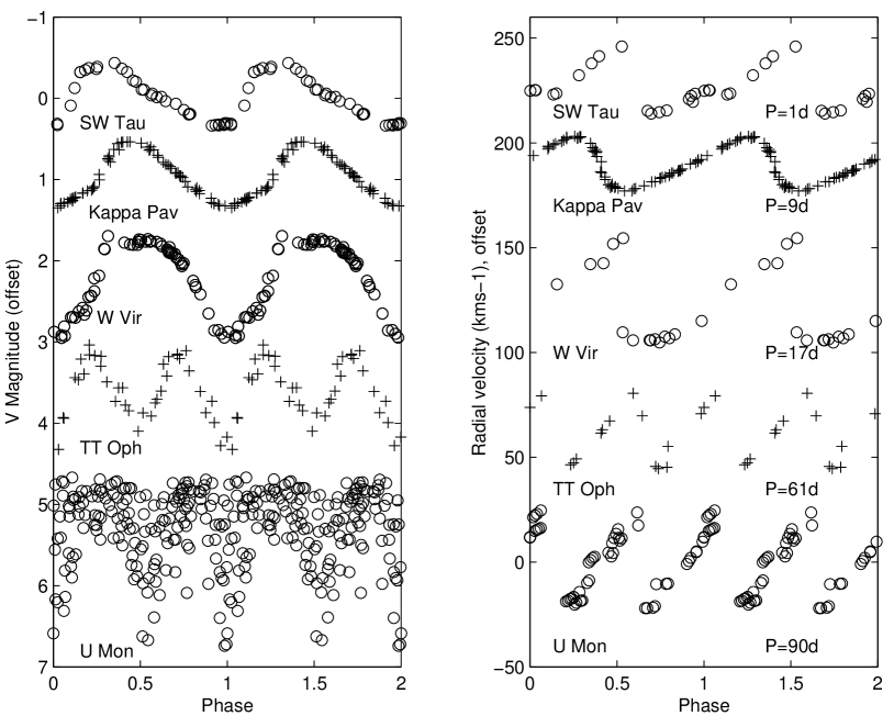
Figure 1: Photometry (left) and velocity curves (right) of selected Type II Cepheids phased using a zero point of minimum $V$ magnitude.

2 Traditional phasing

In order to be able to understand the regular pulsations of stars one needs to characterize the basic parameters of what changes over a pulsation cycle. One method is to plot the data (such as photometry or radial velocity) as a function of pulsational phase. This is shown in Figure 1 for a selection of Type II Cepheids, with periods ranging from 1.6 d (SW Tau) to 90 d (U Mon). In this, using a fixed zero point and a known period, data over a wide time interval can be compared. Traditionally, the zero point of this phasing has been based on the time of maximum (e.g. Moffett & Barnes, 1984; Schmidt et al., 2003a, b), or minimum (Pollard et al., 1996) of the star’s light curve. This is due to the historical precedent that stellar variability is generally first discovered through overall light variations. In the more regular Cepheids such as SW Tau and $\kappa$ Pav (top, Figure 1), the determination of the position of an extremum is a relatively straight-forward process. However the more complicated RV Tauri stars (i.e. U Mon, lowest curve, Figure 1), are less obvious. There is an additional problem that the phases of maximum and minimum light do not necessarily occur at the same time in different photometric filters. As such, while the extrema in the light curves represent a relatively easily observed quantity, they do not represent an optimal means by which to compare the astrophysical behaviour of the stars. Two main problems are encountered in phasing data based on maximum or minimum light. Firstly, a photometric filter region must be chosen, and secondly, the light extrema must be well defined.

The first is trivial only if all the photometry used is from a single band-pass. As soon as other band-passes are observed, the extrema do not exactly coincide because they are sampling different regions of the stellar atmosphere. This is clearly seen in Figures 2a, 3a and 4a and Table 1, where maximum light shifts to a later phase at longer wavelengths (from B to I). Astrophysically, this is due to changes in temperature and hence flux distribution over the pulsation cycle. As the stellar photosphere expands and cools, the peak flux shifts to longer wavelengths, causing maximum light in the redder band-passes to occur slightly later in the pulsation cycle. An extreme case is W Vir (Figure 4a and Table 1) in which maximum light shifts forward in phase by 0.2 of a pulsation cycle between V and R as the primary maximum becomes less prominent in the red. This maximum is most likely associated with the shock wave propagating through the star during this phase (Abt & Hardie, 1960).

The second problem, an ill-defined maximum or minimum, will depend critically on the data density obtained and the repeatability of the light curve. As with any fitting to observational data, a large scatter in the data points can introduce large errors in the extrema fitting. The broadness of the extrema can also add to the difficulty in determining the zero point. This is seen in SW Tau (Figure 2) where the minima are quite broad in all the band-passes observed. As seen from Figure 1, this represents one of the more regular stars of the sample. The scatter for U Mon is even greater and is affected by long term variations in the light curve and irregularities in the depths of the minima.

Both of these problems lead to slight shifts in the zero points between the stars, such that the same phase does not represent the same physical state for each star. It should also be noted that different stars spend a different fraction of their pulsation cycle brightening from minimum to maximum light. Hence, when basing a zero point on minimum light, the phases of maximum light compared are offset and vice versa.This can been seen in Figures 2a, 3a and 4a and Table 1, where the duration of the rise from minimum to maximum light ranges from 0.2 to 0.5 of a pulsation cycle. This leads to difficulty in comparing stars with a range of light curves at the same phases.

Table 1: Phase shifts^a (columns 2 to 9) of photometric extrema relative to minimum V light, which by definition is phase=0.0. Columns 10 and 11 are respectively the phase shift between photometric and dynamic zero points ($\Delta$) and its uncertainty (HWHM). See text (end of Section 3) for detailed explanation of these terms.

Star	$\phi_{min}$ B	$\phi_{min}$V	$\phi_{min}$ R	$\phi_{min}$ I	$\phi_{max}$ B	$\phi_{max}$ V	$\phi_{max}$ R	$\phi_{max}$ I	$\Delta\phi_{V_{min}-dynamic}$	HWHM
SW Tau	$-0.13$	0.00	$-0.12$	$-0.01$	0.21	0.35	0.36	0.37	0.07	0.09
$\kappa$ Pav	$-0.02$	0.00	$0.02$	$0.03$	0.42	0.44	0.46	0.50	0.25	0.03
W Vir	$-0.01$	0.00	$0.01$	$0.02$	0.34	0.36	0.56	0.56	0.29	0.01
TT Oph	$-0.02$	0.00	$0.01$	$0.02$	0.20	0.72	0.23	0.24	0.12	0.10
U Mon	$-0.01$	0.00	$0.02$	$0.04$	0.67	0.27	0.79	0.76	0.15	0.04

^aThe uncertainty in these phase shifts varies from star to star and between passbands. The range is from $\pm$0.07 (for V in W Vir) to $\pm$0.16 (for I in $\kappa$ Pav) when measured at 0.1 mag above the minimum (or below the maximum) of any light curve.

An alternative approach which phases the astronomical data based on the same physical state for each star is desirable.

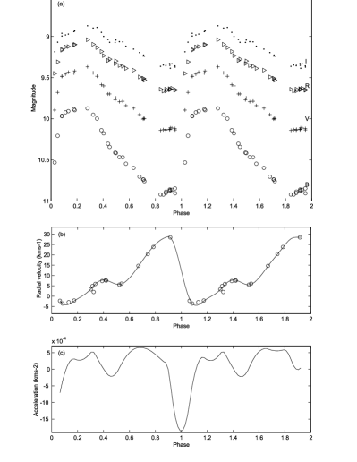
Figure 2: SW Tau (a) BVRI photometry, (b) spline-fitted mean Fe I radial velocities, and (c) acceleration curves. SW Tau is phased on a 1.58356-day period from McSaveney (2003) and using the zero point from the acceleration curve.

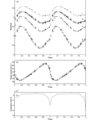
Figure 3: $\kappa$ Pav (a) BVRI photometry, (b) spline-fitted mean Fe I radial velocities, and (c) acceleration curves. $\kappa$ Pav is phased on a 9.0714-day period from McSaveney (2003) and using the zero point from the acceleration curve.

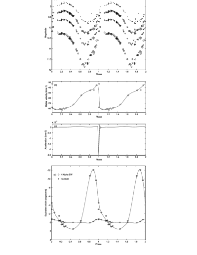
Figure 4: W Vir (a) BVRI photometry, (b) spline-fitted mean Fe I radial velocities, (c) acceleration curves, and (d) H$\alpha$ and He I equivalent widths. W Vir is phased on a 17.2768-day period from McSaveney (2003) and using the zero point from the acceleration curve.

3 Alternate phasing techniques

The pulsation cycle of a star can be observed physically in a number of ways through changes in brightness (photometry), radial velocity (spectroscopy) and angular diameter (interferometry). Having discussed the problems of using the light curves, we turn to the other techniques. Both give an indication of radii changes, though the angular diameter far more directly than the radial velocities. Maximum, mean or minimum radius would be useful as a calibration point. To date Type II Cepheids have not been observed interferometrically, so the radial velocities remain the most easily observed parameter. Ideally, one would use radial velocity curves to obtain radii changes and hence well defined zero points for phasing the data. However, this is not a straight-forward process.

Derivation of radii changes from velocity curves requires integration of the pulsational velocity curve. This differs from the measured radial velocity curve due to limb-darkening effects across the disk and the fact that the star is a spheroidal object changing in size and not a point source moving towards and away from us. This can be corrected for by the use of a geometric projection and limb darkening coefficient p, but the exact value of the coefficient varies in the literature (1.31, Hindsley & Bell (1986), 1.41, Albrow & Cottrell (1994)). As well as varying from star to star, this “constant” also varies as a function of pulsational phase, method of velocity measurement and line formation depth (Sabbey et al., 1995; Nardetto et al, 2004). These values and statements are also based on discussions of Classical Cepheids and their applicability to the Type II Cepheids is not proven. In addition, the radius derived from a particular line or species will trace the radius of that particular line formation region. Certain infra-red regions will probe deeper into the stellar photosphere and produce different radii to those determined from iron lines in the visual wavelength regions.

Minimum radius of the star has been used previously for phasing (Marengo et al., 2002) by setting the zero phase point to be the time at which the pulsational velocity moved from a positive to a negative value. This does, however, require the transformation of the radial velocity into a pulsational velocity, with the uncertainties mentioned earlier. In a more recent paper, Marengo et al. (2004) advocated dynamical phasing based on the radial velocity curve. The reasoning given was this phasing was based on hydrodynamical quantities and could thus be more readily compared with the time-dependent hydrodynamical models. These authors also discussed the phase lag observed using both the light maximum and radius minimum zero points.

Given the provisos of working with the pulsational velocities and radii, it was decided to examine the acceleration curve produced by taking the derivative of the radial velocity curve. While not the true acceleration curve, as it is not the derivative of the pulsational velocity, it is a clear indication of changes in the bulk motion of the line formation region. The minimum of this acceleration was then used, as for these stars it marked the transition between the bulk of the material in the line formation region falling inwards and moving outwards. By using the same species from the same wavelength regions, a more robust comparison of material under the same temperature and pressure conditions is obtained for the different stars. This also minimized the number of assumptions required in analyzing the data and is model independent.

In applying this technique a spline curve is fitted to the phased radial velocity curve of a particular line or species (see Figures 2b, 3b and 4b). Care is taken to fit over several repeated cycles to avoid end effects. This curve is then differentiated to find the acceleration. The minimum of this curve defines the phasing zero point, namely minimum acceleration. The data are then rephased based upon this. Figures 2c, 3c and 4c show that the acceleration minimum is far more clearly defined than the photometric minima shown in Figures 2a, 3a and 4a.

Quantitative estimates of the uncertainty of the derived dynamical zero point phase have been determined from the acceleration data, based upon the half width at half the minimum of the acceleration dip (see HWHM in Table 1). We note that it is not just dependent upon the data density around the minimum acceleration point, but also depends upon the steepness of the radial velocity curve at that point.

4 Application

To test this technique of dynamical phasing, it has been applied to a selection of Type II Cepheids. The observations are taken from McSaveney (2003). The BVRI photometry is from observations made by A.C. Gilmore and P.M. Kilmartin, using automated, single-channel photometers mounted on the Optical Craftsmen 0.61-m telescope at Mount John University Observatory (MJUO). The velocities are measured from spectra obtained by JAM, using a high-resolution spectrograph mounted on the McLellan 1.0-m telescope at MJUO. Spectroscopic data were reduced using FIGARO processes which were supplemented by MATLAB scripts.

The velocity curves shown here were obtained by averaging a selection of Fe I line velocities. These Fe I lines, with a range of excitation potentials and line strengths, represent a region of the star’s photosphere in which line formation is well understood and can be considered representative of the star. We are aware of line level effects between various species (see for example Wallerstein et al. (1992)), but in this paper we are considering only those layers representing these Fe I lines.

The individual velocities were measured by taking a mean of the line bisector velocities at depths 0.7, 0.8 and 0.9 for each line. This followed the line bisector method as developed by Albrow (1994) and used in Wallerstein et al. (1992). This was used in preference to methods using line core velocities, to smooth out any line asymmetries. These line asymmetries were outside the scope of this work (McSaveney, 2003).

The three stars shown in this paper (SW Tau – Figure 2, $\kappa$ Pav – Figure 3 and W Vir – Figure 4) constitute a representative sample of Type II Cepheids of periods ranging from 1.58 to 17.28 days. The Fe I lines from which these velocities were measured show a range of behaviour over a pulsational cycle, from little change in line width in SW Tau (the shortest period star), to mild broadening at phase 0.0 in $\kappa$ Pav, to extensive broadening and line-splitting at phase 0.0 in W Vir. As can be seen from Figures 2, 3 and 4, the dynamical phasing technique can be used on all of these stars, despite the differences in velocity curve produced by the different line behaviours.

The acceleration curves shown for each star (Figures 2c, 3c and 4c) all have distinct minima that have been rephased to 0.0. Even in the case of SW Tau, where a second minimum is found around phase 0.4–0.5 due to a bump in the velocity curve, this is easily distinguished from the primary velocity field reversal.

The result of this phasing provides a much easier comparison between these stars, as it is clear when the motions of the velocity fields are reversing. In contrast, by phasing using V minimum (Figure 1), it occurs between phase 0.85 and 0.95 in SW Tau, at $\sim$0.8 for $\kappa$ Pav and $\sim$0.7 in W Vir. These are shown quantitatively in Table 1, where the phase shifts between V minimum and dynamical zero points ($\Delta$) are given for the five Type II Cepheids in our sample. These $\Delta$s show that there is more than 0.2 in phase difference between these values that is not related in any way to a physical stellar parameter. Also the dynamical zero points have a much better defined position (HWHM in Table 1 is between 0.01 and 0.10) when compared to the uncertainties in the photometric zero points, which range from 0.07 to at least 0.16 and vary considerably from passband to passband for a given star. This effect is also clearly visible in Figures 2, 3 and 4, where the width (in phase) of the acceleration minimum for a given object is in all cases much narrower than any of its respective photometric passband minima.

Astrophysically, this shows that the dynamical zero point provides a clear common phase compared to that indicated by any particular photometric bandpass. The dynamical zero point indicates when the direction of motion of the line formation region shifts from falling inwards to moving outwards. In these stars, this is when shock-wave features are detected as a shock propagates through the line forming regions. Hence spectral features such as line broadening, splitting and emission all occur around this phase. This is seen in the H$\alpha$ and He I equivalent widths (see Figure 4d) where the strongest emission occurs at around phase 0.0. This is also observed in a wider range of Type II Cepheids (McSaveney, 2003).

5 Discussion

There are several assumptions which will have an affect on the results obtained when using this technique. These include what line species are used, the method of measuring the radial velocities and how the spline curve is fitted.

An important point to note with this technique is that different line species are formed over slightly different regions of the stellar photosphere, and will therefore give slightly different zero points. While this may be construed as a problem as large as that of the shifts in zero point from the photometry, this is not actually the case. The spectral line formation regions can be far more specifically defined than the far broader photometric regions, particularly for the dominant species (usually Fe I), from which the velocities are determined. When establishing the velocities care should be taken to use lines of similar species, excitation potential and log(gf) such that there is a high degree of confidence that the lines are formed in the same region of the stellar photosphere. Averaging H$\alpha$ velocities with Fe I velocities would be counterproductive given the large phase lags and amplitude differences observed between these lines in Type I and Type II Cepheids (Wallerstein et al., 1992; Vinko et al., 1998; Petterson, 2002; McSaveney, 2003).

The radial velocity measuring technique will also affect the velocity determined. Techniques fitting to the sides of the lines, or taking the line bisector value from midway up or higher (closer to the star’s continuum) in the line, will be more easily distorted by line broadening or splitting. This will result in different amplitudes. Techniques fitting to the line bisector from deeper in the line core (as used in this work) give a better indication of the maximum and minimum velocities achieved by material in the line forming regions. The crucial point is to be consistent in the manner of application such that it is clear that the stars (as shown by the appropriate spectral lines) show the same measured zero-point behaviour.

As with any data set, good radial velocity phase coverage is essential, particularly at the critical phases between minimum and maximum light when the minimum radius occurs. To avoid distortion by end effects in the spline fitting, repetition of the full velocity curve is required. This technique is quite data intensive. However, for the comparison of stars with a range of periods all with large datasets, it is invaluable.

6 Conclusion

Using the acceleration changes as a zero point in dynamical phasing offers a substantial improvement over previous phasing techniques in understanding the pulsations in Type II Cepheids. It shifts the phasing emphasis from the more ambiguous light extrema to the astrophysically more specific, yet still observable, changes observed through radial velocity curves. This allows a better understanding of the physics of the stellar pulsations and clearer comparison between stars, as they can be collectively phased to a more clearly defined astrophysical state.

This technique has been applied to a selection of Type II Cepheids and found to work extremely well for a variety of velocity curve shapes and periods. From a preliminary survey of SW Tau, $\kappa$ Pav and W Vir, it is clear that the shock-associated features of line broadening and line splitting, and H$\alpha$ and He I emission, are associated with the bulk motion reversal observed and can be more clearly compared by using this particular zero point. More detailed study of the shock behaviour for a wider range of Type II Cepheids using this technique can be found in McSaveney et al. (2005, in preparation).

References

- Abt & Hardie (1960) Abt H.A., Hardie R.H., 1960, ApJ, 131 155
- Albrow (1994) Albrow M.D., 1994, PhD thesis, University of Canterbury
- Albrow & Cottrell (1994) Albrow M.D., Cottrell P.L., 1994, MNRAS, 267, 548
- Hindsley & Bell (1986) Hindsley R., Bell R.A., 1986, PASP, 98, 881
- Marengo et al. (2002) Marengo M., Sasselov D.D., Karovska M., Papaliolios C., Armstrong J.T., 2002, ApJ, 567, 1131
- Marengo et al. (2004) Marengo M., Karovska M., Sasselov D.D., Sanchez M., 2004, ApJ, 603, 285
- McSaveney (2003) McSaveney J.A., 2003, PhD thesis, Univ. of Canterbury
- Moffett & Barnes (1984) Moffett T.J., Barnes T.G., ApJS, 55, 389
- Nardetto et al (2004) Nardetto N., Fokin A., Mourard D., Mathias Ph., Kervalla P., Bersier D., 2004, A & A, 428, 131
- Petterson (2002) Petterson O., 2002, PhD thesis, University of Canterbury
- Pollard et al. (1996) Pollard K.R., Cottrell P.L., Kilmartin P., Gilmore A., 1996a, MNRAS, 279, 949
- Sabbey et al. (1995) Sabbey C.N., Sasselov D.D., Fieldus M.S., Lester J.B., Venn K.A., Butler R.P., 1995, ApJ, 446, 250
- Schmidt et al. (2003a) Schmidt E.G., Lee K.M., Johnston D., Newman P.R., Snedden S.A., 2003, AJ, 126, 906
- Schmidt et al. (2003b) Schmidt E.G., Langan S., Lee K.M., Johnston D., Newman P.R., Snedden S.A.. 2003, AJ, 126, 2495
- Vinko et al. (1998) Vinkó J., Evans N., Kiss L., Szabados L., 1998, MNRAS, 296, 824
- Wallerstein et al. (1992) Wallerstein G., Jacobsen T.S., Cottrell P.L., Clark M., Albrow M., 1992, MNRAS, 259, 474