Measurement of Pressure Dependent Fluorescence Yield of Air: Calibration Factor for UHECR Detectors

Abstract

In a test experiment at the Final Focus Test Beam of the Stanford Linear Accelerator Center, the fluorescence yield of 28.5 GeV electrons in air and nitrogen was measured. The measured photon yields between 300 and 400 nm at 1 atm and 29^∘C are

$$Y(760~{}{\rm Torr})^{\rm air}=4.42\pm 0.73{~{}~{}~{}\rm and~{}~{}~{}}Y(760~{}{\rm Torr})^{\rm N_{2}}=29.2\pm 4.8$$

photons per electron per meter. Assuming that the fluorescence yield is proportional to the energy deposition of a charged particle traveling through air, good agreement with measurements at lower particle energies is observed.

1 Introduction

Measuring the energy spectrum of Ultra High Energy Cosmic Rays (UHECR) is the goal of several past, present, and future experiments using the air fluorescence technique. It is of special interest to measure the spectrum in the range of $10^{20}$ eV and establish whether it is suppressed as predicted by the GZK mechanism [1]. The published results of the two, at that time largest, experiments collecting UHECR data disagree [2]. One of those detectors, the High Resolution Fly’s Eye (HiRes) utilizes air fluorescence to detect cosmic rays and to determine their energy. The other experiment, the Akeno Giant Air Shower Array (AGASA), a ground array of scintillation counters in Japan, used the particle sampling technique. The energy dependent HiRes flux measurement is systematically smaller than that of AGASA and is consistent with a GZK suppression. One systematic uncertainty in the case of the fluorescence technique is the uncertainty of the measured fluorescence yield of charged particles in air itself. A more precise study of the yield would be valuable in seeking the cause for the apparent discrepancies between the techniques.

There are a number of previous fluorescence yield experiments. In his thesis from 1967 Bunner summarized the existing data and quoted uncertainties of around 30% on the reported fluorescence efficiencies [3]. Bunner’s work served as the standard reference for fluorescence technique based cosmic ray experiments into the nineties. In a more recent experiment [4], Kakimoto et al. measured the total fluorescence yield between 300 and 400 nm with an uncertainty of $>$10% and the yield at three pronounced lines - 337 nm, 357 nm, and 391 nm. The newest measurements using a ${}^{90}\mathrm{Sr}~{}\beta$ source published by Nagano et al. [5, 6], determined the total fluorescence yield between 300 nm and 406 nm with a systematic uncertainty of 13.2% as the sum of the yields of 15 wave bands which were measured separately using narrow band filters. An improvement in the present level of accuracy and confidence is necessary, from measurements not subject to the same set of systematic uncertainties, especially since other systematics, like the atmospheric uncertainty, which depends on variable pressure profile, transparency, scattering, etc., are expected to be reduced significantly in the near future.

New experiments using the fluorescence technique are beginning to take data, are in construction, or are being planned. These include the hybrid detectors of the Pierre Auger Observatory [7], and of the Telescope Array (TA) [8], or the space-based fluorescence detectors EUSO [9] and OWL [10]. These experiments are designed to increase the detection aperture and statistics in the ultra high energy region. The hybrid detectors should also help to resolve the disagreements between the particle sampling technique and the fluorescence technique. Independent measurements of the fluorescence yield of charged particles in air as presented in this paper, and refinements proposed to follow this work, will complete the picture.

The test experiment presented in this paper, T-461, was conducted at the Stanford Linear Accelerator Center (SLAC) to study the feasibility of a larger fluorescence experiment, FLASH. Both experiments have since been installed in SLAC’s Final Focus Test Beam (FFTB) tunnel. FLASH aims to measure the net fluorescence yield as well as the yields of the individual spectral lines with a systematic uncertainty of less than 10%. Measurements with mono-energetic electrons, and separately with electron-positron showers downstream of thick materials, are used to measure the fluorescence yield down to an electron energy of 100 keV[11]. T-461 used only the mono-energetic beam approach and was designed to measure the total fluorescence yield between 300 and 400 nm using a UV bandpass filter as installed in the HiRes experiment. In the following Section, the experimental setup of T-461 will be described in detail. In Section 3, the selection of good quality data is described. This is followed by a brief description of the calibration of the experimental setup in Section 4. The fluorescence yield measured in air and nitrogen is presented in Section 5 along with a list of the systematic errors which were studied. In the last Section, the T-461 results are compared with previous measurements and improvements are discussed for the full scale fluorescence experiment FLASH.

2 Experimental setup

The experiment T-461 was carried out in the Final Focus Fest Beam at SLAC. It was installed in an air gap of the beam pipe, approximately 35 cm long, downstream of the dump magnets. The beam is focused effectively at infinity in this region, so that the bremsstrahlung from the beam windows and thin experimental equipment in this region continues along the electron beam to the dump. In addition, since the thickness of the material in the beam was held below 1% of a radiation length, multiple scattering of beam particles into downstream collimators is negligible.

A beam spot size of about 2$\times$1 mm was generated in this region, with intensities between $10^{9}$ and 2 $\times 10^{10}$ e^-/pulse. Between $10^{8}$ and $10^{9}$ electrons per pulse, the intensity is below the sensitivity of the beam position monitors and feedback becomes inoperative. Nonetheless, intensities as low as $10^{8}$ were delivered for 24 hours during T-461. However, the beam current measuring toroidal ferrite-core current transformer registered intensity variations of $\approx$ 30% during this period. The toroid was calibrated using charge-injection on a one-turn winding. The accuracy was determined to be 10% for beam charges below 10⁹ e^- by cross comparison with a high-accuracy toroid during a subsequent FLASH run.

The thin target installed in FFTB during T-461 was a 1.6 liter air-filled cylinder, coaxial with the beam. The vessel had thin beam windows and radial ports to allow light to reach shielded photomultiplier tubes (PMTs) as shown in Figure 1. The inside of the vessel was black-anodized and baffled to suppress all but direct light from the beam. The fluorescence light was detected in two independent radial tubes. In each, the optical aperture was defined by a slit near the beam axis, measured to be 1 cm parallel, and 1.7 cm perpendicular to it. In each tube, light passed through a series of circular apertures forming a baffle. At the far end of the 42.9 cm long baffle, the PMTs were protected from scattered background radiation by using dielectric mirrors to reflect the fluorescence light through 90⁰ into the detector. There, the PMTs were encased in a lead vault. As can be seen in Figure 1, a UV band pass filter from the High Resolution Fly’s Eye (HiRes) experiment was installed between the dielectric mirror and PMT. The PMTs, Philips (now Photonis) XP3062/FL, are also the type used in the HiRes experiment. The optical unit including the mirror, UV filter, and PMT was calibrated at the University of Utah after T-461 data taking was completed.

Figure 1: The experimental setup showing one of two orthogonal optical pathways through baffled channels, and 45 degree reflection to a photomultiplier tube (PMT). The values are given in inches [mm].

To monitor the stability of the PMT response in-situ, ultraviolet LEDs were installed on arms opposite the detector arms. The LEDs were fired between beam pulses emitting light across the fluorescence cylinder. To measure beam induced backgrounds in the PMTs, optically hooded — “blind” — PMTs were mounted beside the “live” tubes. Signals of the blind tubes were collected continuously along with the signals of the live tubes and normalized to the live signals by collecting data while the fluorescence chamber was filled with a non-fluorescing gas.

The gas system allowed the flow of a premixed gas with a pressure in the vessel between 3 and 760 Torr. The pressure was set manually, but monitored by computer during data taking. Data for dry air and pure nitrogen were collected with flowing gas. Data for various air-nitrogen mixtures were collected without flowing the gas through the chamber.

During T-461, a CAMAC based DAQ system was used to collect the data. Pulse amplitudes from the PMTs and the beam toroid signal were recorded using LRS 2249W ADCs from Lecroy. PMT high voltage, pressure and temperature were digitized with the Smart Analog Module, a 32-channel module used to digitize analog signals.

3 Data taking and event selection

Altogether about 1 million events were recorded with a mean high voltage of 1186 V supplied to the PMTs. The voltage was constrained to better than half a volt over the entire run period.

Throughout the data taking, a special trigger, about once every 52 beam pulses, was used to measure ADC pedestals. The pedestal values were found to be stable around 45 and 47 counts for the north and south signal PMTs, respectively. From each beam event the nearest pedestal measurement was subtracted.

The PMT response was tracked throughout the data taking with ultraviolet LEDs. As for the pedestal events, LED events were also taken once every 52 beam events. The response of the south PMT to the LED was very stable (around 2%) during the experiment as seen in Figure 2a. Similar to the pedestal subtraction scheme, each beam induced event was assigned the closest LED reading.

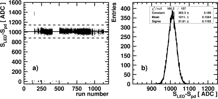
Figure 2: Pedestal subtracted response of the south signal PMT to the LED. a) The south PMT response versus the run number. The dashed lines represent the data quality preselection cut. b) The projection of the response onto the signal axis.

In order to remove poor quality data and data with unstable detector response, the LED data of the south PMT were fitted to a Gaussian, see Figure 2b. Beam data during time periods where LED events were outside of $\pm 6\sigma$ of the fitted mean were removed from the data set. The $\pm 6\sigma$ band is represented by two dashed lines in Figure 2a. Less than 1.5% of the data were excluded by this requirement (see Table 1).

Cut	Efficiency (%)
LED requirement	98.6
PMT correlation	98.5
Beam distribution	84.7
Linearity cut	41.9
Air	15.8
Mixtures	13.7
N2 (flowing)	2.6

Table 1: Efficiency of the main preselection requirements imposed on the T-461 data. See Section 3 for details.

Figure 3 shows that the north PMT’s response was unstable, probably due to a HV connector problem. While the north PMT data were used to check the data quality, because of such wide systematic wandering, the north PMT was not used in the final result. The pedestal subtracted LED signals were used to correct for gain changes shown in Figures 2 and 3 by the formulas,

$$S_{cd}=\left(S-S_{pd}\right)\times\frac{\langle S_{LED}\rangle}{S_{LED}-S_{pd}}$$ (1)

and

$$N_{cd}=\left(N-N_{pd}\right)\times\frac{\langle N_{LED}\rangle}{N_{LED}-N_{pd}}.$$ (2)

Here, $S_{cd}$ and $N_{cd}$ are the stability corrected and pedestal subtracted south and north PMT signals, $S$ and $N$ are the raw ADC readouts from the PMTs, $S_{pd}$ and $N_{pd}$ are the signals of the assigned pedestal events, $\langle S_{LED}\rangle$ and $\langle N_{LED}\rangle$ are the fitted means of the pedestal subtracted LED distributions shown for the signal PMTs by horizontal lines in Figure 2a and 3, and $S_{LED}$ and $N_{LED}$ are the signals of the closest LED events. The mean for all the LED events collected by the south signal PMT is $\langle S_{LED}\rangle=1011$ counts. The mean of $\langle N_{LED}\rangle=765$ counts was calculated only from the longest period of north PMT gain stability which occurred between runs 504 and 947.

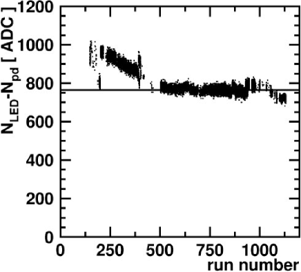
Figure 3: Pedestal subtracted response of the north signal PMT to the LED. The $x$-axis is the run number and the $y$-axis is the pedestal subtracted LED signal.

After the PMT signals had been corrected for LED response the signal size was required to correlate well between the two signal PMTs. In Figure 4a the corrected signal, $N_{cd}$, of the north PMT is plotted versus the corrected signal, $S_{cd}$, of the south PMT. A strong correlation for most of the data is quite apparent. The data were fitted to the linear function $N_{cd}=kS_{cd}$, $k$ being the correlation factor of the two signals. Then the axes were rotated so that the fitted line was the ordinate of a new plot. The new abscissa is calculated according to the formula $x=N_{cd}\cos\theta-S_{cd}\sin\theta$, where $k=\tan\theta$. The rotated distribution was then projected onto the new abscissa. The resulting distribution is shown in Figure 4b. All events beyond $\pm 85.0$ ADC counts were removed from the data sample. The upper and lower lines in Figure 4a represent the 170 ADC counts acceptance band. The fraction of events remaining after this cut is listed in Table 1.

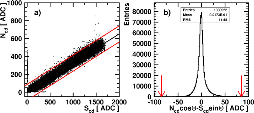
Figure 4: Signal PMT correlation. a) The $x$-axis is the background subtracted and gain corrected south PMT signal and the $y$-axis is the background subtracted and gain corrected north PMT signal. Air, N₂, and air-N₂ mixture events are shown. The dashed lines correspond to the PMT correlation cut, see Table 1. b) Projection of the rotated distribution showing the correlation between $N_{cd}$ and $S_{cd}$ where $x=N_{cd}\cos\theta-S_{cd}\sin\theta$. See text for details.

During the two weeks of data collection, data were recorded at beam charges between $10^{8}$ and $10^{10}\ e^{-}$ per bunch. For each data part, the target beam charge was specified, and the charge of each bunch was measured with a toroid installed up-stream of the thin target vessel. Figure 5 shows example distributions of measured beam charges for four runs. As can be seen, some of the distributions, especially those with low beam intensity, have long tails possibly indicating poor beam quality. To remove the corresponding events from the data sample, the beam charge distribution of each run was fitted to a Gaussian curve and events lying outside of 2$\sigma$ were cut. The selection efficiency of this requirement is also listed in Table 1.

Figure 5: The beam charge distributions of four typical data runs as measured by an upstream toroid during T-461.

In order to investigate possible background due to reflected Cherenkov light or other sources, some data were collected while the gas chamber was filled with ethylene, a non-fluorescing gas. The same range of pressures were investigated as for air and nitrogen. The corrected signals, $N_{cd}$ and $S_{cd}$, of both PMTs for the ethylene data runs are plotted versus pressure in Figure 6. The figure shows that $S_{cd}$ and $N_{cd}$ do not depend on the pressure, indicating negligible light background. The larger signal values for each signal tube at the lowest pressure probably indicate the presence of a trace amount of air.

Figure 6: “Blind” – $s-s_{pd}$, $n-n_{pd}$ – and “signal” – $S_{cd}$, $N_{cd}$ – PMT signals for ethylene at different pressures. a) The data taken by the south PMTs and b) the north PMT data. The relative difference between the ADC values illustrates the differences in gains between corresponding signal and blind PMTs.

During the entire experiment, the beam related background was measured by two “blind” PMTs positioned next to the “signal” PMTs. Figure 7 shows that the blind PMT signal increases with the beam charge. Using the ethylene data the blind PMT data was normalized to the signal PMT data. The pedestal corrected signals of the blind PMTs are also plotted in Figure 6. As can be seen, signal and blind PMTs track each other well. The relative difference between the values illustrates the differences in gains between the signal and the blind PMTs. The mean ratios $\langle S_{bg}\rangle=1.22$ and $\langle N_{bg}\rangle=0.65$ are used for the beam related background subtraction:

$$S_{fl} = S_{cd}-\langle S_{bg}\rangle(s-s_{pd})$$ (3)

and

$$N_{fl} = N_{cd}-\langle N_{bg}\rangle(n-n_{pd}),$$ (4)

where $S_{fl}$, $N_{fl}$ are the background subtracted and LED corrected fluorescence signals in ADC counts, $s$, $n$ are the corresponding blind PMT signals, and $s_{pd}$, $n_{pd}$ are the assigned pedestal measurements for the blind photo tube channels.

Figure 7: The south background PMT signal versus the number of beam electrons per bunch.

During the run a non-linear enhancement of the fluorescence signal with respect to the beam charge was observed. This effect was seen in both pure nitrogen and air. This non-linearity is most likely caused by the acceleration of secondary electrons in the very strong radial electric field of the picosecond long beam pulse of relativistic electrons. This effect has, for example, been studied in [12]. For the purpose of measuring the fluorescence yield per electron, it is necessary to remove all data which were taken in the non-linear beam charge range. In order to define an upper limit on the beam charge linear fits to the fluorescence signals $N_{fl}$ and $S_{fl}$ versus beam charge were performed for varying beam charge ranges. Based on the quality of the fits an upper limit of $1\times 10^{9}e^{-}$ per beam pulse was chosen and all the data taken at higher beam charges were removed from the data sample. Two example fits with an applied beam charge limit of $1\times 10^{9}~{}e^{-}$ per pulse are shown in Figure 8.

Figure 8: Stability corrected and background subtracted signal versus the number of electrons per beam pulse for two selected pressure regions for air.

The final fraction of events remaining after all cuts for air, nitrogen and nitrogen-air mixtures are listed in Table 1. In the case of nitrogen, only data which were collected when the gas was flowing through the chamber were considered. This ensured that potential impurities from small leaks of ambient air in the chamber were negligible. The fluorescence yield $Y$ per electron per meter in air and nitrogen was then determined based on these preselected data samples as will be described in the following sections.

4 Calibration and Geometrical Acceptance

Before the fluorescence yield can be calculated, the detectors and the DAQ system need to be calibrated and the geometrical acceptance of the detectors, as they were mounted on the thin target chamber, must be determined.

The fluorescence yield then can be calculated as

$$Y=\frac{1}{N_{e^{-}}}\cdot\frac{S_{fl}\cdot C}{R_{D}\cdot G},$$ (5)

where $S_{fl}$ is the background subtracted and LED corrected fluorescence signal in ADC counts, $C$ is the calibration factor converting ADC counts into pC, $N_{e^{-}}$ is the number of electrons in a beam pulse, $G$ is the effective geometrical acceptance in m^-1, and $R_{D}$ is the photon flux responsivity of the detector assembly in pC m²/$\gamma$.

As mentioned in the last section only the south signal PMT was used for the final result. The calibration constant $C$ for its DAQ channel was measured to be 1/3.48 pC/ADC counts.

The south detector assembly was calibrated after T-461 data taking was completed. As can be seen in Figure 1, the PMT was mounted in a brass housing along with a HiRes filter and a mirror. The complete unit was calibrated in a standard HiRes calibration setup at the University of Utah. A schematic of the calibration setup is shown in Figure 9. It consisted of a 100 W high-pressure mercury arc lamp, a monochromator, a light guide and a diffuser as the light source, a 1.8 m light path in a baffled foam tube, and a stand with a calibrated silicon photo diode installed next to the south PMT unit. The diffuser, the baffled light path, the Si photo diode and the PMT unit were enclosed completely in a dark box. The south signal PMT detector unit and the silicon photo diode were aligned so that they were directly facing the diffuser. During calibration the monochromator scanned the wavelength region between 260 nm and 420 nm in 1 nm steps. After several monochromator scans were recorded, the PMT and photo diode were swapped. In this manner light emitted by the mercury lamp was collected by the PMT assembly and the diode. The current output of each detector was measured by a pico ampere meter. From the calibration curve of the wavelength dependent responsivity of the silicon photo diode in units of A/(W/$\mathrm{cm^{2}}$), and the measured size of the entrance pupil of the T-461 detector assembly, its responsivity could be calculated in units of A/(W/$\mathrm{cm^{2}}$). In order to calculate the spectrum weighted photon flux responsivity $R_{D}$ of the detector the wavelength dependent responsivity was folded with the normalized fluorescence spectrum of air and nitrogen at 760 Torr as reported in Tables 1 and 2 of reference [6]. The fluorescence photon flux responsivity between 300 and 400 nm was found to be $R_{D}=1.47\times 10^{-6}\mathrm{pC\cdot m^{2}}/\gamma$ for air and $R_{D}=1.66\times 10^{-6}\mathrm{pC\cdot m^{2}}/\gamma$ for nitrogen.

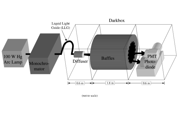
Figure 9: The detector calibration setup.

The geometrical acceptance $G^{\prime}$ was calculated as

$$G^{\prime}=\frac{W}{4\cdot\pi\cdot(D-L)\cdot D}$$ (6)

where $D$ is the distance from the beam axis to the detector unit’s aperture, $L$ is the distance from the beam axis to the slit, and $W$ is the slit width defining the beam length seen by the detector. $D$, $L$, and $W$ were measured for the south signal PMT arm and based on the measured numbers $G^{\prime}$ was calculated to be 1/213.8 m^-1. A small fraction of the energy deposited by the beam in the gas was outside the transverse aperture of the optical slit ($\pm$ 0.85 cm). This was evaluated from the Monte Carlo simulations of the process, leading to a correction of 7% and an effective geometrical acceptance of

$$G=G^{\prime}\cdot l,$$ (7)

where $l$ is $\sim$ 93% with a very small pressure dependence.

5 Resulting Fluorescence Yield

Figure 10 shows the calculated yield in units of $\frac{\gamma}{\rm e^{-}m}$ versus the measured pressure in Torr for air and nitrogen at 29${}^{\circ}\>$C. For air, the curve plateaus at about 4.4$\frac{\gamma}{\rm e^{-}m}$, while the N₂ curve continues to climb with pressure and reaches a yield approaching seven times that at 800 Torr. Figure 11 shows the measured pressure dependent yield of four different air-$\rm N_{2}$ mixtures framed by the $\rm N_{2}$ and air yield curves. Inspired by the fluorescence yield studies in previous publications [3, 5, 6], where fits were performed to the measured pressure ($p$) dependent yields of individual spectral lines, the function

$$Y(p)=\frac{C}{\frac{1}{p^{\prime}}+\frac{1}{p}}$$ (8)

was fitted to the air and N₂ yield curves using the log likelihood method with $C$ and $p^{\prime}$ as freely variable parameters. In the case of an individual spectral line, $p^{\prime}$ is the reference pressure specific to the line and $C$ is the product

$$C=\frac{dE}{dx}\cdot\frac{1}{RTh\nu}\cdot\Phi^{0}.$$ (9)

Here $dE/dx$ is the energy deposited by an electron traveling through the gas target, $R$ is the specific gas constant, $T$ is the temperature, $h\nu$ is the photon’s energy, and $\Phi^{0}$ is the fluorescence efficiency of the corresponding spectral line in the absence of collisional quenching [3, 5, 6]. The values for $p^{\prime}$ derived from the fits are 8.9 $\pm$0.8 Torr for air and 103$\pm$10 Torr for nitrogen. The functions, $Y(p)$, resulting from the fits were then used to calculate the yields in air and nitrogen at 1 atm:

$$Y(760~{}{\rm Torr})^{\rm air}=4.42\pm 0.73\frac{\gamma}{\rm e^{-}m}$$

and

$$Y(760~{}{\rm Torr})^{\rm N_{2}}=29.2\pm 4.8\frac{\gamma}{\rm e^{-}m}.$$

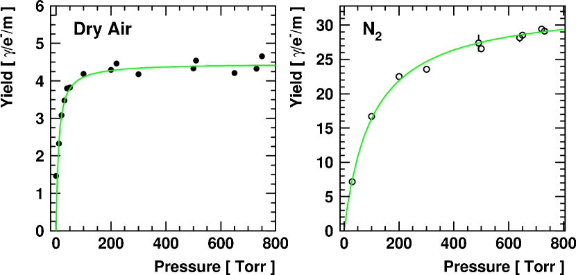
Figure 10: The fluorescence yield curves for air (left plot) and N₂ (right plot) as measured by the south PMT. The $x$-axis is the pressure measured in Torr, and the $y$-axis is the resulting fluorescence yield between 300 and 400 nm in photons per electron per meter ($\frac{\gamma}{\rm e^{-}m}$).

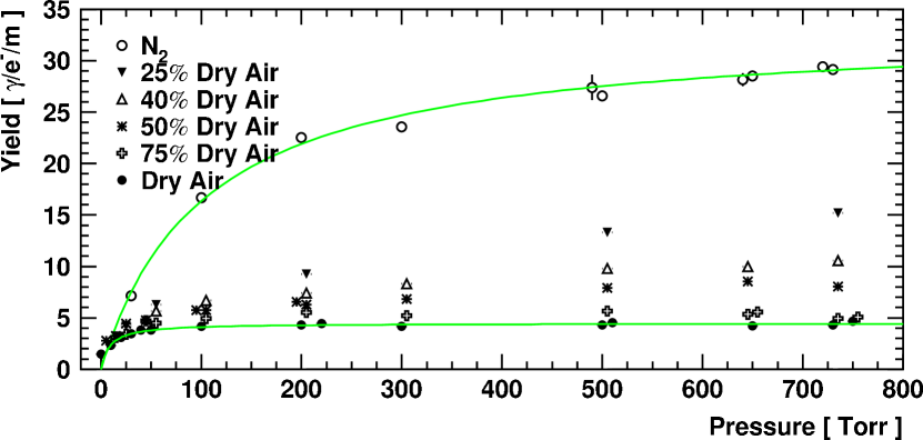
Figure 11: The fluorescence yield curves of air and N₂ and various air-N₂ mixtures. The $x$-axis is the pressure measured in Torr, and the $y$-axis is the resulting fluorescence yield between 300 and 400 nm in $\frac{\gamma}{\rm e^{-}m}$.

The sources contributing to the overall uncertainty are summarized in table 2. The total uncertainty is 16.6%. The statistical uncertainty contributes less than 1% to the total uncertainty. The largest systematic uncertainty is associated with the detector calibration (10.5%). This accounts for the transfer uncertainty from the calibration setup in Utah to SLAC, the radiometer calibration uncertainty of the silicon photo diode, in addition to statistical, environmental, geometrical, and other systematic uncertainties derived from a series of calibration measurements. The uncertainties of the fluorescence spectrum in air and nitrogen quoted in Table 1 and 2 of reference [6] were also taken into account. The second largest contribution of 10% to the total uncertainty is from the beam charge measurement. It was estimated based on systematic studies comparing simultaneous measurements of the two different toroids used during T-461 and FLASH (E-165). The uncertainty of the effective geometrical acceptance, $G$, of 7% is due to a conservative estimate of the uncertainties on the measured slit widths and the measured distances to the beam line. A potential systematic effect from the linearity cut described in Section 3 was also investigated. The linearity requirement was varied between $N_{e^{-}}<0.5\cdot 10^{9}$ and $N_{e^{-}}<1.1\cdot 10^{9}$ electrons per bunch resulting in differences of the measured yield in air and nitrogen of up to 3%. The uncertainty of the ADC calibration of the south PMT DAQ channel contributes 2% to the overall uncertainty. The smallest systematic uncertainty of 1% is associated with the background subtraction.

Relative error at 760 Torr		Air and N2
Statistics		$<<$1%
Systematics
Detector calibration	$R_{D}$	10.5%
Beam Toroid Calibration	$N_{e^{-}}$	10%
Geometrical Acceptance	$G$	7%
Linearity cut	$S_{fl}/N_{e^{-}}$	3%
ADC calibration	$C$	2%
Background subtraction	$\langle S_{bg}\rangle$	1%
Total	$Y$	16.6%

Table 2: Summary of statistical and systematic uncertainties in the measurement of the total fluorescence yield, $Y$, in air and pure nitrogen at 760 Torr at 29${}^{\circ}\>$C.

6 Fluorescence Decay Time

The strong saturation of the fluorescence yield in the pressure range up to atmospheric (Fig. 10) is caused by collisional de-excitation of the nitrogen molecules. This statistical process enforces exponential decay times on the excited states. The basic formalism is the same as in the previous section and in terms of decay lifetimes, $\tau$, may be given as $\tau=\tau_{0}/(1+p/p^{\prime})$. Here $p^{\prime}$ is the same as in eq. 8 and $\tau_{0}$ is the decay time in the absence of collisions, for example at very low pressure.

Most of the wavelengths in this study are transitions in the second positive bands, and may be expected to have similar decay properties. The 1N transition at 391 nm may be different, but accounts for a small fraction of the light at our pressures. In this experiment, decay effects are averaged over the detected wavelengths.

An overall dependence of the decay time on pressure was indeed observed. As a way of studying it, photomultiplier pulse profiles were recorded at various gas pressures, using a digital oscilloscope. Typically 16 pulses were averaged. The dependence of decay time on pressure was very obvious, as is illustrated by the pulses shown in Fig. 12 for air at 5 and 748 Torr.

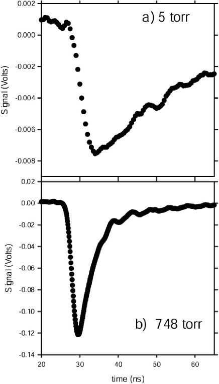
Figure 12: Pulse profiles from the photomultiplier for air pressures of 5 and 748 Torr.

In order to process the data, the small effect of beam induced background in the PMT was removed. As described in Section 3, this was accomplished by using pulse shapes recorded while the test vessel was filled with ethylene, corresponding to that part of the signal not from the gas fluorescence. Suitably normalized to the correct beam intensity, this was subtracted, sample by sample, from the fluorescence pulse profiles. The effect was noticeable only below 30 Torr, and especially in air which gives smaller signals.

The next step was to record the PMT intrinsic pulse shape, which was measured using an Sr⁹⁰ source to make picosecond long pulses of Cherenkov light in the tube face. For computational purposes, this shape was parametrized by a well fitting asymmetric probability distribution, Pearson IV [13]. (Other functions would have fitted almost as well.) The intrinsic shape was then folded with hypothetical light pulses which turned on instantly (corresponding to the SLAC picosecond electron pulse length) but decayed exponentially. The folding was repeated for a range of decay times of the light, and, for each case, the width of the folded pulse at half maximum (FWHM) was taken to characterize the pulse shape.

Using this calibration, the measured FWHM values of the actual data pulse profiles were transformed to the light decay times. Values for air and nitrogen are shown in Fig. 13. The nitrogen data below 30 Torr were excluded because of uncertainty about the effect of a small air leak in the system. Uncertainties at each point were estimated for the FWHM measurements and the background subtraction, and scaled, after fitting, so that $\chi 2$ was equal to the number of degrees of freedom. Fitting to the functional form above allows us to obtain the values for decay times at “zero pressure” (i.e. in the absence of collisional de-excitation) of $32.0\pm 2.2$ ns for air and $26.1\pm 1.2$ ns for nitrogen. At atmospheric pressure, the values found are $0.41\pm 0.01$ ns for air, and $2.20\pm 0.06$ ns for nitrogen. The values for p’ are $9.9\pm 0.7$ Torr for air and $70\pm 4$ for nitrogen. The nitrogen value is significantly lower than that obtained from the yield curve. This may be related to our assumption that all the emission lines can be treated by a single average parameter. Differences between them would distort the decay time and yield fits differently, especially given the extrapolation below 30 Torr. In future work we intend to measure the lines separately.

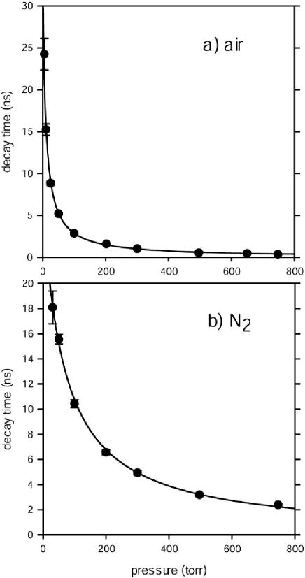
Figure 13: Decay time vs. pressure: a) air; b) nitrogen.

In the case of nitrogen, numerous measurements of the “zero pressure” decay lifetimes have been reported for various wavelength bands, mostly after excitation by proton beams. Results, summarized by Dotchin et al. [14], show values in the range 34 to 48 ns. A measurement at $10^{-6}$ Torr observed 58 ns [15]. Recently, however, Nagano and collaborators [5], using electrons to excite the nitrogen, report lower values. They give values in six wavelength bands, approximately covering the spectral range of our data. To allow a comparison between the two experiments, we have weighted the decay time for each of Nagano’s wavebands by its relative intensity and taken a weighted average. Their average value for nitrogen is then $27.4\pm 1.4$ ns. A similar average of their results for air is $30.5\pm 2$ ns. Our life time measurements agree well with Nagano and collaborators, but not with the earlier proton beam experiments.

7 Conclusion and Discussion

Figure 14 shows the total fluorescence yield between 300 and 400 nm per electron in air at 760 Torr and 29⁰C calculated in this paper as well as the yields reported by Kakimoto [4] and Nagano [6]. The yields are plotted versus the energy of the electrons injected in a thin air target and together with two dE/dx curves. The line shows the energy loss of electrons in air as calculated based on reference [16], while the dashed line represents the energy deposit of an electron in a 1 cm thick slab of air as calculated by GEANT 3 [17]. The conversion from dE/dx to fluorescence yield was found by performing a $\chi^{2}$ fit of the energy deposit to the various measurements. As can be seen, there is good agreement over four decades in electron energy. The overall uncertainty of the T-461 result of 16.6% is dominated by systematic effects. Those will be reduced in future fluorescence measurements at SLAC by improvements in the calibration of the light detectors and beam toroid. Among other things, it is planned to derive an end-to-end calibration of the thin target chamber from first principles using Rayleigh scattering of a nitrogen laser beam of known energy sent through the chamber. The experimental program will also be supplemented with a spectrally resolved measurement of the fluorescence light yield between 290 and 440 nm and an energy dependent yield measurement in which the electron beam is injected in an air-like target material of variable thicknesses to produce confined electromagnetic showers at various shower depths.

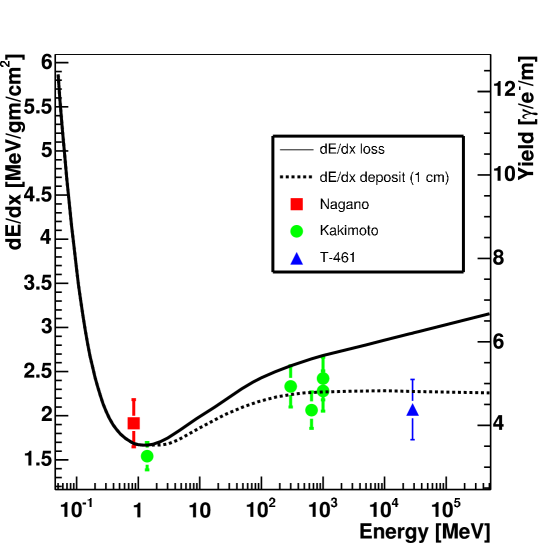
Figure 14: Comparison of the results from Nagano et al.[6], Kakimoto et al.[4], and T-461.

8 Acknowledgments

We are indebted to the SLAC accelerator operations staff for their expertise in meeting the unusual beam requirements, and to personnel of the Experimental Facilities Department for very professional assistance in preparation and installation of the equipment. We also gratefully acknowledge the many contributions from the technical staffs of our home institutions. This work was supported in part by the U.S. Department of Energy under contract number DE-AC02-76SF00515 as well as by the National Science Foundation under awards NSF PHY-0245428, NSF PHY-0305516, NSF PHY-0307098, and NSF PHY-0400053.

References

-
[1]
K. Greisen, Phys. Rev. .Lett. 16 (1966) 748;
V. A. Kuzmin, G. T. Zatsepin, Pisma Zh. Eksp. Teor. Fiz. 4 (1966) 114 [JETP Lett. 4, 78]. -
[2]
R. Abbasi et al., Phys. Rev. Lett. 92 (2004) 151101;
M. Takeda et al., Astrophys. J. 522 (1999), 225;
M. Takeda et al., Phys. Rev. Lett. 81 (1998), 1163. - [3] A. N. Bunner, Ph. D. thesis (Cornell University) (1967).
- [4] F. Kakimoto, E. C. Loh, M. Nagano, H. Okuno, M. Teshima, S. Ueno, Nucl. Instrum. Meth., A 372 (1996) 527.
- [5] M. Nagano, K. Kobayakawa, N. Sakaki, and K. Ando, Astropart. Phys. 20 (2003) 293.
- [6] M. Nagano, K. Kobayakawa, N. Sakaki, and K. Ando, Astropart. Phys. 22 (2004) 235.
-
[7]
S. Argiro, Eur. Phys. J. C 33 (2004) S947;
J. Abraham et al., Nucl. Instrum. Meth. A 523 (2004) 50;
A. Etchegoyen, Astrophys. Space Sci. 290 (2004) 379;
M. Kleifges, Nucl. Instrum. Meth. A 518 (2004) 180;
D. V. Camin, Nucl. Instrum. Meth. A 518 (2004) 172. -
[8]
M. Fukushima, Institute for Cosmic Ray Research Mid-term (2004-2009)
Maintenance Plan Proposal Book “Cosmic Ray Telescope Project”, Tokyo
University (2002);
F. Kakimoto et al., Prepared for 28th International Cosmic Ray Conferences (ICRC 2003), Tsukuba, Japan, 31 Jul - 7 Aug 2003. - [9] L. Scarsi et al., Prepared for 27th International Cosmic Ray Conferences (ICRC 2001), Hamburg, Germany, 7 Aug - 15 Aug 2001, Proceedings, 839.
-
[10]
L. Scarsi,
Prepared for 26th International Cosmic Ray Conference (ICRC 1999), Salt Lake City, Utah, 17-25 Aug 1999, Proceedings Vol. 2, 384;
J. Linsley, Prepared for 26th International Cosmic Ray Conference (ICRC 1999), Salt Lake City, Utah, 17-25 Aug 1999, Proceedings Vol. 2, 423. - [11] J. Belz et. al., “Fluorescence in Air from Showers (FLASH)”, E-165 Proposal (2002), [http://www.slac.stanford.edu/grp/rd/epac/Proposal/index.html].
- [12] J. S. T. Ng, et al., Phys. Rev. Lett. 87, 244801 (2001) [arXiv:physics/0110015].
- [13] J.A. Greenwood and H.O. Hartley, Guide to Tables in Mathematical Statistics, Princeton University Press, 1962.
- [14] L.W. Dotchin, E.L. Chupp and D.J. Pegg, Journal Chem. Phys. 59 (1973) 3960; L.L. Nicholls and W.E. Wilson, Applied Optics 7 (1968) 167.
- [15] M.A. Plum et al., Nucl. Instr.and Meth. A 492 (2002), 74.
-
[16]
S. M. Seltzer and M. J. Berger, Int. J. Appl. Radiat. Isot., 33, 1189 (1982);
R. M. Sternheimer, Berger and Seltzer, Atomic Data and Nuclear Data Tables 30, 261 (1984). - [17] R. Brun et al., GEANT3 User’s Guide, CERN DD/EE/84-1, Sept 1987, Revised Version.