Mapping dark matter with cosmic magnification

Abstract

We develop a new tool to generate statistically precise dark matter maps from the cosmic magnification of galaxies with distance estimates. We show how to overcome the intrinsic clustering problem using the slope of the luminosity function, because magnificability changes strongly over the luminosity function, while intrinsic clustering only changes weakly. This may allow precision cosmology beyond most current systematic limitations. SKA is able to reconstruct projected matter density map at smoothing scale $\sim 10^{{}^{\prime}}$ with S/N$\geq 1$, at the rate of $200$-$4000$ deg² per year, depending on the abundance and evolution of 21cm emitting galaxies. This power of mapping dark matter is comparable to, or even better than that of cosmic shear from deep optical surveys or 21cm surveys.

Introduction.— The precision mapping of the universe, and the accurate determination of cosmological parameters have been enabled by the recent generation of cosmic microwave background(CMB) experiments, galaxy and lensing surveys, and new analysis techniques. Weak gravitational lensing has emerged with a promising future of mapping dark matter directly, which would allow the inference of the state of the universe, including its dynamics and the nature of dark energy. Lensing is free from modeling assumptions, and can be accurately predicted from first principles. Several major surveys are underway, under construction or in the planning stage. Currently, most attention has focused on using the lensing induced cosmic shear[1]. But such an approach is subject to a series of difficult experimental systematics [2]. CMB lensing[3] and 21cm background lensing [4] are promising. But contaminations such as the kinetic Sunyaev Zeldovich effect [5] and/or non-Gaussianity may degrade their accuracy. In this paper we will address an alternative approach, the lensing induced cosmic magnification, which is not subject to the known problems, and could provide a robust statistical signal.

Traditionally, intrinsic clustering had presented a serious problem to measurement of cosmic magnification. The observable quantity is the surface density of galaxies above some flux threshold. A variation in this surface density is then interpreted as lensing. Unfortunately, intrinsic clustering is usually larger than the lensing induced signal. By utilizing the redshift information, intrinsic clustering can be effectively eliminated in lensing correlation functions[6, 7]. In this paper, we further show that, beyond the above statistical lensing measurement, 2D convergence $\kappa$ maps can be reconstructed with lower systematics and larger sky coverage than cosmic shear maps, by utilizing both the redshift and flux information of galaxies. 2D $\kappa$ maps not only provide independent and robust constraints on cosmology, but also are complementary to traditional shear maps. It allows one to explicitly and locally solve for non-reduced shear, an independent mode of checking E-B decomposition, and break the mass-sheet degeneracy[8].

Cosmic magnification.— Cosmic magnification causes coherent changes in the apparent galaxy number density. Let $N_{ij}$ be the observed number of galaxies (including false peaks) at the $i$-th flux bin and $j$-th redshift bin, falling into an angular pixel centered at direction $\hat{n}$ with angular size $\theta$. It can be expressed as

$$N_{ij}(\hat{n})=\bar{N}_{ij}+\bar{N}^{r}_{ij}\left[W_{ij}\kappa_{j}(\hat{n})+\delta_{g,ij}(\hat{n})\right]+\delta N_{P,ij}(\hat{n})\ .$$ (1)

The signal $W\kappa$ has unique dependence on galaxy flux through $W=2(\alpha-1)$. Here, $\alpha=-d\ln[dn/dF]/d\ln F-1$ and $dn/dF$ is the mean number of observed galaxies per flux interval $\bar{N}_{ij}=\bar{N}^{r}_{ij}+\bar{N}^{f}_{ij}$, $\bar{N}^{r}_{ij}$, $\bar{N}^{f}_{ij}$ are the mean number of detections, real galaxies and false peaks, respectively. $\delta_{g}$ and $\delta N_{P}$ are galaxy intrinsic clustering and Poisson fluctuation, respectively.

Our goal is to recover $\kappa$ of each angular pixel, given observables $N_{ij}$, $\bar{N}^{r}_{ij}$, $W_{ij}$ and $\bar{N}_{ij}$ . We consider SKA, which can detect $\sim 10^{8}$ high z galaxies through the neutral hydrogen 21cm emission line. $\kappa$ has typical value $\sim 1\%$. To beat down Poisson fluctuations, $\gtrsim 10^{4}$ galaxies per angular pixel are required. Traditionally, objects are selected at a 5$\sigma$ cut, where one can neglect the fraction of false detections. This of course also discards the majority of the signal. With a $0.5$-$\sigma$ cut, one can reduce Poisson noise at $\theta\sim 10^{{}^{\prime}}$. To increase lensing signal while reducing $\delta_{g}$ contamination, we focus on source redshifts $z\gtrsim 2$. After averaging over the full redshift range $z\geq 2$, $\delta_{g}$ is still several times larger than $\kappa$. However, $\delta N_{P}$ and $\delta_{g,ij}$ have different flux dependence to that of the signal. Weighting each galaxies by some function of their flux can suppress the prefactors of $\delta_{g}$ and $\delta N_{P}$. Intuitively, Eq. 1 implies the optimal estimator to be linear in $N_{ij}$.

The predictions rely on the assumed HI mass function $n(M_{\rm HI},z)$. We extrapolate the locally observed $n(M_{\rm HI},z)=n_{0}(z)(M_{\rm HI}/M_{*})^{-1.2}\exp(-M_{\rm HI}/M_{*})$[9] to high redshifts either assuming no evolution in both $n_{0}$ and $M_{*}$ (conservative case) or $n_{0}(z),M_{*}(z)\propto(1+z)^{1.45}\exp(-z/2.6)$ (realistic case), which is calibrated against Lyman-$\alpha$ observations (refer to [7] for details). We adopt a flat $\Lambda$CDM cosmology with $\Omega_{m}=0.3$, $\Omega_{\Lambda}=0.7$, $h=0.7$, $\sigma_{8}=0.9$, the primordial power index $n=1$, BBKS transfer function[10] and Peacock-Dodds fitting formula for the nonlinear density power spectrum [11].

The optimal estimator.— Since $z\gtrsim 2$ galaxies are mainly lensed by matter at $z\lesssim 1$, $\kappa=A-B/\chi(z)$ is an excellent approximation, where $A$ and $B$ are two constants and $\chi$ is the comoving angular diameter distance. Since $\chi(z)$ varies slowly at $z>2$, one can approximate $\kappa(\chi,\hat{n})\simeq\langle\kappa\rangle=\kappa(\langle\chi\rangle,\hat{n})$, where $\langle\chi\rangle=\sum\bar{N}^{r}_{ij}/\sum_{ij}\chi_{j}^{-1}\bar{N}^{r}_{ij}$ is the effective distance to lens . In the limit that $\bar{N}_{ij}\gg 1$, Poisson fluctuations become Gaussian. The likelihood function of $\kappa$ at an angular pixel, marginalized over $p(\delta_{g,11}\cdots\delta_{g,ij})$, the probability distribution of $\delta_{g,ij}$ of this angular pixel, is

$$L \propto \int\exp\left[-\sum_{ij}\frac{[N_{ij}-\bar{N}_{ij}-\bar{N}^{r}_{ij}(W_{ij}\kappa+\delta_{g,ij})]^{2}}{2\bar{N}_{ij}}\right]$$ (2)

$$\times p(\delta_{g,11}\cdots,\delta_{g,ij})\prod_{ij}d\delta_{g,ij}\ .$$

We choose the redshift bin size $\Delta z\gtrsim 0.2$ and angular pixel size $\sim 10^{{}^{\prime}}$ such that $\delta_{g,ij}$ of different redshift bins are uncorrelated. For this choice, the matter density dispersion of each redshift bin $\sigma_{m}\lesssim 0.1$. This verifies the neglect of high order term $\delta_{g}\kappa$ in Eq. 1 & 2.

Since $\sigma_{m}\lesssim 0.1$ and galaxy bias $b_{g}$ is unlikely bigger than several[12], it is reasonable to assume that galaxies are Gaussian distributed. Then $p(\delta_{g,11}\cdots)$ is completely determined by the covariance matrix $C_{i_{1}j_{1};i_{2}j_{2}}\equiv\langle\delta_{g,i_{1}j_{1}}(\hat{n})\delta_{g,i_{2}j_{2}}(\hat{n})\rangle$. SKA can directly and accurately measure the correlations of galaxy density fluctuations between flux bins, which are the sum of $C_{i_{1}j_{1};i_{2}j_{2}}$, correlations induced by lensing and cross terms. In the interesting range, $C_{i_{1}j_{1}i_{2}j_{2}}$ dominates. So one can take the measured sum as first guess of $C_{i_{1}j_{1};i_{2}j_{2}}$. Maximizing $L$, one obtains the optimal estimator $\hat{\kappa}$ of $\kappa$. The reconstructed $\kappa$ can in turn be applied to subtract the lensing contribution in the covariance matrix estimation. This can be done iteratively. Since the lensing contribution is small, such iteration should be stable and converge quickly.

The properties of high redshift 21cm emitting galaxies are currently poorly known. It is likely that they trace the underlying dark matter at some level, and that galaxies of different luminosities are correlated to each other. We consider this case first, and then the extreme stochastic biasing limit[13] where galaxies of different flux are uncorrelated with each other. These two cases correspond to the worst and best cases for the $\kappa$ reconstruction, respectively.

Deterministic biasing.— We first consider the case that $\delta_{g,ij}$ of different flux bins (but of the same redshift bin) are linearly correlated, namely, $\delta_{g,ij}=b_{ij}\delta_{j}$, where $\delta_{j}$ is the dark matter density of the $j$-th redshift bin. As discussed above, $b_{ij}$ can be measured iteratively. Marginalizing over $\delta_{j}$, we obtain

$$L \propto \exp\left[-\frac{(\kappa-\hat{\kappa})^{2}}{2(\Delta\kappa)^{2}}\right]\ ,$$

$$\hat{\kappa} = (\sum_{j}S_{j}-\frac{B_{j}Q_{j}}{A_{j}})(\Delta\kappa)^{2}\ ,$$

$$\Delta\kappa = \left(\sum_{j}T_{j}-\frac{Q_{j}^{2}}{A_{j}}\right)^{-1/2}$$

$$\leq \left(\bar{N}\langle W^{2}\rangle-\bar{N}\frac{\langle Wb\rangle^{2}}{\langle b^{2}\rangle}\right)^{-1/2}\ .$$

Here $A_{j}=\sum_{i}(\bar{N}^{r}_{ij}b_{ij})^{2}/\bar{N}_{ij}+1/\sigma_{j}^{2}$, $B_{j}=\sum_{i}(N_{ij}-\bar{N}_{ij})\bar{N}^{r}_{ij}b_{ij}/\bar{N}_{ij}$, $Q_{j}=\sum_{i}\bar{N}^{r,2}_{ij}W_{ij}b_{ij}/\bar{N}_{ij}$, $S_{j}=\sum_{i}(N_{ij}-\bar{N}_{ij})\bar{N}^{r}_{ij}W_{ij}/\bar{N}_{ij}$, and $T_{j}=\sum_{i}(\bar{N}^{r}_{ij}W_{ij})^{2}/\bar{N}_{ij}$. $\bar{N}$ is the mean number of galaxies in each angular pixel. $\langle\cdots\rangle$ are weighted by galaxies with the noise from false peaks taken into account.

	conservative	realistic
$n$-$\sigma$	$n_{g}$, $\langle W\rangle$,$\langle W^{2}\rangle$	$n_{g}$, $\langle W\rangle$,$\langle W^{2}\rangle$
0.5	123,-0.44,1.1	419,-0.85, 1.5
1.0	76, -0.21,1.2	290,-0.70, 1.4
2.0	40, 0.11,1.6	184,-0.49,1.4
5.0	13, 0.98,3.7	82, 0.1, 1.8
10.0	3.9, 2.0, 7.7	36, 0.73   2.9

Table 1: The predicted number of galaxies $n_{g}/1^{{}^{\prime}2}$ at $z\geq 2$, $\langle W\rangle$ and $\langle W^{2}\rangle$ for SKA deep survey with integration time $18$ days/deg².

Maximal stochasticity.— Stochasticity eases the subtraction of the intrinsic clustering signal. In this case, $\delta_{g}$ of different bins are uncorrelated. We have

$$L \propto \exp\left[-\sum_{ij}\frac{[N_{ij}-\bar{N}_{ij}-\bar{N}^{r}_{ij}W_{ij}\kappa]^{2}}{2\sigma_{ij}^{2}}\right]\ ,$$

$$\hat{\kappa} = \frac{\sum_{ij}(N_{ij}-\bar{N}_{ij})\bar{N}^{r}_{ij}W_{ij}/\sigma^{2}_{ij}}{\sum_{ij}[\bar{N}^{r}_{ij}W_{ij}]^{2}/\sigma^{2}_{ij}}\ ,$$

$$\Delta\kappa = [\partial^{2}\ln L/\partial\kappa^{2}]^{-1/2}=\left[\sum_{ij}\frac{[\bar{N}^{r}_{ij}W_{ij}]^{2}}{\sigma^{2}_{ij}}\right]^{-1/2}$$ (4)

$$\geq [\bar{N}\langle W^{2}\rangle]^{-1/2}\ \ {}^{\prime}=^{\prime}\ when\ \bar{N}^{r}_{ij}\sigma^{2}_{g,ij}\rightarrow 0\ .$$

Here, $\sigma^{2}_{ij}=\bar{N}_{ij}+\bar{N}^{r,2}_{ij}\sigma_{g,ij}^{2}$, where the first term is the shot noise and the second term is the intrinsic fluctuation of galaxy number distribution. The conditions $\bar{N}^{r}_{ij}\sigma^{2}_{g,ij}\lesssim 0.01\bar{N}_{ij}\rightarrow 0$ and $\bar{N}_{ij}\gg 1$ (for Gaussianity) can both be satisfied since galaxy bias $b_{g}$ is unlikely bigger than several[12]. A similar estimator has been derived by [14]. In two estimators, $\langle W^{2}\rangle$ and $\langle Wb\rangle$ are two key ingredients and reflect the key role of flux information.

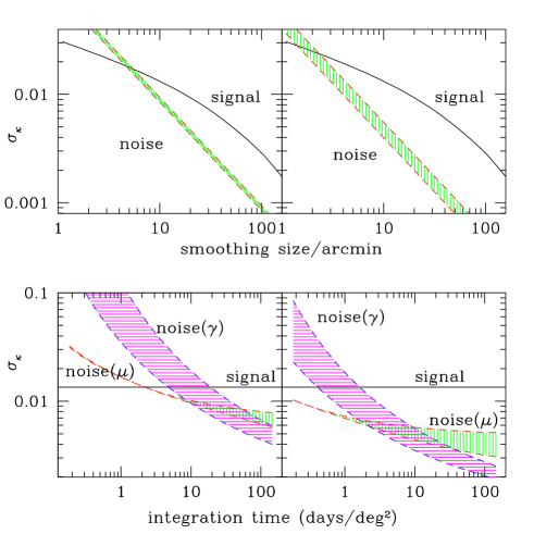
Figure 1: Estimated power of SKA to recover the lensing convergence map. Left panels and right panels correspond to the conservative case and the realistic case. We only use galaxies at $z>2$ above a $0.5$-$\sigma$ detection threshold and assume unity galaxy bias. In top panels, we fix the integration rate as 18 days/deg² and plot rms of signal (black lines) and noise (shaded regions) as function of smoothing size. Upper and lower limits of statistical errors are calculated by Eq. Mapping dark matter with cosmic magnification and Mapping dark matter with cosmic magnification, respectively. Bottom panels show the comparison between cosmic magnification ($\mu$) and cosmic shear ($\gamma$) at $10^{{}^{\prime}}$ smoothing scale. The lower and upper limit of shear measurement error are estimated using $5$-$\sigma$ and $10$-$\sigma$ cut, respectively and adopting mean ellipticity $\langle\epsilon^{2}\rangle^{1/2}=0.54$, as expected for disk galaxies. SKA is likely capable of reconstructing the $\kappa$ map with $S/N>1$ at the rate of $\sim 4000$ deg²/year. Cosmic shear quickly loses power when decreasing the integration time per deg² while cosmic magnification is less affected.

Results.— SKA is able to detect $n_{g}\gtrsim 100\ {\rm arcmin}^{-2}$ galaxies at $z\gtrsim 2$ (table I). For an integration time $t_{\rm int}=18$ days/deg², a S/N$\gtrsim 2$ can be achieved at $\theta\sim 10^{{}^{\prime}}$ (fig. 1). Deep survey configuration detects more faint galaxies, which have $W\rightarrow-2$, mimic a constant $b$ and thus do not contribute to the signal, due to the $\langle W^{2}\rangle-\langle Wb\rangle^{2}/\langle b^{2}\rangle$ facotr in Eq. 3. An optimal survey configuration should have $\langle Wb\rangle\rightarrow 0$, which can be achieved at $t_{\rm int}\sim 0.2$-$1$ day/deg² (fig. 1). Since $n_{g}$ above $0.5$-$\sigma$ decreases much more slowly than $t_{\rm int}$ (for example, for the evolution model, decreasing $t_{\rm int}$ from $180$ days/deg² to $4$ hours/deg², $n_{g}$ only decreases by a factor of $9$), it is still likely to achieve S/N$>1$ at $\theta\sim 10^{{}^{\prime}}$ and scan rate of $\sim 4000$ deg² per year (fig. 2). This will produce more lensing information ($\propto$ S/N$\times f_{\rm sky}^{1/2}$) in a one year SKA survey than SNAP will produce, which will cover $1000$ deg² sky area with S/N$\sim 2$ at smoothing scale $\theta\sim 10^{{}^{\prime}}$.

Since the SKA will have $\sim 0.3^{{}^{\prime\prime}}$ resolution at $z\sim 2$, it can resolve galaxies and measure cosmic shear. An intrinsic advantage of cosmic magnification measurement over cosmic shear measurement is that it does not require galaxies to be resolved. Thus, dwarf galaxies which are too small and too faint for reliable shear measurement still contribute to magnification measurement. Cosmic magnification exceeds cosmic shear at integration rate $\lesssim 0.2$-$10$ days/deg² (fig.1). We note that this comparison is conservative. We have neglected all systematics of shear measurement. For magnification estimation, we only select galaxies above a $0.5$-$\sigma$ detection threshold, or HI mass above ${\rm several}\times 10^{8}M_{\odot}h^{-2}$. There are numerous galaxies with HI mass $\sim 10^{7}M_{\odot}h^{-2}$[9], which can in principle be used to improve the measurement. We do not explore its potential in this paper since the luminosity function at the faint end is unclear.

Several uncertainties could degrade the signal separation. (1) The HI mass function, which is the dominant factor, as can be seen from table I and fig. 1. Here we further draw the attention on the slope of the HI mass function. For an extreme case that $\alpha\rightarrow 1$ and $W\rightarrow 0$ over a large flux range, the signal disappears. This effect can be straightforwardly estimated through the $\langle W^{2}\rangle$ and $\langle Wb\rangle$ terms in Eq. 3 & 4, once the HI mass function is measured. Since HI mass function at high $z$ is effectively unknown, we postpone the discussion in this paper. (2) The galaxy bias. For the case of deterministic biasing, if $b_{g}\propto W$, flux information is no longer useful for the separation and our method effectively fails. But since $b_{g}>0$, as long as the survey is deep enough to probe the faint end of galaxies where $W<0$, $b_{g}$ can not always mimic $W$ and the separation is always possible. (3) The galaxy distribution. When $b_{g}$ is bigger than several or smoothing size is smaller than several arc-minutes, $\delta_{g}$ is non-Gaussian. In this case, the estimators described above are no longer optimal. Optimal estimators for non-Gaussian galaxy distribution should be further investigated.

Applications.—The reconstructed $\kappa$ map can be applied to measure many lensing statistics. For this purpose, reconstructed $\kappa$ can be noisy because these statistics generally average over many angular pixels and achieve high S/N. Then the optimal estimator derived in this paper can be applied to each narrow redshift bins and allows the lensing tomography. (1)The probability density function $p(\kappa)$. $p(\kappa)$ as a function of $\kappa$ and smoothing angular size $\theta$ can provide independent constraints on cosmology. Recently [15] showed that the Wiener filter reconstruction of $p(\kappa)$ from noisy convergence map can go deep into regions where $|\kappa/\Delta\kappa|\ll 1$. We thus expect that $p(\kappa)$ can be recovered accurately from SKA. (2) Lensing power spectrum and bispectrum. The reconstructed $\kappa$ map barely has S/N$\gtrsim 5$, so it is consistent to neglect $\lesssim 10\%$ higher order terms: $O(\kappa^{2})$ terms and $\delta_{g}\kappa$ term neglected in Eq. 1 and $\kappa(\chi)-\langle\kappa\rangle$. But these terms should be taken into account for precision measurement of lensing power spectrum and bispectrum, since their statistical errors can reach $\sim 1\%$ accuracy[7]. For the linear estimator we derived, contributions of these terms to the power spectrum and bispectrum can be straightforwardly and robustly predicted. So, there is no need to derive a more complicated nonlinear estimator. (3) Cluster finding and cluster density profile. This is a promising approach to break the cluster mass sheet degeneracy. In the reconstructed maps, massive clusters at $z\sim 0.2$ show as high peaks with strength $\kappa\sim 0.1$ and size $\sim 10^{{}^{\prime}}$ and can be easily identified. These clusters are excellent objects to measure the geometry of the universe by the technique of lensing cross-correlation tomography [16]. Since S/N is so high, one can choose smoothing size $\sim 1^{{}^{\prime}}$ and measure the projected cluster density profile. Exerting a prior on cluster density profile, the reconstruction can be further improved [17]. When $\kappa\rightarrow 1$, the weak lensing condition breaks and Eq. 1 no longer holds. By utilizing the exact magnification equation, one can develop new estimator, in analogy to the reduced shear reconstruction [18]. We leave this topic for further study.

We summarize our results. Cosmic magnification is statistically more sensitive than cosmic shear because it is possible to use the large number of galaxies detected at low statistical significance. Intrinsic clustering can be subtracted because (1) magnification depends strongly on the shape of the luminosity function, which varies significantly, while intrinsic clustering depends weakly on the intrinsic luminosity itself and (2) they have different redshift dependence. Cosmic magnification shows promise as a complementary technique to map the statistically precise distribution of matter, which is not subject to most of the systematics of cosmic shear. We have worked through the specific numbers for the SKA, but the general formalism would also apply to optical spectroscopic or photometric redshift surveys.

Acknowledgments.— We thank Scott Dodelson for many helpful conversations and careful proofreading. We thank Albert Stebbins and Martin White for helpful discussions. P.J. Zhang was supported by the DOE and the NASA grant NAG 5-10842 at Fermilab.

References

- [1] A. Refregier, 2003, ARAA, 41, 645 and reference therein; M. Jarvis et al. 2003, AJ, 125, 1014; U. Pen et al. 2003, 592, 664; M. Jarvis et al. 2004, MNRAS, 352, 338; T. Chang et al. 2004, astro-ph/0408548
- [2] C. Harata et al. 2004, MNRAS, 353, 529; H. Hoekstra, 2004, MNRAS, 347, 1337; M. Jarvis et al. 2004, MNRAS, 352, 338; C. Vale et al. 2004, ApJL, 613, L1; L. van Waerbeke, et al. 2004, astro-ph/0406468; C. Heymans et al. 2005, astro-ph/0506112
- [3] U.Seljak and M. Zaldarriaga, 1999, PRL, 82, 2636; M. Zaldarriaga and U. Seljak, 1999, PRD, 5913507; W. Hu and T. Okamoto, 2002, ApJ, 574, 566; C. Hirata and U. Seljak, 2003, PRD, 68, 083002
- [4] U. Pen, 2004, New Astronomy, 9, 417; K. Sigurdson and A. Cooray, 2005, astro-ph/0502549
- [5] A. Amblard et al. 2004, New Astronomy, 9, 687
- [6] R. Scranton, et al. , 2005, astro-ph/0504510 and reference therein
- [7] P. Zhang and U. Pen, 2005, astro-ph/0504551
- [8] P. Schneider et al, 1992, Gravitational lenses, Springer-Verlag, Berlin
- [9] M. Zwaan, et al. 1997, ApJ, 490, 173
- [10] J. Bardeen et al. 1986, ApJ, 304, 15
- [11] J. Peacock and S. Dodds, 1997, MNRAS, 280, 19
- [12] H. Mo and S. White, 1996, MNRAS, 282, 347; M. Giavalisco et al. 1998, ApJ, 503, 543; V. Springel et al., 2005, Nature, 435, 629
- [13] U. Pen, 1998, ApJ, 504, 601.
- [14] B. Ménard and M. Bartelmann, 2002, A&A, 386, 784
- [15] T. Zhang and U. Pen, 2005, astro-ph/0503064
- [16] B. Jain and A. Taylor, 2003, PRL, 91, 141302; J. Zhang et al. 2003, astro-ph/0312348
- [17] S. Dodelson, 2004, PRD, 70, 023009
- [18] U. Pen, 2000, ApJ, 534, L19