Effects of clumping on temperature I: externally heated clouds

Abstract

We present a study of radiative transfer in dusty, clumpy star-forming regions. A series of self-consistent, three-dimensional, continuum radiative transfer models are constructed for a grid of models parameterized by central luminosity, filling factor, clump radius, and face-averaged optical depth. The temperature distribution within the clouds is studied as a function of this parameterization. Among our results, we find that: (a) the effective optical depth in clumpy regions is less than in equivalent homogeneous regions of the same average optical depth, leading to a deeper penetration of heating radiation in clumpy clouds, and temperatures higher by over 60 per cent; (b)penetration of radiation is driven by the fraction of open sky (FOS) – which is a measure of the fraction of solid angle along which no clumps exist; (c) FOS increases as clump radius increases and as filling factor decreases; (d) for values of FOS $>0.6-0.8$ the sky is sufficiently “open” that the temperature distribution is relatively insensitive to FOS; (e) the physical process by which radiation penetrates is preferentially through streaming of radiation between clumps as opposed to diffusion through clumps; (f) filling factor always dominates the determination of the temperature distribution for large optical depths, and for small clump radii at smaller optical depths; (g) at lower face-averaged optical depths, the temperature distribution is most sensitive to filling factors of 1 - 10 per cent, in accordance with many observations; (h) direct shadowing by clumps can be important for distances approximately one clump radius behind a clump.

1 Introduction

An understanding of the star formation process requires an understanding of the underlying density distribution in star forming regions. In a direct sense, knowledge of the density distribution can help distinguish between different potential dynamical scenarios for energy injection, collapse, fragmentation, and outflow. In a more indirect sense, the density distribution significantly affects our ability to infer source properties through its influence on thermal balance, chemistry, local emission, and the processing of radiation (radiative transfer) between the emitting region and the observer.

The density distribution is important for the dust as well as the gas. In particular, the dust forms the dominant source of opacity to visible and infrared (IR) radiation, and is the dominant source of IR continuum radiation. Perhaps more importantly, the dust dominates thermal balance by direct interaction with the radiation field (van de Hulst 1949), and through collisions with the gas (Greenberg 1971; Goldreich & Kwan 1974). As the problems of thermal balance and radiative transfer are non-local, non-linear feedback problems, comparison of detailed models with observations remain the best choice of reliably inferring the source properties.

Source geometry is a significant problem in modeling star-forming regions. While it is normal to assume some geometric symmetry, such restrictions are generally not realistic. In particular, a wealth of observations (e.g. Migenes et al. 1989; Dickman et al. 1990; Falgarone et al. 1991; Cesaroni et al. 1991; Marscher et al. 1993; Zhou et al. 1994; Plume et al. 1997; Shepherd et al. 1997) show that and fragmentation (see also Goldsmith 1996; Tauber 1996 and references therein). This is supported by dynamical models (e.g. Truelove et al. 1998; Marinho & Lepine 2000; Klapp & Sigalotti 1998; Klessen 1997) which naturally produce clumpy and fragmented structures.

Previous work on radiative transfer in dusty, clumpy environments has been undertaken (e.g. Hegmann & Kegel 2003; Witt & Gordon 1996; Varosi & Dwek 1999; Boissé 1990). However, much of the previous work has concentrated on scattering (e.g. with application to reflection nebulae), the detailed methods of solution, and/or some of the fundamental results such as ability of radiation to penetrate to apparently high optical depths. In this paper we use a 3-D monte carlo radiative transfer model to extend the previous work to a wider and different range of physical conditions. In particular, we construct a large grid of models in an effort to better delineate and understand the effects of clumpy media on radiative transfer. By controlling and varying the parameterization of the source, we attempt to disentangle some of the underlying physical causes of these effects.

In section two we describe the model. We discuss the general effects of clumping in section three. In section four, we introduce the “fraction of open sky” (FOS), and discuss the effects of number density, FOS, optical depth, filling factor, and clump size on the dust temperature distribution. We discuss the effects of shadowing in section five. Finally, we draw conclusions in section six.

2 Model

2.1 Monte carlo model and invariant parameters

We have constructed detailed, self-consistent, three-dimensional radiative transfer models through dust. The model utilizes a monte-carlo approach, combined with an approximate lambda iteration to ensure true convergence even at high optical depths. The model has been tested against existing 1-D (Egan, Leung, & Spagna 1988) and 2-D (Spagna, Leung, & Egan 1991) codes, and in modeling a 3-D source (Doty et al. 2005) with good success. Since the present study concentrates upon opaque molecular clouds where far-infrared radiaton should dominate both for external heating and emission, we ignore the effects of scattering. Test cases in both one- and multiple-dimensions show that scattering plays only a very small role on the temperature distribution within the majority of the sources.

Based upon the input parameters discussed below, we solve for the dust temperature and radiation field at each point in the model cloud. The computational volume is taken to be cubical of size 1 pc. Each model utilized an $81\times 81\times 81$ cell grid, yielding a typical resolution of $\sim 3\times 10^{16}$ cm. The region is taken to be a two-phase medium consisting of high density clumps, and a low density inter-clump medium. The clump/inter-clump density ratio is taken to be $n_{\mathrm{clump}}/n_{\mathrm{inter-clump}}=100$ from observations (e.g. Bergin et al. 1996). The external radiation field is taken from interstellar radiation field (ISRF) compiled by Mathis, Mezger, & Panagia (1983). Finally, we adopt the dust opacities in column 5 of Table 1 of Ossenkopf & Henning (1994), which have been successful at fitting observations of both high-mass (e.g., van der Tak et al. 1999, 2000) and low-mass (e.g., Evans et al. 2001) regions of star formation.

2.2 Model parameters

We adopt a uniformly distributed interclump medium interspersed with higher density clumps having $n_{\mathrm{clump}}/n_{\mathrm{inter-clump}}=100$. The clumps are randomly distributed within the computational volume. The number of clumps, and the densities of the clumps and interclump medium depend upon the filling factor ($f$), the clump radius ($r_{c}$), and the face-averaged optical depth ($\bar{\tau}$).

The filling factor specifies the fraction of the volume at high density. It is given by $f\equiv V_{\mathrm{clumps}}/V_{\mathrm{total}}$. We adopt filling factors of $f=0.01$, $0.1$, and $0.3$ in accord with observations (e.g. Snell et al. 1984; Bergin et al. 1996; Carr 1987). When all other parameters are kept fixed, a higher $f$ corresponds to a larger number of clumps, and a more nearly continuous dust distribution. Furthermore, due to optical depth constraint (see $\bar{\tau}$ below), a larger $f$ also corresponds to clumps and interclump medium of lower density.

We make the simplifying assumption that all non-overlapping clumps are spheres of radius $r_{c}$. We choose $r_{c}=0.025$ pc, $0.05$ pc, and $0.1$ pc in accord with observations (e.g. Carr 1987; Howe et al. 1993). Again, the constraint on the optical depth implies that larger clump radii yield smaller densities within the clumps.

The dust number densities are normalized by averaging the optical depth over one entire ($81\times 81$) face of the computational cube. We call this the face-averaged optical depth, and denote it by $\bar{\tau}$. This was done to simulate the optical depth / column density that might be inferred by a very large beam, although it has the same effect as normalizing to the total cloud mass. The face-averaged optical depth is taken to be $\bar{\tau}=10$, and $100$, in keeping with observations from extinction studies (Lada, Alves, & Lada 1999).

Finally, the models are specified by the strength of the internal radiation field, specified by the luminosity of the central source, $L_{*}$. We have constructed a grid having $L_{*}=0$L_⊙, $3$L_⊙, and $300$L_⊙ to represent a starless core, a low-luminosity central object, and a high-luminosity central object, respectively. However, in this paper, we restrict our report to the starless cores only ($L_{*}=0$). The others will be presented in a forthcoming paper.

The ranges of parameters specified above led to a grid of 54 models. Each model is numbered by a four-digit integer $I_{L}I_{f}I_{rc}I_{\bar{\tau}}$. The integers, and their corresponding values are given in Table 1 for reference. As an example, model 1221 has $L_{*}=0$, $f=0.01$, $r_{c}=0.025$ pc, and $\bar{\tau}=10$.

Table 1: Model input parameters

Number	$L_{*}$	$f$	$r_{c}$	$\bar{\tau}$
	(L⊙)		(pc)
1	$0$	$0.01$	$0.025$	$10$
2	$3$	$0.1$	$0.05$	$100$
3	$300$	$0.3$	$0.1$	n/a

2.3 Invariance with clump and photon randomization

One concern with “random” clump distribution and monte-carlo simulation is the reproducibility of results with different realizations of the clump distribution (i.e. different initial seeds in the clump generation), and different photon ray paths. As a test, we have considered 9 different initial seeds for the clump distributions and photon paths respectively.

To quantify the temperature distribution, we calculate a spherical average temperature, given by

$$\langle T(r)\rangle=\sum_{i}^{N}T_{i}n_{i}/\sum_{i}^{N}n_{i}.$$ (1)

Here $N$ is the number of cells a distance between $r$ and $r+\Delta r$ from the center, where $\Delta r$ is the size of a single cell, and $T_{i}$ and $n_{i}$ are the temperature and density of the cells respectively. In keeping with the viewpoint that the high density clumps mostly affect the local radiation field, while the the low density medium best probes the radiation field, the average temperature is taken only over the low-density cells.

The differences in $\langle T(r)\rangle$ between different clump distribution realizations are always much less than 1K, and are on average less than 0.1K. Based upon this (and direct comparison of later analyses) the specific realization of the density distribution does not affect our conclusions.

Figure 1: Spherical average temperature as a function of radial position for varying number of initial photons (ray pays) per cell face for the same random clumpy model.

Likewise, we have modified the number and distribution of incident photons to test for sufficient monte carlo coverage. The effect of number of photons on for $\langle T(r)\rangle$ is shown in Fig. 1. To be conservative, we adopt 100 photons per cell face, at which point differences are less than 0.05K (1 per cent).

Similarly, varying the random distribution of photon paths causes deviations of $<0.1$K, confirming that the coverage of the cells by ray-paths is sufficient to concentrate on the consequences of clumping.

3 Clumping: general

In this section we briefly discuss the general effects of clumping on the dust temperature distribution. For clarity, we directly compare a clumpy, externally heated ($L_{*}=0$), low-density ($f=0.1$), opaque ($\bar{\tau}=10$), model having small clumps ($r_{c}=0.05$ pc) to one with a uniform density distribution and the same optical depth and external heat source, so we can directly measure the effects of clumping. We have done similar comparisons for all other models, with similar results.

Figure 2: The temperature as a function of position within a clumpy (solid line) and non-clumpy (dotted line) low optical depth ($\bar{\tau}=10$) model, along the three principal axes.

Figure 3: The fractional difference in $\langle T(r)\rangle$ between a clumpy and non-clumpy externally heated ($L_{*}=0$), low optical depth ($\bar{\tau}=10$) model.

The temperature distributions along the principal axes for a representative clumpy and equivalent homogeneous model are shown in Fig. 2. To quantify the differences between the temperature distributions, in Fig. 3 we plot the fractional difference in $\langle T(r)\rangle$ between these two representative models. From these two figures, it is immediately obvious that the inclusion of clumps – even for the same $\bar{\tau}$ – changes the temperature structure significantly. In particular, the clumpy model experiences higher temperatures by up to 50 per cent toward the center, and up to $\sim 65$ per cent at intermediate radii. As a result, we conclude that clumping itself affects the temperature distribution, even when the average source mass or column density is held constant.

This result confirms the previous finding of others (e.g. Hegmann & Kegel 2003; Witt & Gordon 1996; Varosi & Dwek 1999) that the effective optical depth in a clumpy medium is less than the homogeneous value. It also suggests that it is important to understand the way in which the parameterization of the clumpy density distribution can affect the dust temperature. We address these individually below.

4 Clumping: effects of parameters

4.1 Number density

Figure 4: Distribution of temperature (solid lines, left-hand scale) and density (dotted lines, right-hand scale) for cuts along the x-, y-, and z-axes of model 1221. Other models yield qualitatively identical results.

In Fig. 4 we plot the temperature (solid lines, left hand scale) and dust number density (dotted lines, right hand scale) for cuts along the x-, y-, and z-axes. The clumps are signified by the higher density regions. As can be seen, the clumps are resolved, and appear to be of different sizes as the axes do not penetrate all clumps along a diameter. The “wiggles” and $\sim 0.1-0.2$ K deviations in the temperature distribution are not simply indicative of the uncertainties in the monte carlo calculation (see previous results, and Fig. 2). Instead, the majority are dominated by local differences in radiation field due to different amounts of blocking of radiation by the surrounding clumps (see Sect. 5 for more discussion).

As can be seen in Fig. 4, the dust temperature is lower within the high density clumps than it is within the lower-density interclump medium. Since the total emission by grains of absorption efficiency $\langle Q_{\mathrm{abs}}\pi a^{2}\rangle\propto\nu^{\beta}$ goes as $T^{4+\beta}$, one might expect a factor of 100 increase in density to lead to a decrease in temperature by a factor $100^{1/(4+\beta)}$. Given that $\beta\sim 1.8$ in the FIR for the adopted dust model, this is a decrease by a factor of $\sim 2.2$. For comparison, the average decrease within the clumps is a factor of $1.5$ with a greatest decrease a factor of $1.6$. This is due to the fact that the clump centers can be warmed by absorbing the radiation emitted from the clump edges, in effect trapping radiation within the clumps (similar to the opaque centers of centrally heated envelopes, Doty & Leung 1994).

Of even further interest is the fact that while the temperature decreases coincide with the locations of the clumps, the shape of the temperature profiles do not match the steepness of the clump/interclump interfaces. This further suggests that radiative transfer effects play a role.

4.2 Effective optical depth

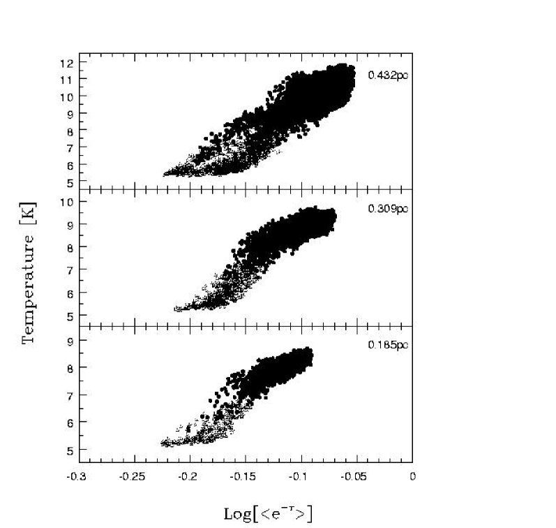
Figure 5: Temperature as a function of angle-averaged attenuation ($\langle e^{-{\tau}}\rangle$) for three distances from source center ($R_{\mathrm{out}}/3$, $R_{\mathrm{out}}/2$, and $2R_{\mathrm{out}}/3$). The solid symbols correspond to the temperature in the low density interclump medium, while the open symbols correspond to the high density clumps. This result is for model 1221. Other models are qualitatively identical.

Previous authors (e.g., Hegmann & Kegel 2003; Witt & Gordon 1996; Varosi & Dwek 1999) identified the effective optical depth ($-\ln[L_{\mathrm{AT}}/L_{*}]$), where $L_{\mathrm{AT}}$ is the attenuated flux integrated over all solid angles and $L_{*}$ is the unattenuated flux integrated over all solid angles or equivalently the average attenuation ($\langle e^{-\tau}\rangle\equiv\int e^{-\tau}d{\Omega}/\int d{\Omega}$) as a key measure of the ability of radiation to penetrate. This is reasonable, as the fewer photons penetrating leads to cooler dust, which is confirmed in Fig. 5, where we plot the dust temperature at three different positions along the x-axis as a function of $\langle e^{-\tau}\rangle$ for model 1221.

One question is left unanswered – the physical process driving the angle-averaged attenuation must be identified. There are two possibilities: (1) the ability of radiation to penetrate is dominated by general attenuation by multiple clumps along a given line of sight and attenuation by the low-density interclump medium; or (2) the radiation streams primarily through the “holes” between clumps. We consider these two possibilities in the following subsection.

4.3 Optical depth and fraction of open sky

4.3.1 Motivation and definition of $\langle\tau\rangle$ and FOS

In order to answer the question of whether and how much geometry matters in determining the local temperature/radiation field, we consider two limiting cases. These are a measure with limited geometry information, the angle-averaged optical depth ($\langle\tau\rangle$), and a measure which is dominated by geometry information, the fraction of open sky (FOS). We consider these seperately below.

If the radiation generally diffuses and is attenuated by multiple clumps or the low-density interclump medium, we might expect to find a dependence of source properties on the optical depth averaged over all directions. As a result, we define the angle-averaged optical depth to be

$$\langle\tau\rangle\equiv\int\tau(\Omega)d\Omega/\int d\Omega.$$ (2)

On the other hand, if the radiation penetrates mainly by streaming through holes between clumps, then the source properties should depend more significantly on the fraction of the sky that is uncovered by the clumps. Consequently, we also define the fraction of open sky, FOS, to be

$$\mathrm{FOS}\equiv\int qd\Omega/\int d\Omega.$$ (3)

Here $q=1$ if there is no clump along the given line of sight (i.e. if the sky is “open” in that direction), while $q=0$ if there is a clump along the given line of sight (i.e. if the sky is “closed” in that direction). Consequently, FOS=1 implies an open sky with no clumps, while FOS=0 corresponds to a closed sky where all lines of sight are blocked by clumps.

Figure 6: Distribution of temperature (solid lines, left-hand scale) and FOS (dotted lines, right-hand scale) for cuts along the x-, y-, and z-axes of model 1221. Other models yield qualitatively identical results.

As a first test of the effect of FOS on temperature, in Fig. 6 we plot the temperature (solid lines, left-hand scale) and FOS (dotted lines, right-hand scale) for cuts along the x-, y-, and z-axes, similar to Fig. 4. There is a strong correlation of dust temperature with FOS. Interestingly, the shape of the temperature distribution correlates with FOS to a much higher degree than it anti-correlates with the dust number density. This strongly suggests that FOS plays a key role, which we test in the following discussion.

4.3.2 Effect of $\langle\tau\rangle$ on temperature

Figure 7: Temperature as a function of angle-averaged optical depth ($\langle\tau\rangle$) for three distances from source center ($R_{\mathrm{out}}/3$, $R_{\mathrm{out}}/2$, and $2R_{\mathrm{out}}/3$), for a fixed FOS. This result is for model 1221. Other models are qualitatively identical.

To test the role of angle-averaged optical depth, we consider the dependence of temperature on $\langle\tau\rangle$ for a fixed FOS. In this way, we can isolate the effects of $\langle\tau\rangle$ from FOS. The FOS value here was chosen to maximize the number of data points to provide for the best possible statistics. The resulting dependence of temperature on $\langle\tau\rangle$ for three different radial positions is shown in Fig. 7. We note that the chosen FOS range is small to make the result independent of FOS, though moderate increases in the range lead to similar results.

Figure 8: Slope of the best fit temperature - $\langle\tau\rangle$ relationship divided by the uncertainty in the slope as a function of position in the source. Notice the small correlation that exists, suggesting that $\langle\tau\rangle$ is of only minimal importance in determining the temperature distribution. The dotted lines denote $\theta(\langle\tau\rangle)=\pm 3$ (i.e. a 3$\sigma$ deviation from zero). This result is for model 1221. Other models are qualitatively identical.

There appears to be little correlation of temperature with $\langle\tau\rangle$ at a given position. We quantify this by fitting the data distribution at each radial distance with a best-fit straight line. To understand the significance of the slope / correlation, we define a correlation parameter,

$$\theta({\langle\tau\rangle})\equiv m({\langle\tau\rangle})/\sigma_{m({\langle\tau\rangle})}.$$ (4)

Here, $m(\langle{\tau}\rangle)$ is the slope of the best-fit line relating the temperature and $\langle\tau\rangle$, and $\sigma_{m({\langle\tau\rangle})}$ is the uncertainty in that slope. The results are shown in Fig. 8. We have also included dashed lines at $m=\pm 3\sigma_{m({\langle\tau\rangle})}$ as a guide.

To best understand the utility of this comparison, consider a case for which the temperature and $\langle\tau\rangle$ are uncorrelated. In this case, the fit between them should yield a zero slope, and thus $\theta({\langle\tau\rangle})=0$. Likewise, a significant correlation should yield $\theta>3$ (i.e., a $3\sigma$ result). The results in Fig. 8 are much more consistent with $\theta({\langle\tau\rangle})=0$ throughout much of the cloud, and only reach $\theta({\langle\tau\rangle})=3$ for $r>0.7R_{\mathrm{out}}$. Consequently, we conclude that there may exist only a weak correlation between the dust temperature and $\langle\tau\rangle$.

4.3.3 Effect of FOS on temperature

Figure 9: Temperature as a function of fraction of open sky (FOS) for three distances from source center ($R_{\mathrm{out}}/3$, $R_{\mathrm{out}}/2$, and $2R_{\mathrm{out}}/3$), for a fixed $\langle\tau\rangle$. This result is for model 1221. Other models are qualitatively identical.

In a similar manner to $\langle\tau\rangle$, we consider the effect of FOS on temperature. In this case, we keep $\langle\tau\rangle$ fixed. In analogy with before, $\langle\tau\rangle$ was chosen to maximize the number of data points to ensure the best possible statistics. The resulting dependence of temperature on FOS for three different radial positions is shown in Fig. 9.

Figure 10: Slope of the best fit temperature - FOS relationship divided by the uncertainty in the slope as a function of position in the source. Notice the large correlation that exists, suggesting that FOS has significance in determining the temperature distribution. This result is for model 1221. Other models are qualitatively identical.

Inspection of Fig. 9 suggests that there exists some correlation of temperature with FOS. In a similar manner to $\langle\tau\rangle$, we quantify this by fitting the data distribution at each radial distance with a best-fit straight line. We again define a correlation parameter,

$$\theta({\mathrm{FOS}})\equiv m({\mathrm{FOS}})/\sigma_{m({\mathrm{FOS}})}.$$ (5)

Here, $m({\mathrm{FOS}})$ is the slope of the best-fit line relating the temperature and FOS, and $\sigma_{m({\mathrm{FOS}})}$ is the uncertainty in that slope. The results are show in Fig. 10. We have also included dashed lines at $\pm 3\sigma_{m({\mathrm{FOS}})}$ as a guide.

The results in Fig. 10 are generally not consistent with $\theta({\mathrm{FOS}})=0$, and lie at or above $\theta({\mathrm{FOS}})=3$ for a good deal of the cloud ($r>0.25R_{\mathrm{out}}$). Consequently, we can say that there exists a significant correlation between the dust temperature and FOS.

Finally, it is encouraging to note that the correlation between temperature and FOS is positive. This is expected, since a higher FOS leads to more direct heating by the external radiation field, and is evidenced by $m({\mathrm{FOS}})>0$.

4.3.4 Extension and interpretation of $\langle\tau\rangle$, FOS results

Table 2: Temperature dependence on FOS and $\langle\tau\rangle$. See text for discussion.

Model	$x_{\mathrm{max}}$	$x_{\mathrm{cut}}(\langle\tau\rangle)$	$x_{\mathrm{cut}}(\mathrm{FOS})$	$\overline{\theta(\mathrm{FOS})}/\overline{\theta(\langle\tau\rangle)}$
1111	0.00	0.64	0.77	n/a
1121	0.00	0.47	0.84	n/a
1131	0.00	0.84	0.64	n/a
1211	0.94	0.64	0.30	2.1
1221	0.55	0.69	0.27	$\infty$
1231	0.00	0.74	0.99	n/a
1311	0.99	0.10	0.30	1.4
1321	0.97	0.97	0.22	4.1
1331	0.86	0.94	0.92	n/a
1112	0.00	0.64	0.94	n/a
1122	0.00	0.49	0.94	n/a
1132	0.00	0.82	0.84	n/a
1212	0.94	0.74	0.64	1.0
1222	0.55	n/a	0.99	n/a
1232	0.00	0.79	n/a	n/a
1312	0.99	0.07	0.59	0.8
1322	0.97	0.97	0.30	1.8
1332	0.86	0.94	n/a	n/a

Figure 11: An estimate of the FOS in the outward facing hemisphere as a function of radial position. The solid lines correspond to $f=0.01$, the dotted lines to $f=0.1$, and the dashed lines to $f=0.3$. Lines without symbols correspond to $r_{c}=0.025$ pc, while those with triangles correspond to $r_{c}=0.05$ pc, and those with squares to $r_{c}=0.1$ pc. See text for details.

We can extend the discussion of FOS and $\langle\tau\rangle$ to the remainder of our family of models. The results are summarized in Table 2. In this table, we specify the fractional radial position from cloud center as $x\equiv r/R_{\mathrm{out}}$.

The results in Table 2 require an understanding of the range over which FOS or $\langle\tau\rangle$ can have a significant effect on the temperature distribution. In the table, $x_{\mathrm{max}}$ is the point beyond which, FOS does not play a significant role on the temperature distribution. We find (see Section 4.5) this occurs for $\mathrm{FOS}>0.6-0.8$.

To understand the origin and location of this region, consider a point a distance $r$ from the center of the region of radius $R_{\mathrm{out}}$. The number of clumps exterior to $r$ is $N=f(R_{\mathrm{out}}/r)^{3}(1-x)$. If these clumps are distributed about this point on the outward facing half of an equal volume sphere of radius $r_{\mathrm{eff}}=[4R_{\mathrm{out}}^{3}(1-x)/(4\pi/3)]^{1/3}$, then the fraction of open sky in the outward direction is $\mathrm{FOS}^{+}=1-Nr_{c}^{2}/2r_{\mathrm{eff}}^{2}$. We plot the resulting estimate of FOS⁺ as a function of position in Fig. 11. As can be seen, all models with a low filling factor (x1xx) have FOS${}^{+}>0.8$, as does model (x23x). For these models, FOS is not expected to play a significant role in determining the temperature distribution. As a result, the radius up to which FOS should play a role ($\equiv x_{\mathrm{max}}$) becomes zero for these models in Table 2. For other models, $0<x_{\mathrm{max}}<1$.

To understand the comparative importance of FOS vs. $\langle\tau\rangle$, we consider the average deviation of $\theta$ from zero for $x<x_{\mathrm{max}}$. This is reported in the last column of Table 2. For models in which $x_{\mathrm{max}}=0$, such an average is not possible, and the result is noted as “n/a”. For the case where only $\theta(\mathrm{FOS})>3$ for $x<x_{\mathrm{max}}$, the only meaningful correlation of temperature is with FOS, and so the result is noted as $\infty$. In all other cases, the last column is set to $\overline{\theta(\mathrm{FOS})}/\overline{\theta(\langle\tau\rangle)}$, where the bar signifies an average over all positions for which $\theta>3$ and $x<x_{\mathrm{max}}$. As can be seen by the last column of Table 2 the effect of FOS exceeds the effects of $\langle\tau\rangle$ in determining the temperature.

Finally, one may consider the size of the region over which FOS and $\langle\tau\rangle$ are important. To do this, in Table 2 we specify $x_{\mathrm{cut}}$, defined to be the position beyond which $\theta>3$. Generally $x_{\mathrm{cut}}(\langle\tau\rangle)>x_{\mathrm{cut}}(\mathrm{FOS})$. At low optical depths, this is true whenever $x_{\mathrm{max}}\neq 0$. For this set, the mean values for $x_{\mathrm{cut}}(\langle\tau\rangle)\sim 0.7$, and $x_{\mathrm{cut}}(\mathrm{FOS})\sim 0.4$. This suggests that not only is FOS (and thus photon streaming) more important than $\langle\tau\rangle$, but that it is also important deeper into the cloud than $\langle\tau\rangle$. This is not a suprise, as openings are a significantly more efficient method of carrying energy deep into the cloud. At larger optical depths, the effect is not as strong due to the fact that the less-dense interclump medium is capable of meaningful attenuation by itself.

The analysis above demonstrates that the angle-averaged optical depth does not provide sufficient information for describing a star-forming region. This is seen in the fact that the correlation of temperature with FOS is generally stronger than the correlation with $\langle\tau\rangle$, as well as the fact that the region over which FOS is important is generally larger than the region over which $\langle\tau\rangle$ is important. As a result, this suggests that indeed the ability of radiation to penetrate further into a clumpy source than a homogeneous source is due to the streaming of radiation through holes.

Figure 12: Ratio of local spherical average temperature to the value at $r=R_{\mathrm{out}}$, as a function of radial position, for a model with a clump size of $r_{c}=0.025$ pc, and $\bar{\tau}=100$. The different lines correspond to different filling factors: $f=0.01$ (solid), $f=0.1$ (dotted), and $f=0.3$ (dashed). The results are averaged over 9 different realizations of the clump distribution, and the error bars are the statistical uncertainties from the averaging.

4.4 Filling factor and clump radius

In this subsection we investigate the effects of filling factor and clump radius on the dust temperature distribution. Since $f$ and $r_{c}$ both geometrically parameterizatize the clump distribution, we account for the range of realizations in the actual clump distribution by averaging $\langle T(r)\rangle$ over nine different realizations. Finally, we note that in this subsection we present the temperature contrast ($\equiv\langle T(r_{\mathrm{in}})\rangle/T_{\mathrm{out}}$), which minimizes the effect of absolute density scaling between models.

Table 3: Temperature contrast $\langle T(r_{\mathrm{in}})\rangle/\langle T_{\mathrm{out}}\rangle$ : $\bar{\tau}=10$

$r_{c}$ (pc)	$f=0.01$	$f=0.1$	$f=0.3$
$0.025$	$0.69\pm 0.01$	$0.64\pm 0.01$	$0.56\pm 0.01$
$0.05$	$0.70\pm 0.02$	$0.67\pm 0.07$	$0.61\pm 0.07$
$0.10$	$0.70\pm 0.04$	$0.71\pm 0.07$	$0.72\pm 0.05$

4.4.1 Filling factor

Figure 12 shows a representative variation in the spherical average temperature distribution with filling factor ($f$) for $r_{c}=0.025$pc and $\bar{\tau}=100$. The temperature distributions for other models in the grid are qualitatively similar. The ratio of inner to outer temperature for the full grid (including uncertainties due to different realizations) are shown in Tables 3 and 4.

We see from these data that the role of filling factor varies with clump radius. First, the dust temperature decreases with increasing $f$ as expected, since a larger $f$ leads to a smaller FOS, and thus less heating available to the lower density medium and lower temperatures.

Second, the temperature distribution for the smallest filling factor remains essentially unchanged as the clump size changes. This is due to the high FOS throughout, so that each point is well-coupled to the external radiation field, independent of the size of the clumps.

Table 4: Temperature contrast $\langle T(r_{\mathrm{in}})\rangle/\langle T_{\mathrm{out}}\rangle$ : $\bar{\tau}=100$

$r_{c}$ (pc)	$f=0.01$	$f=0.1$	$f=0.3$
$0.025$	$0.80\pm 0.01$	$0.67\pm 0.01$	$0.58\pm 0.01$
$0.05$	$0.80\pm 0.01$	$0.69\pm 0.03$	$0.55\pm 0.02$
$0.10$	$0.81\pm 0.02$	$0.71\pm 0.03$	$0.57\pm 0.05$

Third, the effect of filling factor varies inversely with clump radius. This is expected, as FOS increases with increasing $r_{c}$, and decreasing $f$. To see this, consider the simplifying case of viewing from the center of a sphere, in which spherical clumps of radius $r_{c}$ are randomly distributed a distance $R_{\mathrm{out}}$ from the center, and in which no clumps overlap. This yields $\mathrm{FOS}=1-fR_{\mathrm{out}}/4r_{c}$. For $f=0.01-0.3$, this yields FOS $=0.63-1$ for $r_{c}=0.1$ pc, $0.25-1$ for $r_{c}=0.05$ pc, and $\sim 0-1$ for $r_{c}=0.025$ pc. In reality FOS is influenced by two further competing factors – clump overlap in projection (increases FOS), and clump distribution in distance (decreases FOS). The actual variation of FOS with model parameters is given in Fig. 13. The result roughly agrees with the estimate above. The lower trend of the actual results imply that clump overlap is not a significant effect.

These results are somewhat different for models with high optical depth, $\bar{\tau}=100$. As confirmed in Table 4, the temperature distribution at these high optical depths depends significantly on $f$, independent of $r_{c}$.

This independence of temperature on clump radius for large optical depths can can be easily understood by considering the optical depth of individual clumps for various models. For the ISRF of Mathis, Mezger, and Panagia (1983), roughly 1/2 of the total energy is contained in $\lambda<25\mu$m, 2/3 in $\lambda<115\mu$m, and 3/4 in $\lambda<360\mu$m. The optical depths of a clump at these wavelengths for $\bar{\tau}=10$ are, $1.1<\tau_{\mathrm{clump}}(25\mu\mathrm{m})<67$, $0.1<\tau_{\mathrm{clump}}(115\mu\mathrm{m})<6$, and $0.01<\tau_{\mathrm{clump}}(360\mu\mathrm{m})<0.8$. On the other hand, for $\bar{\tau}=100$ the optical depths are ten times higher, namely, $11<\tau_{\mathrm{clump}}(25\mu\mathrm{m})<670$, $1<\tau_{\mathrm{clump}}(115\mu\mathrm{m})<60$, and $0.1<\tau_{\mathrm{clump}}(360\mu\mathrm{m})<8$. This implies that the clumps for $\bar{\tau}=10$ are opaque to 1/2 of the heating radiation, but transparent to the remaining 1/2. Consequently, $f$ (and FOS) can control roughly 1/2 of the heating radiation. However, for $\bar{\tau}=100$, the clumps are opaque to 2/3 - 3/4 of the heating radiation, meaning that $f$ (and FOS) can control a greater amount of the energy that penetrates to a given depth. As a result, it is not suprising to realize that as the clumps become more opaque, filling factor and the ability of radiation to stream between the clumps becomes more important.

Figure 13: Fraction of open sky at the central point in the model cloud (FOS^c) as a function of filling factor for models $1xxx$ ($L_{*}=0$). The lines correspond to different clump radii: $r_{c}=0.025$ pc (solid), $r_{c}=0.05$ pc (dotted), and $r_{c}=0.1$ pc (dashed). Note that the results are the same for all optical depths, for a given clump distribution. Results for different realizations of clump distributions are similar.

4.4.2 Clump radius

Figure 14 shows a representative variation in the spherical average temperature distribution with clump radius ($r_{c}$) for $f=0.1$ and $\bar{\tau}=100$. Again, the temperature distributions in the other models are qualitatively similar, and the temperature contrast results are shown in Tables 3 & 4.

We see from these data that the role of clump radius varies with filling factor. In comparison to the case of filling factor, the smallest clumps yield the lowest temperatures, and the largest clumps the highest temperatures, consistent with the FOS findings in Fig. 13.

The independence of temperature with $r_{c}$ for $f=0.01$ is due to the large FOS. In particular, there exists a large number of open lines of sight to any point, making clump variation unimportant. Conversely, as $f$ increases, clump size becomes more important. This is due to the fact that high filling factor models have a commensurately greater number of small clumps. As discussed previously, many small clumps are more effective at covering the sky than fewer large clumps – see Fig. 13. Consequently, clump radius is an important factor in determining the temperature profile for high filling factors.

Figure 14: Ratio of local spherical average temperature to the value at $r=R_{\mathrm{out}}$ as a function of radial position, for a model with a filling factor of $f=0.1$ pc, and $\bar{\tau}=100$. The different lines correspond to different clump radii: $r_{c}=0.025$ (solid), $r_{c}=0.05$ (dotted), and $r_{c}=0.1$ (dashed). The results are averaged over 9 different realizations of the clump distribution, and the error bars are the statistical uncertainties from the averaging.

As before, the results differ for regions of higher optical depth, $\bar{\tau}=100$. In Table 4 we can see the variation in the temperature contrast. As discussed previously, the increasing opacity of the clumps further amplifies the effect of filling factor and FOS on the temperature distribution, leaving the effect of clump radius as unimportant.

4.4.3 Relative regions of importance

By combining the results of the two previous subsections (e.g. Fig. 13 and Tables 3 & 4), we can infer the regions of importance for filling factor and clump radius. We first consider the case of $\bar{\tau}=10$. At these moderate optical depths, we see that clump radius only becomes important for $f>0.1$. In the case of $f<0.1$, clump radius essentially plays no role and is dominated by the fact that the FOS is always high for such small filling factors.

On the other hand, we see that filling factor only becomes important for $r_{c}<0.05$ pc. For $r_{c}>0.05$ pc, the temperature is dominated by the fact that the FOS is relatively insensitive to $f$, due to the large number of holes left by scenarios with small numbers of large clumps.

Figure 15: The deviation of the temperature distribution from an equivalent homogeneous model, as specified by $\phi(f)^{2}/\phi_{\mathrm{max}}$ (see text) as a function of the filling factor, for models with $r_{c}=0.5$ pc, and $\bar{\tau}=10$.

It is interesting that the inferred values of $f$ from observations routinely fall in the range of a few per cent (e.g. Hogerheijde, Jansen, van Dishoeck 1995; Snell et al. 1984; Mundy et al. 1986; Bergin 1996). In light of the results above, this may not be a suprise. For smaller filling factors, $f$ and $r_{c}$ do not play a significant role in the temperature distribution. On the other hand, for larger filling factors, the cloud is closer to homogeneous, and more sensitive to clump radius than $f$. As a result, the temperature distribution is most sensitive to changes in $f$ for $f\sim 0.1$. While many interpretations of filling factor are not driven by continuum observations, these results are relevant since one of the dominant thermal regulators for the gas is collisions with the dust – meaning that sensitivity to $T_{\mathrm{dust}}$ near $f\sim 0.1$ can lead to sensitivity in line processes near $f\sim 0.1$.

As a test, we have run additional models $f=0.03$, and $f=0.2$ for the model numbers 1x21. In order to quantify the deviation from the homogenous model, we have calculated a parameter, $\phi^{2}\equiv\frac{1}{N}\sum(\langle T(r_{i})\rangle-\langle T_{\mathrm{hom}}(r_{i})\rangle)^{2}/\sigma(r)_{\mathrm{hom}}^{2}$. Here the sum is over radial positions, $\langle T_{hom}(r_{i})\rangle$ is the spherical average temperature for the homogenous model, and $\sigma(r)_{\mathrm{hom}}$ is the uncertainty in the temperature distribution in the homogenous model. In Fig. 15 we plot the ratio of the $\phi(f)^{2}$ to the maximum value, $\phi_{\mathrm{max}}^{2}$ as a function of filling factor. Notice that, indeed, the deviation from the homogeneous models peaks for intermediate values of $f$. In particular, the greatest sensitivity to $f$ occurs in the range $f=0.01-0.1$ – a resultin accord with the ranges of filling factors commonly reported.

When the optical depth increases to $\bar{\tau}=100$, we find that filling factor plays the dominant role over a much wider range. As a result, the sensitivity to filling factor near $f\sim 0.01-0.1$ for $\bar{\tau}=10$ is not an effect here. At high optical depth, we also find that the clump radius is not important. This is due to the fact that $f$ has a larger effect on FOS than $r_{c}$ does, and that as optical depth increases, the clumps become more opaque, thereby blocking a higher fraction of the impinging radiation.

4.5 Range of importance of FOS

From the previous discussion, FOS is necessary to describe the local radiation field and heating within a clumpy medium. Here we attempt to infer the strength of the effect of FOS on temperature. While this has been addressed in passing, here we collect and further distill that information to help draw more general conclusions.

As seen in Section 4.3.4 and Fig. 8, the greatest effect of $\theta(\mathrm{FOS})$ is at large radii. We find that this is generally true across our grid of models. As expected, these points tend to have the highest FOS. Interestingly, however, the effect of FOS is on the situations where the FOS is relatively small. This can be inferred in three ways.

First, we note that the largest values of $\theta(\mathrm{FOS})$ occur for the models that have the lowest FOS. This can be indirectly seen in that the models with the largest $\overline{\theta(\mathrm{FOS})}/\overline{\theta(\langle\tau\rangle)}$ in Table 2 tend to have the larger filling factors. As seen in Figs. 11 & 13, higher $f$ corresponds to lower values of FOS.

We can roughly quantify this by saying that FOS is important for those regions where FOS $\sim 0.5$ or so. To begin to quantify this we can consider the temperature distributions and deviations in Tables 3 & 4, together with the FOS values in Fig. 13. In particular, we note that meaningful differences in spherical average temperature occur between all models at the smallest clump radius, that essentially no variation occurs with filling factor for the largest clump radius, and that meaningful variation may occur as one changes filling factor at the intermediate clump radius. From Fig. 13 we see that the largest clump radius has values of FOS $>0.5$. On the other hand, for the smallest clump radius models, FOS varies from $\sim 0.86$ to $\sim 0.25$ as one changes $f$. Finally, for the intermediate clump radius models, as one changes from $f=0.01$ to $f=0.1$ FOS varies from $\sim 0.95$ to $\sim 0.5$, with uncertain corresponding change in the temperature distribution. But, when the difference between $f=0.01$ and $f=0.3$ is considered, there is a meaningful temperature change. Taken together, this suggests that variation in FOS for FOS $>0.5$ may not be as important as variations in FOS when FOS $<0.5$ or so.

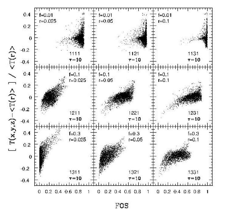
Figure 16: Deviation of temperature for a given point from the spherical average, as a function of the FOS for that point. Each tenth point is plotted. The grid of models having $\bar{\tau}$=10 (i.e. models 1xx1) are all plotted. Notice the increased spread for FOS $>0.6-0.8$, and the correlation for FOS $<0.6$ or so.

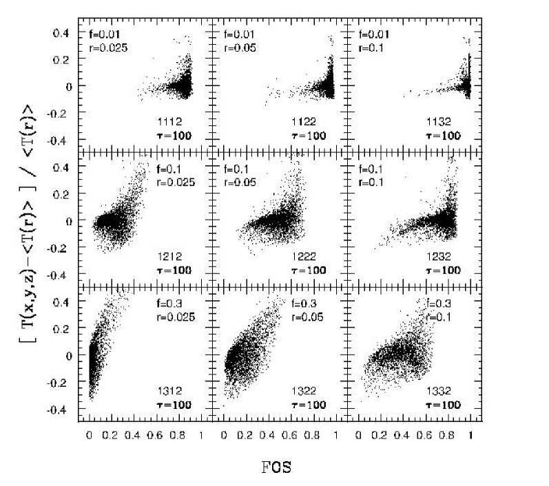
Figure 17: Deviation of temperature for a given point from the spherical average, as a function of the FOS for that point. Each tenth point is plotted. The grid of models having $\bar{\tau}$=100 (i.e. models 1xx2) are all plotted. Notice the increased spread for FOS $>0.6-0.8$, and the correlation for FOS $<0.6$ or so.

A more direct comparison suggests that FOS always plays some role, but that a change in FOS becomes increasingly important in determining the temperature for FOS $<0.6$. For FOS $>0.6-0.8$, the spread in temperatures increases. To see this in Figs. 16 & 17 we have plotted the fractional deviation of the temperature of a point from the spherical average as a function of the FOS at that point for all models in our grid. The points plotted cover all radii in the models. It is clear by inspection that FOS directly correlates with the temperature deviation. Interestingly, the correlation is strongest for FOS less than $\sim 0.6$. On the other hand, for FOS $>0.6-0.8$, there does not appear to be a direct relationship between FOS and temperature deviation. However, for the larger values of FOS the spread in temperatures is indeed greater.

Taken together, this agrees well with the idea of streaming of photons through holes in a clumpy medium. For models with a small average FOS, a position with a few extra lines of sight can receive significant additional heating. On the other hand, when the FOS for a point is high, it is well-heated by the external radiation field. However, direct shadowing of a point by a nearby clump, and attenuation by the (assumed) tenuous interclump medium can play roles. In fact, for the high optical depth models ($\bar{\tau}=100$), the ranges of temperture deviations are smaller than for low optical depth models, due to the greater attenuation by the interclump medium.

5 Shadowing

One further impact of clumps is to directly shadow points behind them, leading to lower temperatures. This effect can be seen directly in Fig. 4. In this externally heated model, points just interior to clumps are decreased in temperature relative to equivalent points not directly behind clumps. Two important questions arise: (1) over what length scale does this effect hold?, and (2) is the cause a decrease in FOS for these points?

To answer the first question, we have considered the temperature distribution as a function of distance behind clumps. The temperature at these points is consistently lower than the spherical average by $5-25$ per cent. To identify the shadowinglengthscale, we determine the distance, $d$, behind the clump at which the deviation is 1/2 the maximum. A fit of $d$ of the form $d=\delta\times r_{c}$ yields $\delta=1.2\pm 0.4$. As a result, we infer shadowing is important for lengthscale of $\sim 1.2$ clump radii behind a clump.

To answer the second question – the role of FOS – we can reconsider Fig. 6, which plots the FOS and temperature as functions of position along three axes for a representative model. Notice how well FOS correlates with temperature, especially in the shadowed regions behind clumps. This is highly suggestive that FOS is the determining factor in shadowing. More quantitatively, we can consider the fraction of sky closed (FCS) by the clump. Using the previous notation, the fraction of closed sky is $\mathrm{FCS}=r_{c}^{2}/(4d^{2})=1/4\delta^{2}$. For $\delta=1.2$, this yields $\mathrm{FCS}_{\mathrm{clump}}=0.17$, and a corresponding FOS of $0.83$. This is near the limit of FOS$=0.8$ we inferred previously above which the sky is sufficiently open for the temperature to be insensitive to FOS. As a result, we conclude that FOS (and thus actual shadowing) is the important mechanism directly behind a clump.

6 Conclusions

We have constructed a grid of three-dimensional continuum radiative transfer models for clumpy star-forming regions, in order to better delineate and understand the effects of clumping on radiative transfer. Based upon this work, we find that:

1. The inclusion of clumps – even for a constant total mass / average optical depth – can significantly change the temperature distribution within the cloud. These differences in temperature can be in excess of 60 per cent, and are due to the lower effective optical depth for clumpy media relative to equivalent homogeneous media (Sect. 3).

2. The centers of clumps are warmer than would be expected on energy density grounds due to radiation trapping (Sect. 4.1).

3. The temperature distribution is driven by the ability of radiation to penetrate, and is thus strongly correlated with the angle-averaged attenuation $\langle e^{-\tau}\rangle$ (Sect. 4.2).

4. While there exists an anti-correlation of temperature with density (Sect. 4.1), the correlation with fraction of open sky (FOS) is stronger (Sect. 4.2).

5. We find only a weak correlation of dust temperature with angle-averaged optical depth, $\langle\tau\rangle$ (Sect. 4.3.2). On the other hand, there exists a significant correlation between dust temperature and FOS (Sect. 4.3.3). This is interpreted as the dominance of streaming of radiation between clumps over diffusion through them in determining the radiation field (Sect. 4.3.4).

6. The dependence of radiation penetration on FOS versus $\langle\tau\rangle$ is robust. The stronger correlation with FOS versus $\langle\tau\rangle$ extends throughout the grid of models and for different realizations of clump distribution (Sect. 4.3.4).

7. While $\langle\tau\rangle$ may be an effect near the cloud edges, FOS is more important deeper into the cloud (Sect. 4.3.4).

8. At low face-averaged optical depths, $\bar{\tau}=10$, filling factor is more important for small clump radii than large clump radii. At large optical depths $\bar{\tau}=100$, filling factor is the dominant effect for all situations (Sect. 4.4.1).

9. The effects of clump size are only important for the largest filling factors ($f=0.3$) and lower optical depths $\bar{\tau}=10$. It is unimportant for lower filling factors or larger optical depths, $\bar{\tau}=100$ (Sect. 4.4.2).

10. For lower face-average optical depths, $\bar{\tau}=10$, filling factor is most important in determining the temperature distribution for $f=0.01-0.1$, in accordance with most observations. For very opaque clouds with $\bar{\tau}=100$, filling factor is important over a larger range (Sect. 4.4.3).

11. FOS increases as clump radius increases and as filling factor decreases (Sect. 4.4).

12. The variation of temperature with FOS is more significant in cases of small FOS (high filling factor or small clump radii), while $\langle\tau\rangle$ is relatively unimportant (Sect. 4.5).

13. For FOS $>0.6-0.8$ the sky is sufficiently open that there is little dependence of temperature on FOS (Sect. 4.5).

14. Clumps can directly shadow the regions behind them. On average, this regime extends to distance $\sim 1.2$ times the clump radius behind the clump, where the clump only subtends a small fraction of the sky (Sect. 5).

References

- [1996] Bergin, E. A., Snell, R. L., & Goldsmith, P. F. 1996, ApJ, 460, 343
- [1990] Boisse, P. 1990, A&A, 228, 483
- [1987] Carr, J. S. 1987, ApJ, 323, 170
- [1991] Cesaroni, R., Walmsley, C. M., Koempe, C., & Churchwell, E. 1991, A&A, 252, 278
- [1990] Dickman, R. L., Horvath, M. A., & Margulis, M. 1990, ApJ, 365, 586
- [2005] Doty, S. D., Everett, S. E., Shirley, Y. L., Evans, N. J., & Palotti, M. L. 2005, MNRAS, 359, 228
- [1994] Doty, S. D., & Leung, C. M. 1994, ApJ, 424, 729
- [1988] Egan, M. P., Leung, C. M., & Spagna, G. F., Jr. 1988, Comput. Phys. Comm., 48, 271
- [2001] Evans II, N. J., Rawlings, J. M. C., Shirley, Y. L., & Mundy, L. G. 2001, ApJ, 557, 193
- [1991] Falgarone, E., Phillips, T. G., & Walker, C. K. 1991, ApJ, 378, 186
- [1974] Goldreich, P., & Kwan, J. 1974, ApJ, 189, 441
- [1996] Goldsmith, P. F. 1996, in Amazing Light, R. Y. Chiao, ed., Springer Verlag, New York, p. 285
- [1971] Greenberg, J. M. 1971, A&A, 12, 240
- [2003] Hegmann, M., & Kegel, W. H. 2003, MNRAS, 342, 453
- [1995] Hogerheijde, M. R., Jansen, D. J., & van Dishoeck, E. F. 1995, A&A, 294, 792
- [1993] Howe, J. E., Jaffe, D. T., Grossman, E. N., Wall, W. F., Mangum, J. G., & Stacey, G. J. 1993, ApJ, 410, 179
- [1998] Klapp, J., & Sigalotti, L. D. G. 1998, ApJ, 504, 158
- [1997] Klessen, R. 1997, MNRAS, 292, 11
- [1999] Lada, C. J., Alves, J., & Lada, E. A. 1999, ApJ, 512, 250
- [2000] Marinho, E. P., & Lepine, J. R. D. 2000, A&AS, 142, 165
- [1993] Marscher, A. P., Moore, E. M., & Bania, T. M. 1993, ApJ, 419, 101L
- [1983] Mathis, J. S., Mezger, P. G., & Panagia, N. 1983, A&A, 128, 212
- [1989] Migenes, V., Johnston, K. J., Pauls, T. A., & Wilson, T. L. 1989, ApJ, 347, 294
- [1986] Mundy, L. G., Evans, N. J. II, Snell, R. L., Goldsmith, P. F., & Bally, J. 1986, ApJ, 306, 670
- [1994] Ossenkopf, V., & Henning, Th. 1994, A&A, 291, 943
- [1997] Plume, R., Jaffe, D. T., Evans, N. J. II, Martin-Pintado, J., & Gomez-Gonzalez, J. 1997, ApJ, 476, 730
- [1997] Shepherd, D. S., Churchwell, E., & Wilner, D. J. 1997, ApJ, 482, 355
- [1984] Snell, R. L., Goldsmith, P. F., Erickson, N. R., Mundy, L. G., & Evans, N. J. II 1984, ApJ, 276, 625
- [1991] Spagna, G. F. Jr., Leung, C. M., & Egan, M. P. 1991, ApJ, 379, 232
- [1996] Tauber, J. A. 1996, A&A, 315, 591
- [1998] Truelove, J. K., Klein, R. I., McKee, C. F., et al. 1998, ApJ, 495, 821
- [1949] van de Hulst, H. C. 1949, Rech. astr. Obs., Utrecht, 11, Part 2
- [1999] van der Tak, F. F. S., et al. 1999, ApJ, 522, 991
- [2000] van der Tak, F. F. S., et al. 2000, ApJ, 537, 283
- [1999] Varosi, F., & Dwek, E. 1999, ApJ, 523, 265
- [1996] Witt, A. N., & Gordon, K. D. 1996, ApJ, 463, 681
- [1994] Zhou, S., Evans, N. J. II, Wang, Y., Peng, R., & Lo, K. Y. 1994, ApJ, 433, 131