Particle Acceleration and the Production of Relativistic Outflows in Advection-Dominated Accretion Disks with Shocks

Abstract

Relativistic outflows (jets) of matter are commonly observed from systems containing black holes. The strongest outflows occur in the radio-loud systems, in which the accretion disk is likely to have an advection-dominated structure. In these systems, it is clear that the binding energy of the accreting gas is emitted primarily in the form of particles rather than radiation. However, no comprehensive model for the disk structure and the associated outflows has yet been produced. In particular, none of the existing models establishes a direct physical connection between the presence of the outflows and the action of a microphysical acceleration mechanism operating in the disk. In this paper we explore the possibility that the relativistic protons powering the jet are accelerated at a standing, centrifugally-supported shock in the underlying accretion disk via the first-order Fermi mechanism. The theoretical analysis employed here parallels the early studies of cosmic-ray acceleration in supernova shock waves, and the particle acceleration and disk structure are treated in a coupled, self-consistent manner based on a rigorous mathematical approach. We find that first-order Fermi acceleration at standing shocks in advection-dominated disks proves to be a very efficient means for accelerating the jet particles. Using physical parameters appropriate for M87 and Sgr A${}^{*}\,$, we verify that the jet kinetic luminosities computed using our model agree with estimates based on observations of the sources.

1 INTRODUCTION

A large body of observational evidence has established that extragalactic relativistic jets are commonly associated with radio-loud active galactic nuclei (AGNs), which may contain hot, advection-dominated accretion disks. However, the precise nature of the mechanism responsible for transferring the gravitational potential energy from the infalling matter to the small population of nonthermal particles that escape to form the jet is not yet clear (see, e.g., Livio 1999). The most promising jet acceleration scenarios proposed so far are the Blandford-Znajek mechanism (Blandford & Znajek 1977) and the electromagnetic cocoon model (Lovelace 1976; Blandford & Payne 1982), both of which involve the extraction of energy from the rotation of the black hole in order to power the outflow. While conceptually attractive, one finds that the complex physics involved in these models tends to obscure the nature of the fundamental microphysical processes. In particular, the introduction of the relativistic particles that escape to form the jet is usually made in an ad hoc manner without any reference to the dynamics of the associated accretion disk, although recent magnetohydrodynamical simulations carried out by De Villiers et al. (2005) and McKinney & Gammie (2004) have achieved a higher level of self-consistency. Given the relative complexity of the electromagnetic models, it is natural to ask whether the outflows can be explained in terms of well-understood microphysical processes operating in the hot, tenuous disk, such as the possible acceleration of the jet particles at a standing accretion shock.

It has been known for some time that inviscid accretion disks can display both shocked and shock-free (i.e., smooth) solutions depending on the values of the energy and angular momentum per unit mass in the gas supplied at a large radius (e.g., Chakrabarti 1989a; Chakrabarti & Molteni 1993; Kafatos & Yang 1994; Lu & Yuan 1997; Das, Chattopadhyay, & Chakrabarti 2001). Shocks can also exist in viscous disks if the viscosity is relatively low (Chakrabarti 1996; Lu, Gu, & Yuan 1999), although smooth solutions are always possible for the same set of upstream parameters (Narayan, Kato, & Honma 1997; Chen, Abramowicz, & Lasota 1997). Hawley, Smarr, & Wilson (1984a, 1984b) have shown through general relativistic simulations that if the gas is falling with some rotation, then the centrifugal force can act as a “wall,” triggering the formation of a shock. Furthermore, the possibility that shock instabilities may generate the quasi-periodic oscillations (QPOs) observed in some sources containing black holes has been pointed out by Chakrabarti, Acharyya, & Molteni (2004), Lanzafame, Molteni, & Chakrabarti (1998), Molteni, Sponholz, & Chakrabarti (1996), and Chakrabarti & Molteni (1995). Nevertheless, shocks are “optional” even when they are allowed, and one is always free to construct models that avoid them. However, in general the shock solution possesses a higher entropy content than the shock-free solution, and therefore we argue based on the second law of thermodynamics that when possible, the shocked solution represents the preferred mode of accretion (Becker & Kazanas 2001; Chakrabarti & Molteni 1993).

Our primary objective in this paper is to explore the consequences of the presence of a shock in an ADAF disk for the acceleration of the nonthermal particles in the observed jets. The question of whether or not viscosity needs to be included in the disk model is difficult to answer in general. Several authors have shown that shock solutions are possible in viscous (e.g., Chakrabarti 1990, 1996; Lu, Gu, & Yuan 1999; Chakrabarti & Das 2004) as well as inviscid disks (e.g., Chakrabarti 1989a, 1989b; Abramowicz & Chakrabarti 1990; Yang & Kafatos 1995; Chakrabarti 1996; Das, Chattopadhyay, & Chakrabarti 2001). In particular, Chakrabarti (1990) and Chakrabarti & Das (2004) demonstrated that shocks can exist in viscous disks if the angular momentum and the viscosity are relatively low. Since the acceleration of particles in shocked disks has never been investigated before, in this first study we shall focus on inviscid flows containing isothermal shocks (e.g., Chakrabarti 1989a; Kafatos & Yang 1994; Lu & Yuan 1997), while deferring the treatment of viscous disks to future work. However, it is clearly important to address the potential connection between this idealized, inviscid calculation and the physical properties of real accretion disks, which undoubtedly have nonzero viscosity. We argue that the results presented here should be qualitatively similar to those obtained in a viscous disk provided a shock is present, in which case efficient first-order Fermi acceleration is expected to occur. While the possible existence of standing shocks in viscous disks is a controversial issue at the present time, we believe that the work of Chakrabarti (1990, 1996), Lu, Gu, & Yuan (1999), and Chakrabarti & Das (2004) provides sufficient support for the possibility to motivate the present investigation.

Although the effect of a standing shock in heating the gas in the post-shock region has been examined by a number of previous authors for both viscid (Chakrabarti & Das 2004; Lu, Gu, & Yuan 1999; Chakrabarti 1990) and inviscid (e.g., Lu & Yuan 1997, 1998; Yang & Kafatos 1995; Abramowicz & Chakrabarti 1990) disks, the implications of the shock for the acceleration of nonthermal particles in the disk have not been considered in detail before. However, a great deal of attention has been focused on particle acceleration in the vicinity of supernova-driven shock waves as a possible explanation for the observed cosmic-ray energy spectrum (Blandford & Ostriker 1978; Jones & Ellison 1991). In the present paper we consider the analogous process occurring in hot, advection-dominated accretion flows (ADAFs) around black holes. These disks are ideal sites for first-order Fermi acceleration at shocks because the plasma is collisionless and therefore a small fraction of the particles can gain a great deal of energy by repeatedly crossing the shock. Shock acceleration in the disk therefore provides an intriguing possible explanation for the powerful outflows of relativistic particles observed in many radio-loud systems (Le & Becker 2004).

The dynamical model for the disk/shock/outflow employed here was discussed by Le & Becker (2004), who demonstrated that the predicted kinetic power in the jets agrees with the observational estimates for M87 and Sgr A${}^{*}\,$. Here we present a more detailed development of the dynamical model, including a careful examination of the implications of the shock acceleration process for the evolution of the relativistic particle distribution in the disk and the jet. The number and energy densities of the relativistic particles are determined along with the hydrodynamical structure of the disk in a self-consistent manner by solving the fluid dynamical conservation equations and the transport equation simultaneously using a rigorous mathematical approach. In this sense, the model presented here represents a new type of synthesis between studies of accretion dynamics and particle transport.

The remainder of the paper is organized as follows. In § 2 we discuss the ADAF model assumptions and the possibility of shock acceleration in ADAF disks, and the general structure of the disk/shock model is examined in § 3. The isothermal shock jump conditions and the asymptotic variations of the physical parameters at both large and small radii are discussed in § 4. In § 5 we analyze the steady-state transport equation governing the distribution of the relativistic particles in the disk and the jet. Solutions for the number and energy density distributions of the relativistic particles are obtained in § 6, and detailed applications to the disks/outflows in M87 and Sgr A${}^{*}\,$are presented in § 7. The astrophysical implications of our results are discussed in § 8.

2 MODEL BACKGROUND

Accretion onto a black hole involves differentially-rotating flows in which the viscosity plays an essential role in transporting angular momentum outward, thereby allowing the accreting gas to spiral in toward the central mass (Pringle 1981). In the ADAF model, it is assumed that the mass accretion rate is much smaller than the Eddington rate,

$$\dot{M}_{\rm E}\equiv c^{-2}\,\beta^{-1}\,L_{\rm E}=2.2\times 10^{-9}\,\beta^{-1}\left({M\over M_{\odot}}\right)\ \ {\rm M_{\odot}\ yr^{-1}}\ ,$$ (1)

where the efficiency parameter $\beta$ is of order $\sim 10\%$, and the Eddington luminosity is defined by $L_{\rm E}\equiv 4\pi\,GMm_{p}\,c/\sigma_{{}_{\rm T}}$ for pure, fully-ionized hydrogen, with $\sigma_{{}_{\rm T}}$, $M$, $m_{p}$, and $c$ denoting the Thomson cross section, the black-hole mass, the proton mass, and the speed of light, respectively. Due to the sub-Eddington accretion rates in these systems, the plasma is rather tenuous, and this strongly inhibits the efficiency of two-body radiative processes such as free-free emission. The gas is therefore unable to cool effectively within an accretion time, and consequently the gravitational potential energy dissipated by viscosity is stored in the gas as thermal energy instead of being radiated away (e.g., Narayan, Kato, & Honma 1997). The low density also reduces the level of Coulomb coupling between the ions and the electrons, resulting in a two-temperature configuration with the ion temperature ($T_{i}\sim 10^{12}\rm K$) close to the virial value, and a much lower electron temperature ($T_{e}\sim 10^{9}\rm K$). In this scenario, most of the energy is advected across the horizon into the black hole, and the resulting X-ray luminosity is far below the Eddington value (Becker & Le 2003; Becker & Subramanian 2005).

When the ion temperature is close to the virial temperature, as in ADAFs, the disk is gravitationally unbound (e.g., Narayan, Kato, & Honma 1997; Blandford & Begelman 1999; Becker, Subramanian, & Kazanas 2001). It follows that the original ADAF model was not entirely self-consistent since it neglected outflows. This motivated Blandford & Begelman (1999) to propose the self-similar advection-dominated inflow-outflow solution (ADIOS) to address the question of self-consistency by including the possibility of powerful winds that carry away mass, energy, and angular momentum. In this Newtonian, nonrelativistic model, the dynamical solutions are not applicable near the event horizon, and therefore the ADIOS approach cannot be used to obtain a global understanding of the disk structure. This led Becker, Subramanian, & Kazanas (2001) to modify the ADIOS scenario to include general relativistic effects by replacing the Newtonian potential with the pseudo-Newtonian form (Paczyński & Wiita 1980)

$$\Phi(r)\equiv{-GM\over r-r_{{}_{\rm S}}}\ ,$$ (2)

where $r_{{}_{\rm S}}=2GM/c^{2}$ is the Schwarzschild radius for a black hole of mass $M$. This modified model is known as the self-similar relativistic advection-dominated inflow-outflow solution (RADIOS). Despite the success of the self-similar RADIOS model in describing the general features of the disk/outflow structure, it does not provide a comprehensive picture since no explicit microphysical acceleration mechanism is included. It is therefore natural to explore possible extensions to the ADAF scenario that incorporate a concrete acceleration mechanism capable of powering the outflows.

The idea of shock acceleration in the environment of AGNs was first suggested by Blandford & Ostriker (1978). Subsequently, Protheroe & Kazanas (1983) and Kazanas & Ellison (1986) investigated shocks in spherically-symmetric accretion flows as a possible explanation for the energetic radiation emitted by many AGNs. However, in these papers the acceleration of the particles was studied without the benefit of a detailed transport equation, and the assumption of spherical symmetry precludes the treatment of acceleration in disks. The state of the theory was advanced by Webb & Bogdan (1987) and Spruit (1987), who employed a transport equation to solve for the distribution of energetic particles in a spherical accretion flow characterized by a self-similar velocity profile terminating at a standing shock. While more quantitative in nature than the earlier models, these solutions are not applicable to disks since the geometry is spherical and the velocity distribution is inappropriate. Hence none of these previous models can be used to develop a single, global, self-consistent picture for the acceleration of relativistic particles in an accretion disk containing a shock.

The success of the diffusive (first-order Fermi) shock acceleration model in the cosmic-ray context suggests that the same mechanism may be responsible for powering the outflows commonly observed in radio-loud systems containing black holes. As a preliminary step in evaluating the potential relevance of shock acceleration as a possible explanation for the observed outflows, we need to consider the basic physical properties of the hot plasma in ADAF disks. One of the critical issues for determining the efficiency of shock acceleration in accretion disks is the role of particle-particle collisions in thermalizing the high-energy ions. The mean free path for ion-ion collisions is given in cgs units by (Subramanian, Becker, & Kafatos 1996)

$$\lambda_{ii}=1.8\times 10^{5}\,{T_{i}^{2}\over N_{i}\ln\Lambda}\ ,$$ (3)

where $N_{i}$ and $T_{i}$ denote the thermal ion number density and temperature, respectively, and $\ln\Lambda$ is the Coulomb logarithm. In ADAF disks, $\lambda_{ii}$ greatly exceeds the vertical thickness of the disk, and therefore the shock and the flow in general are collisionless. However, the mean free path $\lambda_{\rm mag}$ for collisions between ions and magnetohydrodynamical (MHD) waves is much shorter than $\lambda_{ii}$ for the thermal particles, and it is much longer than $\lambda_{ii}$ for the relativistic particles (Ellison & Eichler 1984; Subramanian, Becker, & Kafatos 1996). The increase in $\lambda_{\rm mag}$ with increasing particle energy reflects the fact that the high-energy particles will interact only with the highest-energy MHD waves. The low-energy background particles therefore tend to thermalize the energy they gain in crossing the shock due to collisions with magnetic waves. Conversely, the relativistic particles are able to diffuse back and forth across the shock many times, gaining a great deal of energy while avoiding thermalization due to the longer mean free path.

The probability of multiple shock crossings decreases exponentially with the number of crossings, and the mean energy of the particles increases exponentially with the number of crossings. This combination of factors naturally gives rise to a power-law energy distribution, which is a general characteristic of Fermi processes (Fermi 1954). Two effects limit the maximum energy that can be achieved by the particles. First, at very high energies the particles will tend to lose energy to the waves due to recoil. Second, the mean free path $\lambda_{\rm mag}$ will eventually exceed the thickness of the disk as the particle energy is increased, resulting in escape from the disk without further acceleration.

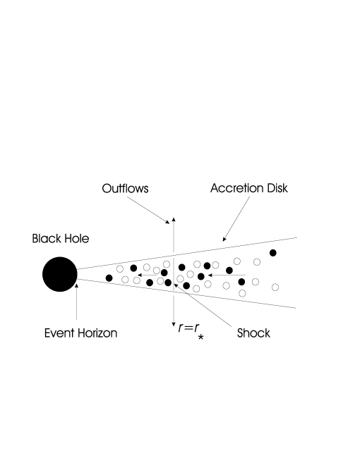
Figure 1: Schematic representation of our disk/shock/outflow model. The filled circles in the disk represent the test particles, and the unfilled circles represent the background gas. The test particles are injected at the shock location.

3 TRANSONIC FLOW STRUCTURE

As discussed in § 1, various authors have established that shocks can exist in both viscid and inviscid disks. In this first study of particle acceleration in shocked disks, we shall focus on the inviscid case because it is the most straightforward to analyze from a mathematical viewpoint, and also because it serves to illustrate the basic physical principles involved. Moreover, we expect that the results obtained in the viscous case will be qualitatively similar to those presented here since efficient Fermi acceleration will occur whether or not viscosity is present, provided the flow contains a shock. The equations governing the disk structure can yield solutions that include three possible types of standing shocks, namely (i) Rankine-Hugoniot shocks, where the effective cooling processes are so inefficient that no energy is lost from the surface of the disk, (ii) isentropic shocks, where the entropy generated at the shock is comparable to the amount radiated away, and (iii) isothermal shocks, where the cooling processes are so efficient that the post-shock sound speed and disk thickness remain the same as the pre-shock values. In the isothermal case, the shock must radiate away both energy and entropy through the upper and lower surfaces of the disk (e.g., Chakrabarti 1989a, 1989b; Abramowitz $\&$ Chakrabarti 1990). This renders the isothermal shock model particularly useful from the point of view of modeling outflows, since the energy lost from the shock can be identified with that powering the jet. On the other hand, Rankine-Hugoniot shocks cannot be used if we are interested in any kind of escape. The isentropic shock is an intermediate case. In this paper, we shall focus exclusively on the isothermal shock model since this case provides the strongest potential connection with the observed outflows.

The model considered here is depicted schematically in Figure 1. In this scenario, the gas is accelerated gravitationally toward the central mass, and experiences a shock transition due to an obstruction near the event horizon. The obstruction is provided by the “centrifugal barrier,” which is located between the inner and outer sonic points. Particles from the high-energy tail of the background Maxwellian distribution are accelerated at the shock discontinuity via the first-order Fermi mechanism, resulting in the formation of a nonthermal, relativistic particle distribution in the disk. The spatial transport of the energetic particles within the disk is a stochastic process based on a three-dimensional random walk through the accreting background gas. Consequently, some of the accelerated particles diffuse to the disk surface and become unbound, escaping through the upper and lower edges of the cylindrical shock to form the outflow, while others diffuse outward radially through the disk or advect across the event horizon into the black hole.

In order to analyze the connection between the disk/shock model and the transport/acceleration of the relativistic particles, we consider the set of physical conservation equations employed by Chakrabarti (1989a) and Abramowicz & Chakrabarti (1990), who investigated the structure of a one-dimensional, steady-state, axisymmetric, inviscid accretion flow based on the vertically-averaged conservation equations. The effects of general relativity are incorporated in an approximate manner by utilizing the pseudo-Newtonian form for the gravitational potential per unit mass given by equation (2). The use of such a potential allows one to investigate the complicated physical processes taking place in the accretion disk within the context of a semi-classical framework while maintaining good agreement with fully relativistic calculations (see, e.g., Narayan, Kato, & Honma 1997; Becker & Subramanian 2005). The pseudo-Newtonian potential correctly reproduces the radius of the event horizon, the marginally bound orbit, and the marginally stable orbit (Paczyński $\&$ Wiita 1980). Furthermore, the dynamics of freely-falling particles near the event horizon computed using this potential agree perfectly with the results obtained using the Schwarzschild metric, although time dilation is not included (Becker & Le 2003).

3.1 Transport Rates

Becker & Le (2003) and Becker & Subramanian (2005) demonstrated that three integrals of the flow are conserved in viscous ADAF disks, namely, the mass transport rate

$$\dot{M}=4\pi rH\rho\,v\ ,$$ (4)

the angular momentum transport rate

$$\dot{J}=\dot{M}r^{2}\,\Omega-\mathcal{G}\ ,$$ (5)

and the energy transport rate

$$\dot{E}=-\mathcal{G}\,\Omega+\dot{M}\left({1\over 2}\,v_{\phi}^{2}+{1\over 2}\,v^{2}+{P+U\over\rho}+\Phi\right)\ ,$$ (6)

where $\rho$ is the mass density, $v$ is the radial velocity (defined to be positive for inflow), $\Omega$ is the angular velocity, ${\cal G}$ is the torque, $H$ is the disk half-thickness, $v_{\phi}=r\,\Omega$ is the azimuthal velocity, $U$ is the internal energy density, and $P=(\gamma-1)U$ is the pressure. Each of the various quantities represents a vertical average over the disk structure. We also assume that the ratio of specific heats, $\gamma$, maintains a constant value throughout the flow. Note that all of the transport rates $\dot{M}$, $\dot{J}$, and $\dot{E}$ are defined to be positive for inflow.

The torque ${\cal G}$ is related to the gradient of the angular velocity $\Omega$ via the usual expression (e.g., Frank et al. 2002)

$$\mathcal{G}=-4\pi r^{3}H\rho\,\nu{d\Omega\over dr}\ ,$$ (7)

where $\nu$ is the kinematic viscosity. The disk half-thickness $H$ is given by the standard hydrostatic prescription

$$H(r)={a\over\Omega_{\rm K}}\ ,$$ (8)

where $a$ represents the adiabatic sound speed, defined by

$$a(r)\equiv\left({\gamma P\over\rho}\right)^{1/2}\ ,$$ (9)

and $\Omega_{\rm K}$ denotes the Keplerian angular velocity of matter in a circular orbit at radius $r$ in the pseudo-Newtonian potential (eq. [2]), defined by

$$\Omega_{\rm K}^{2}\equiv{GM\over r(r-r_{{}_{\rm S}})^{2}}={1\over r}{d\Phi\over dr}\ .$$ (10)

The quantities $\dot{M}$ and $\dot{J}$ are constant throughout the flow, and therefore they represent the rates at which mass and angular momentum, respectively, enter the black hole. The energy transport rate $\dot{E}$ generally remains constant, although it will jump at the location of an isothermal shock if one is present in the disk. We can eliminate the torque ${\cal G}$ between equations (5) and (6) and combine the result with equation (9) to express the energy transport per unit mass as

$$\epsilon\equiv{\dot{E}\over\dot{M}}={1\over 2}\,v^{2}-{1\over 2}\,{\ell^{2}\over r^{2}}+{\ell_{0}\ell\over r^{2}}+{a^{2}\over\gamma-1}+\Phi\ ,$$ (11)

where $\ell(r)\equiv r^{2}\,\Omega(r)$ and $\ell_{0}\equiv\dot{J}/\dot{M}$ denote the specific angular momentum at radius $r$ and the (constant) angular momentum transport per unit mass, respectively. Note that equation (11) is valid for both viscid and inviscid flows.

3.2 Inviscid Flow Equations

In the present application, viscosity is neglected, and therefore ${\cal G}=0$ and the specific angular momentum is given by

$$\ell(r)=\ell_{0}={\rm constant}$$ (12)

throughout the disk. It follows that the flow is purely adiabatic, except at the location of a possible isothermal shock (Becker & Le 2003). In the inviscid case, equation (11) reduces to

$$\epsilon={1\over 2}\,v^{2}+{1\over 2}\,{\ell^{2}\over r^{2}}+{a^{2}\over\gamma-1}+\Phi\ .$$ (13)

The resulting disk/shock model depends on three free parameters, namely the energy transport per unit mass $\epsilon$, the specific heats ratio $\gamma$, and the specific angular momentum $\ell$. The value of $\epsilon$ will jump at the location of an isothermal shock if one exists in the disk, but the value of $\ell$ remains constant throughout the flow. This implies that the specific angular momentum of the particles escaping through the upper and lower surfaces of the cylindrical shock must be equal to the average value of the specific angular momentum for the particles remaining in the disk, and therefore the outflow exerts no torque on the disk (Becker, Subramanian, & Kazanas 2001). Since the flow is purely adiabatic in the absence of viscosity, the pressure and density variations are coupled according to

$$P=D_{0}\,\rho^{\gamma}\ ,$$ (14)

where $D_{0}$ is a parameter related to the specific entropy that remains constant except at the location of the isothermal shock if one is present.

By combining equations (4), (8), (9), (10), and (14), we find that the quantity

$$K\equiv r^{3/2}\,(r-r_{{}_{\rm S}})\,v\,a^{(\gamma+1)/(\gamma-1)}$$ (15)

is conserved throughout an adiabatic disk, except at the location of an isothermal shock. Following Becker & Le (2003), we refer to $K$ as the “entropy parameter,” and we note that the entropy per particle $S$ is related to $K$ via

$$S=k\ln K+c_{0}\ ,$$ (16)

where $k$ is the Boltzmann constant and $c_{0}$ is a constant that depends on the composition of the gas but is independent of its state.

3.3 Critical Conditions

By combining equations (13) and (15), one can solve for the flow velocity $v$ as a function of $r$ using a simple root-finding procedure. However, in order to understand the implications of the transonic (critical) nature of the accretion flow, we must also analyze the properties of the “wind equation,” which is the first-order differential equation governing the flow velocity $v$. By differentiating equation (13) with respect to $r$, we obtain the steady-state radial momentum equation

$$v{dv\over dr}={\ell^{2}\over r^{3}}-{d\Phi\over dr}-\left({2\,a\over\gamma-1}\right){da\over dr}\ .$$ (17)

The derivative of the sound speed appearing on the right-hand side of this expression can be evaluated by using equations (10) and (15) to write

$${1\over a}{da\over dr}=\left({\gamma-1\over\gamma+1}\right)\left[{1\over\Omega_{\rm K}}{d\Omega_{\rm K}\over dr}-{1\over v}{dv\over dr}-{1\over r}\right]\ .$$ (18)

We can now construct the wind equation by combining equations (10), (17), and (18), which yields

$${1\over v}{dv\over dr}={N\over D}\ ,$$ (19)

where the numerator and denominator functions $N$ and $D$ are given by

$$N={GM\over(r-r_{{}_{\rm S}})^{2}}-{\ell^{2}\over r^{3}}+{a^{2}\over\gamma+1}\left[{3r_{{}_{\rm S}}-5r\over r(r-r_{{}_{\rm S}})}\right]\ ,\ \ \ \ \ \ D={2\,a^{2}\over\gamma+1}-v^{2}\ .$$ (20)

The simultaneous vanishing of $N$ and $D$ yields the critical conditions

$${GM\over(r_{c}-r_{{}_{\rm S}})^{2}}-{\ell^{2}\over r_{c}^{3}}+{a_{c}^{2}\over\gamma+1}\left[{3r_{{}_{\rm S}}-5r_{c}\over r_{c}(r_{c}-r_{{}_{\rm S}})}\right]=0\ ,$$ (21)

and

$${2a_{c}^{2}\over\gamma+1}-v_{c}^{2}=0\ ,$$ (22)

where $v_{c}$ and $a_{c}$ denote the values of the velocity and the sound speed at the critical radius, $r=r_{c}$.

3.4 Critical Point Analysis

Equations (21) and (22) can be solved simultaneously to express $v_{c}$ and $a_{c}$ as explicit functions of the critical radius $r_{c}$, which yields

$$v^{2}_{c}=2\left[{GMr^{3}_{c}-\ell^{2}(r_{c}-r_{{}_{\rm S}})^{2}\over(5r_{c}-3r_{{}_{\rm S}})(r_{c}-r_{{}_{\rm S}})r^{2}_{c}}\right]\ ,$$ (23)

and

$$a^{2}_{c}=(\gamma+1)\left[{GMr^{3}_{c}-\ell^{2}(r_{c}-r_{{}_{\rm S}})^{2}\over(5r_{c}-3r_{{}_{\rm S}})(r_{c}-r_{{}_{\rm S}})r^{2}_{c}}\right]\ .$$ (24)

The corresponding value of the entropy parameter $K$ at the critical point is given by (see eq. [15])

$$K_{c}=r_{c}^{3/2}\,(r_{c}-r_{{}_{\rm S}})\,v_{c}\,a_{c}^{(\gamma+1)/(\gamma-1)}\ .$$ (25)

By using equations (23) and (24) to substitute for $v$ and $a$ in equation (13), we can express the energy transport parameter $\epsilon$ in terms of $r_{c}$, $\ell$, and $\gamma$, obtaining

$$\epsilon={1\over 2}\,{\ell^{2}\over r_{c}^{2}}-{GM\over r_{c}-r_{{}_{\rm S}}}+{2\gamma\over\gamma-1}\left[{GMr_{c}^{3}-\ell^{2}(r_{c}-r_{{}_{\rm S}})^{2}\over r_{c}^{2}(r_{c}-r_{{}_{\rm S}})(5r_{c}-3r_{{}_{\rm S}})}\right]\ .$$ (26)

This expression can be rewritten as a quartic equation for $r_{c}$ of the form

$$\mathcal{N}\,r^{4}_{c}-\mathcal{O}\,r^{3}_{c}+\mathcal{P}\,r^{2}_{c}-\mathcal{Q}\,r_{c}+\mathcal{R}=0\ ,$$ (27)

where

$$\mathcal{N} = 5\,\epsilon\ ,\ \ \ \ \mathcal{O}=16\,\epsilon-3+{2\over\gamma-1}\ ,$$

$$\mathcal{P} = 12\,\epsilon+{1\over 2}\left({5-\gamma\over\gamma-1}\right)\ell^{2}-6\ ,$$ (28)

$$\mathcal{Q} = \left({8\over\gamma-1}\right)\ell^{2}\ ,$$

$$\mathcal{R} = \left({2\gamma+6\over\gamma-1}\right)\ell^{2}\ ,$$

and we have utilized natural gravitational units with $GM=c=1$ and $r_{{}_{\rm S}}=2$. These equations agree with the corresponding results derived by Das, Chattopadhyay, & Chakrabarti (2001). The four solutions for $r_{c}$ in terms of the three fundamental parameters $\epsilon$, $\ell$, and $\gamma$ can be obtained analytically using the standard formulas for quartic equations (e.g., Abramowitz & Stegun 1970). We refer to the roots using the notation $r_{c1}$, $r_{c2}$, $r_{c3}$, and $r_{c4}$ in order of decreasing radius.

The critical radius $r_{c4}$ always lies inside the event horizon and is therefore not physically relevant, but the other three are located outside the horizon. The type of each critical point is determined by computing the two possible values for the derivative $dv/dr$ at the corresponding location using L’Hôpital’s rule and then checking to see whether they are real or complex. We find that both values are complex at $r_{c2}$, and therefore this is an O-type critical point, which does not yield a physically acceptable solution. The remaining roots $r_{c1}$ and $r_{c3}$ each possess real derivatives, and are therefore physically acceptable sonic points, although the types of accretion flows that can pass through them are different. Specifically, $r_{c3}$ is an X-type critical point, and therefore a smooth, global, shock-free solution always exists in which the flow is transonic at $r_{c3}$ and then remains supersonic all the way to the event horizon. On the other hand, $r_{c1}$ is an $\alpha$-type critical point, and therefore any accretion flow originating at a large distance that passes through this point must display a shock transition below $r_{c1}$ (Abramowicz & Chakrabarti 1990). After crossing the shock, the subsonic gas must pass through another ($\alpha$-type) critical point before it enters the black hole since the flow has to be supersonic at the event horizon (Weinberg 1972).

3.5 Shock-Free Solutions

Even when a shock can exist in the flow, it is always possible to construct a globally smooth (shock-free) solution using the same set of parameters. Smooth flows must pass through the inner critical point located at radius $r_{c3}$, which is calculated using the quartic equation (27) for given values of $\epsilon$, $\ell$, and $\gamma$. The corresponding values for the critical velocity, $v_{c3}$, the critical sound speed, $a_{c3}$, and the critical entropy, $K_{c3}$, are computed using equations (23), (24), and (25), respectively. Since the flows treated here are inviscid, they have a conserved value for the entropy parameter $K$ (eq. [15]) unless a shock is present. Hence in a smooth, shock-free flow, the value of $K$ is everywhere equal to the critical value $K_{c3}$. The structure of the velocity profile in a shock-free disk can therefore be determined using a simple root-finding procedure as follows. By eliminating the sound speed $a$ between equations (13) and (15), we obtain the equivalent expression

$$\epsilon={1\over 2}\,v^{2}+{1\over 2}\,{\ell^{2}\over r^{2}}+{1\over\gamma-1}\,\left[{K_{c3}^{2}\over r^{3}(r-r_{{}_{\rm S}})^{2}\,v^{2}}\right]^{(\gamma-1)/(\gamma+1)}+\Phi\ ,$$ (29)

where we have set $K=K_{c3}$. In general, at any radius $r$, equation (29) yields one subsonic root and one supersonic root for the velocity. The subsonic solution is chosen for $r>r_{c3}$, and the supersonic solution is selected for $r<r_{c3}$. Once the velocity profile $v(r)$ has been computed, we can obtain the corresponding sound speed distribution $a(r)$ by utilizing equation (15) with $K=K_{c3}$. Note that the velocity and sound speed solutions can also be calculated by integrating the wind equation (19) numerically, and the results obtained using this approach agree with the root-finding method.

4 ISOTHERMAL SHOCK MODEL

Our primary goal in this paper is to analyze the acceleration of relativistic particles due to the presence of a standing, isothermal shock in an accretion disk. Hence we are interested in flows that pass smoothly through the outer critical radius $r_{c1}$, and then experience a velocity discontinuity at the shock location, which we refer to as $r_{*}$. In order to form self-consistent global models, we will first need to understand how the structure of the disk responds to the presence of a shock. This requires analysis of the shock jump conditions, which are based on the standard fluid dynamical conservation equations. Since shocks are always optional even when they can occur, we will compare our results for the relativistic particle acceleration with those obtained when there is no shock and the flow is globally smooth.

The values of the energy transport parameter $\epsilon$ on the upstream and downstream sides of the isothermal shock at $r=r_{*}$ are denoted by $\epsilon_{-}$ and $\epsilon_{+}$, respectively. Note that $\epsilon_{-}>\epsilon_{+}$ as a consequence of the loss of energy through the upper and lower surfaces of the disk at the shock location. It is important to emphasize that the drop in $\epsilon$ at the shock has the effect of altering the transonic structure of the flow in the post-shock region. Hence, although the post-shock flow must pass through another critical point and become supersonic before crossing the event horizon, the new (inner) critical point is not equal to any of the four roots computed using the upstream energy transport parameter $\epsilon_{-}$. Instead, the new inner critical radius, which we refer to as $\hat{r}_{c3}$, must be computed using the downstream value of the energy transport parameter, $\epsilon_{+}$. We point out that the total energy inflow rate across the horizon, including the rest-mass contribution, must be positive since no energy can escape from the black hole, and therefore we require that $c^{2}+\epsilon_{+}>0$.

4.1 Isothermal Shock Jump Conditions

We shall assume that the escape of the relativistic particles from the disk results in a negligible amount of mass loss because the Lorentz factor of the escaping particles is much greater than unity (see Table 2). This is confirmed ex post facto by comparing the rate of mass loss, $\dot{M}_{\rm loss}$, with the accretion rate $\dot{M}$. We find that for the models analyzed here, $\dot{M}_{\rm loss}/\dot{M}\lower 1.72218pt\hbox{$\;\buildrel<\over{\scriptstyle\sim}\;$}10^{-3}$, and therefore our assumption of negligible mass loss is justified. Hence the accretion rate $\dot{M}$ is conserved as the gas crosses the shock, which is represented by the condition

$$\Delta\,\dot{M}\equiv\ \lim_{\varepsilon\to 0}\dot{M}(r_{*}-\varepsilon)-\dot{M}(r_{*}+\varepsilon)\ =\ 0\ ,$$ (30)

where the symbol “$\Delta$” will be used to denote the difference between post- and pre-shock quantities. The specific angular momentum $\ell\equiv\dot{J}/\dot{M}$ is also conserved throughout the flow, and therefore we find that

$$\Delta\,\dot{J}=0\ .$$ (31)

Furthermore, the radial momentum transport rate, defined by

$$\dot{I}\equiv 4\pi rH(P+\rho\,v^{2})\ ,$$ (32)

must remain constant across the shock, and consequently

$$\Delta\,\dot{I}=0\ .$$ (33)

Based on equations (13) and (31), we find that the jump condition for the energy transport rate $\dot{E}$ is given by

$$\Delta\,\dot{E}=\dot{M}\left({1\over 2}\,\Delta\,v^{2}+{1\over\gamma-1}\,\Delta\,a^{2}\right)\ .$$ (34)

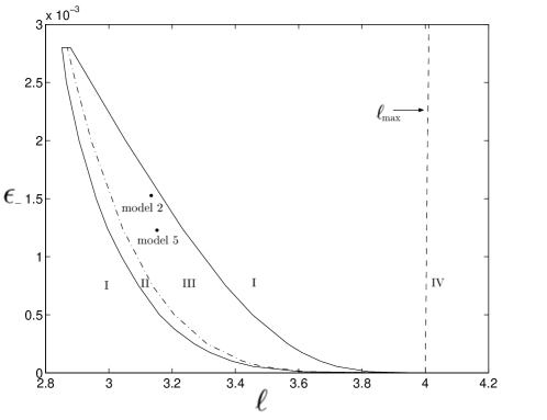
Figure 2: Plot of the $(\epsilon_{-},\ell)$ parameter space for an ADAF disk with $\gamma=1.5$. Only smooth flows exist in region I, and both shocked and smooth solutions are possible in regions II and III. When $\ell>\ell_{\rm max}$ (region IV), no steady-state dynamical solutions can be developed. The parameters corresponding to models 2 and 5 are indicated.

Equations (4), (8), and (13) can be combined with equations (30), (33), and (34) to obtain

$$\rho_{+}v_{+}a_{+} = \rho_{-}v_{-}a_{-}\ ,$$ (35)

$$a_{+}P_{+}-a_{-}P_{-} = a_{-}\rho_{-}v_{-}^{2}-a_{+}\rho_{+}v_{+}^{2}\ ,$$ (36)

$$\epsilon_{{}_{+}}-\epsilon_{{}_{-}} = {v_{+}^{2}-v_{-}^{2}\over 2}+{a_{+}^{2}-a_{-}^{2}\over\gamma-1}\ ,$$ (37)

where the subscripts “-” and “+” refer to quantities measured just upstream and just downstream from the shock, respectively. In the case of an isothermal shock, $a_{+}=a_{-}$, and therefore the shock jump conditions reduce to

$$\rho_{+}v_{+} = \rho_{-}v_{-}\ ,$$ (38)

$$P_{+}-P_{-} = \rho_{-}v_{-}^{2}-\rho_{+}v_{+}^{2}\ ,$$ (39)

$$\epsilon_{+}-\epsilon_{-} = {v_{+}^{2}-v_{-}^{2}\over 2}\ .$$ (40)

Combining equations (38) and (39) and substituting for the pressure $P$ using equation (9) yields the velocity jump condition

$${v_{+}\over v_{-}}=\gamma^{-1}\,{\cal M}_{-}^{-2}\ <\ 1\ ,\ \ \ \ \ {\cal M}_{-}\equiv{v_{-}\over a_{-}}\ ,$$ (41)

where ${\cal M}_{-}$ is the incident Mach number of the shock. The corresponding result for the shock compression ratio $R_{*}$ is

$$R_{*}\equiv{\rho_{+}\over\rho_{-}}=\gamma\,{\cal M}_{-}^{2}\ \ >\ \ 1\ .$$ (42)

Hence the gas density increases across the shock as expected. Based on equations (15) and (41) and the fact that $a_{+}=a_{-}$ in an isothermal shock, we find that the jump condition for the entropy parameter $K$ is given by

$${K_{+}\over K_{-}}=\gamma^{-1}\,{\cal M}_{-}^{-2}\ <\ 1\ ,$$ (43)

which indicates that entropy is lost from the disk at the shock location due to the escape of the particles that form the outflow (jet).

We can also make use of equation (41) to rewrite the jump condition for the energy transport parameter (eq. [40]) as

$$\Delta\epsilon\equiv\epsilon_{+}-\epsilon_{-}={v_{-}^{2}\over 2}\,\left({1\over\gamma^{2}{\cal M}_{-}^{4}}-1\right)\ <\ 0\ .$$ (44)

The associated rate at which energy escapes from the disk at the isothermal shock location (the “shock luminosity”) is given by (see eq. [13])

$$L_{\rm shock}\equiv-\Delta\dot{E}=-\dot{M}\,\Delta\epsilon\ \ \propto\ {\rm ergs\ s}^{-1}\ .$$ (45)

Eliminating $\Delta\epsilon$ between equations (44) and (45) yields the alternative result

$${L_{\rm shock}\over\dot{M}}={v_{-}^{2}\over 2}\,\left(1-{1\over\gamma^{2}{\cal M}_{-}^{4}}\right)\ .$$ (46)

4.2 Shock Point Analysis

For a given value of $\gamma$, it is known that smooth, shock-free global flow solutions exist only within a restricted region of the $(\epsilon_{-},\ell)$ parameter space, and isothermal shocks can occur only in a subset of the smooth-flow region. In order for a shock to exist in the flow, it must be located between two critical points, and it must also satisfy the jump conditions given by equations (41), (43), and (44). The procedure for determining the disk/shock structure is summarized below.

The process begins with the selection of values for the fundamental parameters $\epsilon_{-}$, $\ell$, and $\gamma$. The values of $\epsilon_{-}$ and $\ell$ are ultimately constrained by the observations of a specific object, as discussed in § 7. Following Narayan, Kato, & Honma (1997), we shall assume an approximate equipartition between the gas and magnetic pressures, and therefore we set $\gamma=1.5$. The first step in the determination of the shock location is the computation of the outer critical point location, $r_{c1}$, using the quartic equation (27). The associated values for the critical velocity, $v_{c1}$, the critical sound speed, $a_{c1}$, and the critical entropy, $K_{c1}$, are then calculated using equations (23), (24), and (25), respectively. Note that since the flow is adiabatic everywhere in the pre-shock region, it follows that

$$K_{-}=K_{c1}\ .$$ (47)

The profiles of the velocity $v(r)$ and the sound speed $a(r)$ in the pre-shock region can therefore be calculated using a root-finding procedure based on equation (29), or, alternatively, by integrating numerically the wind equation (19). The next step is the selection of an initial guess for the shock radius, $r_{*}$, and the calculation of the associated shock Mach number ${\cal M}_{-}\equiv v_{-}/a_{-}$ using the pre-shock dynamical solutions for $v(r)$ and $a(r)$. Based on the value of ${\cal M}_{-}$, we can compute the jump in the entropy parameter $K$ using equation (43), and consequently we find that the entropy in the downstream region is given by

$$K_{+}={K_{c1}\over\gamma\,{\cal M}_{-}^{2}}\ ,$$ (48)

where we have also used equation (47).

In order to determine whether the initial guess for $r_{*}$ is self-consistent, we employ a second, independent procedure for calculating the entropy in the downstream region based on the critical nature of the flow. In this approach, the downstream energy parameter $\epsilon_{+}$ is calculated using the jump condition given by equation (44), which yields

$$\epsilon_{+}=\epsilon_{-}+{v_{-}^{2}\over 2}\,\left({1\over\gamma^{2}{\cal M}_{-}^{4}}-1\right)\ .$$ (49)

We utilize this value to compute the downstream critical point radius $\hat{r}_{c3}$ based on the quartic equation (27). The associated values for the critical velocity, $\hat{v}_{c3}$, the critical sound speed, $\hat{a}_{c3}$, and the critical entropy, $\hat{K}_{c3}$, are then calculated using equations (23), (24), and (25), respectively. The final step is to compare the value of $\hat{K}_{c3}$ with that obtained for $K_{+}$ using equation (48). If these two quantities are equal, then the shock radius $r_{*}$ is correct and the disk/shock model is therefore dynamically self-consistent. Otherwise, the value for $r_{*}$ must be iterated and the search continued. Roots for $r_{*}$ can be found only in certain regions of the $(\epsilon_{-},\ell,\gamma)$ parameter space, as discussed below.

By combining the analysis of the shock location discussed above with the critical conditions developed in § 3, we are able to compute the structure of shocked and shock-free (smooth) disk solutions for a given set of parameters $\epsilon_{-}$, $\ell$, and $\gamma$. The resulting topology of the parameter space is depicted in Figure 2 for the case with $\gamma=1.5$, which is the main focus of this paper. Within region I, only smooth flows are possible, and in regions II and III both smooth and shocked solutions are available. No global flow solutions (either smooth or shocked) exist in region IV, with $\ell>\ell_{\rm max}$. Inside region II, one root for the shock radius $r_{*}$ can be found, and in region III two shock solutions are available, although only one actual shock can occur in a given flow. It is unclear which of the two roots for $r_{*}$ in region III is preferred since the stability properties of the shocks are not completely understood (e.g., Chakrabarti 1989a, 1989b; Abramowicz & Chakrabarti 1990). However, it is worth noting that the inner shock is always the stronger of the two because the Mach number diverges as the gas approaches the horizon. The larger compression ratio associated with the inner location leads to more efficient particle acceleration and enhanced entropy generation, and therefore we expect that the inner solution is preferred in nature. Based on this argument, we will focus on the inner shock location in our subsequent analysis.

Before we proceed to examine the transport equation for the relativistic particles, it is important to analyze the asymptotic solutions obtained for the dynamical variables near the event horizon and also at large radii. This is a crucial issue since the nature of the global solutions to the transport equation depends sensitively on the boundary conditions imposed at large and small radii. The asymptotic solutions for the dynamical variables near the event horizon were fully discussed by Becker & Le (2003). We shall briefly review their results and then perform a similar analysis in order to determine the asymptotic properties of the solutions as $r\to\infty$.

4.3 Asymptotic Behavior Near the Horizon

Becker & Le (2003) demonstrated that the variation of the global solutions in a viscous ADAF disk becomes purely adiabatic close to the event horizon, and therefore the asymptotic solutions that they obtain can be directly applied to our inviscid model. Using their equations (47) and (51), we find that the asymptotic variations of the radial velocity $v$ and the sound speed $a$ near the horizon are given by

$$v^{2}(r)\propto(r-r_{{}_{\rm S}})^{-1}\ ,\ \ \ \ \ \ \ a^{2}(r)\propto(r-r_{{}_{\rm S}})^{(1-\gamma)/(1+\gamma)}\ ,\ \ \ \ \ r\to r_{{}_{\rm S}}\ .$$ (50)

The divergence of $v$ as $r\to r_{{}_{\rm S}}$ implies that it cannot represent the standard velocity in the region near the horizon. However, our dynamical model is consistent with relativity if we interpret $v$ as the radial component of the four-velocity in this region (Becker & Le 2003; Becker & Subramanian 2005). By combining these relations with equations (4), (8), and (10), we find that the corresponding results for the asymptotic variations of the disk half-thickness $H$ and the density $\rho$ become

$$H(r)\propto(r-r_{{}_{\rm S}})^{(\gamma+3)/(2\gamma+2)}\ ,\ \ \ \ \ \ \ \rho(r)\propto(r-r_{{}_{\rm S}})^{-1/(\gamma+1)}\ ,\ \ \ \ \ r\to r_{{}_{\rm S}}\ .$$ (51)

4.4 Asymptotic Behavior at Infinity

We can use the energy transport equation (13) and the entropy equation (15) to obtain the asymptotic solutions for $v$ and $a$ at infinity as follows. In the limit $r\to\infty$, the two dominant terms in equation (13) are $\epsilon$ and $a^{2}/(\gamma-1)$, and therefore we find that

$$a^{2}(r)\to(\gamma-1)\,\epsilon\ ,\ \ \ \ \ r\to\infty\ .$$ (52)

Recalling that $K$ is constant in the adiabatic upstream flow, we can combine equations (15) and (52) to conclude that the asymptotic variation of the inflow velocity is given by

$$v\propto r^{-5/2}\ ,\ \ \ \ \ r\to\infty\ .$$ (53)

Finally, based on equations (8), (10), and (52), we find that the disk half-height varies as

$$H\propto r^{3/2}\ ,\ \ \ \ \ r\to\infty\ .$$ (54)

We can also combine equations (9), (14), and (52) to conclude that the asymptotic behavior of the density is given by

$$\rho\to{\rm const.}\ ,\ \ \ \ \ r\to\infty\ .$$ (55)

5 STEADY-STATE PARTICLE ACCELERATION

Our goal in this paper is to analyze the transport and acceleration of relativistic particles (ions) in a disk governed by the dynamical model developed in § 3 – 4. For fixed values of the theory parameters $\epsilon_{-}$, $\ell$, and $\gamma$, we will study the transport of particles in disks with and without shocks. The particle transport model utilized here includes advection, spatial diffusion, Fermi energization, and particle escape. In order to maintain consistency with the dynamics of the disk, we will need to equate the energy escape rate for the relativistic particles with the “shock luminosity” $L_{\rm shock}$ given by equation (45). Our treatment of Fermi energization includes both the general compression related to the overall convergence of the accretion flow, as well as the enhanced compression that occurs at the shock. In the scenario under consideration here, the escape of particles from the disk occurs via vertical spatial diffusion in the tangled magnetic field, as depicted in Figure 1. To avoid unnecessary complexity, we will utilize a simplified model in which only the radial ($r$) component of the spatial particle transport is treated in detail. In this approach, the diffusion and escape of the particles in the vertical ($z$) direction is modeled using an escape-probability formalism. We will treat the relativistic ions as test particles, meaning that their contribution to the pressure in the flow is neglected. This assumption is valid provided the pressure of the relativistic particles turns out to be a small fraction of the thermal pressure, as discussed in § 8. The ions accelerated at the shock are energized via collisions with MHD waves advected along with the background (thermal) flow, and therefore the shock width is expected to be comparable to the magnetic coherence length, $\lambda_{\rm mag}$. This approximation will be used to determine the rate at which particles escape from the disk in the vicinity of the shock.

5.1 Transport Equation

The Green’s function, $f_{{}_{\rm G}}(E_{0},E,r_{*},r)$, represents the particle distribution resulting from the continual injection of $\dot{N}_{0}$ particles per second, each with energy $E_{0}$, from a source located at the shock radius, $r=r_{*}$. In a steady-state situation, the Green’s function satisfies the transport equation (Becker 1992)

$${\partial f_{{}_{\rm G}}\over\partial t}=0=-\vec{\nabla}\cdot\vec{F}-{1\over 3E^{2}}{\partial\over\partial E}\left(E^{3}\vec{v}\cdot\vec{\nabla}f_{{}_{\rm G}}\right)+\dot{f}_{\rm source}-\dot{f}_{\rm esc}\ ,$$ (56)

where the specific flux $\vec{F}$ is evaluated using

$$\vec{F}=-\kappa\vec{\nabla}f_{{}_{\rm G}}-{\vec{v}E\over 3}{\partial f_{{}_{\rm G}}\over\partial E}\ ,$$ (57)

and the source and escape terms are given by

$$\dot{f}_{\rm source}={\dot{N}_{0}\,\delta(E-E_{0})\,\delta(r-r_{*})\over(4\pi E_{0})^{2}\,r_{*}\,H_{*}}\ ,\ \ \ \ \dot{f}_{\rm esc}=A_{0}\,c\,\delta(r-r_{*})\,f_{{}_{\rm G}}\ .$$ (58)

The quantities $E$, $\kappa$, $\vec{v}$, and $H_{*}\equiv H(r_{*})$ represent the particle energy, the spatial diffusion coefficient, the vector velocity, and the disk half-thickness at the shock location, respectively, and the dimensionless parameter $A_{0}$ determines the rate of particle escape through the surface of the disk at the shock location. The vector velocity $\vec{v}$ has components given by $\vec{v}=v_{r}\hat{r}+v_{z}\hat{z}+v_{\phi}\,\hat{\phi}$, where $v=-v_{r}$ is the positive inflow speed.

The total number and energy densities of the relativistic particles, denoted by $n_{r}$ and $U_{r}$, respectively, are related to the Green’s function via

$$n_{r}(r)=\int_{0}^{\infty}4\pi E^{2}\,f_{{}_{\rm G}}\,dE\ ,\ \ \ \ \ U_{r}(r)=\int_{0}^{\infty}4\pi E^{3}\,f_{{}_{\rm G}}\,dE\ ,$$ (59)

which determine the normalization of $f_{{}_{\rm G}}$. Equations (56) and (57) can be combined to obtain the alternative form

$$\vec{v}\cdot\vec{\nabla}f_{{}_{\rm G}}={\vec{\nabla}\cdot\vec{v}\over 3}\,E\,{\partial f_{{}_{\rm G}}\over\partial E}+\vec{\nabla}\cdot\left(\kappa\,\vec{\nabla}f_{{}_{\rm G}}\right)+\dot{f}_{\rm source}-\dot{f}_{\rm esc}\ ,$$ (60)

where the left-hand side represents the co-moving (advective) time derivative and the terms on the right-hand side describe first-order Fermi acceleration, spatial diffusion, the particle source, and the escape of particles from the disk at the shock location, respectively. Note that escape and particle injection are localized to the shock radius due to the presence of the $\delta$-functions in equations (58). Our focus here is on the first-order Fermi acceleration of relativistic particles at a standing shock in an accretion disk, and therefore equation (60) does not include second-order Fermi processes that may also occur in the flow due to MHD turbulence (e.g., Schlickeiser 1989a,b; Subramanian, Becker, & Kazanas 1999).

Under the assumption of cylindrical symmetry, equations (58) and (60) can be rewritten as

$$v_{r}{\partial f_{{}_{\rm G}}\over\partial r}+v_{z}{\partial f_{{}_{\rm G}}\over\partial z} - {1\over 3}\left[{1\over r}{\partial\over\partial r}\left(rv_{r}\right)+{dv_{z}\over dz}\right]E{\partial f_{{}_{\rm G}}\over\partial E}-{1\over r}{\partial\over\partial r}\left(r\kappa{\partial f_{{}_{\rm G}}\over\partial r}\right)$$ (61)

$$= {\dot{N}_{0}\,\delta(E-E_{0})\,\delta(r-r_{*})\over(4\pi E_{0})^{2}\,r_{*}\,H_{*}}-A_{0}\,c\,\delta(r-r_{*})\,f_{{}_{\rm G}}\ ,$$

where the escape of particles from the disk is described by the final term on the right-hand side. In Appendix A, we demonstrate that the vertically integrated transport equation is given by (see eq. [A9])

$$Hv_{r}{\partial f_{{}_{\rm G}}\over\partial r} = {1\over 3r}{\partial\over\partial r}\left(rHv_{r}\right)E{\partial f_{{}_{\rm G}}\over\partial E}+{1\over r}{\partial\over\partial r}\left(rH\kappa{\partial f_{{}_{\rm G}}\over\partial r}\right)$$ (62)

$$+ {\dot{N}_{0}\,\delta(E-E_{0})\,\delta(r-r_{*})\over(4\pi E_{0})^{2}\,r_{*}}-A_{0}\,c\,H_{*}\,f_{{}_{\rm G}}\,\delta(r-r_{*})\ ,$$

where the symbols $f_{{}_{\rm G}}$, $v_{r}$, and $\kappa$ represent vertically averaged quantities. We establish in Appendix B that within the context of our one-dimensional spatial model, the dimensionless escape parameter $A_{0}$ appearing in equation (62) is given by (see eqs. [B8] and [B10])

$$A_{0}=\left({3\,\kappa_{*}\over c\,H_{*}}\right)^{2}\ <\ 1\ ,$$ (63)

where $\kappa_{*}\equiv(\kappa_{-}+\kappa_{+})/2$ denotes the mean value of the diffusion coefficient at the shock location. The condition $A_{0}<1$ is required for the validity of the diffusive picture we have employed in our model for the vertical transport.

5.2 Number and Energy Densities

The energy moments of the Green’s function, $I_{n}(r)$, are defined by

$$I_{n}(r)\equiv\int_{0}^{\infty}4\pi E^{n}\,f_{{}_{\rm G}}\,dE\ ,$$ (64)

so that (cf. eqs. [59])

$$n_{r}(r)=I_{2}(r)\ ,\ \ \ \ \ U_{r}(r)=I_{3}(r)\ .$$ (65)

By operating on equation (62) with $\int_{0}^{\infty}4\pi E^{n}\,dE$ and integrating by parts once, we find that the function $I_{n}$ satisfies the differential equation

$$Hv_{r}{dI_{n}\over dr} = -\left({n+1\over 3}\right){I_{n}\over r}\,{d\over dr}\left(rHv_{r}\right)+{1\over r}{d\over dr}\left(rH\kappa{dI_{n}\over dr}\right)$$ (66)

$$+ {\dot{N}_{0}\,E_{0}^{n-2}\,\delta(r-r_{*})\over 4\pi\,r_{*}}-A_{0}\,c\,H_{*}\,I_{n}\,\delta(r-r_{*})\ ,$$

which can be expressed in the flux-conservation form

$${d\over dr}\left(4\pi rHF_{n}\right)=4\pi rH\left[\left({2-n\over 3}\right)v{dI_{n}\over dr}+{\dot{N}_{0}\,E_{0}^{n-2}\,\delta(r-r_{*})\over 4\pi r_{*}H_{*}}-A_{0}\,c\,\delta(r-r_{*})\,I_{n}\right]\ ,$$ (67)

where $4\pi rHF_{n}$ represents the rate of transport of the $n$th moment, and the flux $F_{n}$ is defined by

$$F_{n}\equiv-\left({n+1\over 3}\right)v\,I_{n}-\kappa\,{dI_{n}\over dr}\ ,$$ (68)

and $v=-v_{r}$ denotes the positive inflow speed.

In order to close the system of equations and solve for the relativistic particle number and energy densities $I_{2}(r)$ and $I_{3}(r)$ using equation (66), we must also specify the radial variation of the diffusion coefficient $\kappa$. The behavior of $\kappa$ can be constrained by considering the fundamental physical principles governing accretion onto a black hole. First, we note that near the event horizon, particles are swept into the black hole at the speed of light, and therefore advection must dominate over diffusion. This condition applies to both the thermal (background) and the nonthermal (relativistic) particles. Second, we note that in the outer region ($r\to\infty$), diffusion is expected to dominate over advection. Focusing on the flux equation for the particle number density $n_{r}$, obtained by setting $n=2$ in equation (68), we can employ scale analysis to conclude based on our physical constraints that

$$\lim_{r\to r_{{}_{\rm S}}}{\kappa(r)\over(r-r_{{}_{\rm S}})\,v(r)}=0\ ,\ \ \ \ \ \ \ \ \ \ \ \lim_{r\to\infty}{r\,v(r)\over\kappa(r)}=0\ .$$ (69)

The precise functional form for the spatial variation of $\kappa$ is not completely understood in the accretion disk environment. In order to obtain a mathematically tractable set of equations with a reasonable physical behavior, we shall utilize the general form

$$\kappa(r)=\kappa_{0}\,v(r)\,r_{{}_{\rm S}}\left({r\over r_{{}_{\rm S}}}-1\right)^{\alpha}\ ,$$ (70)

where $\kappa_{0}$ and $\alpha$ are dimensionless constants. Due to the appearance of the inflow speed $v$ in equation (70), we note that $\kappa$ exhibits a jump at the shock. This is expected on physical grounds since the MHD waves that scatter the ions are swept along with the thermal background flow, and therefore they should also experience a density compression at the shock.

As discussed above, close to the event horizon, inward advection at the speed of light must dominate over outward diffusion. Conversely, in the outer region, we expect that diffusion will dominate over advection as $r\to\infty$. By combining equation (70) with the asymptotic velocity variations expressed by equations (50) and (53), we find that the conditions given by equations (69) are satisfied if $\alpha>1$, and in our work we set $\alpha=2$. Note that the escape parameter $A_{0}$ is related to $\kappa_{0}$ via equation (63), which can be combined with equation (70) to write

$$A_{0}=\left({3\kappa_{0}\,v_{*}r_{{}_{\rm S}}\over cH_{*}}\right)^{2}\left({r_{*}\over r_{{}_{\rm S}}}-1\right)^{4}<\,1\ ,$$ (71)

where $v_{*}\equiv(v_{-}+v_{+})/2$ represents the mean velocity at the shock location $r=r_{*}$. The value of the diffusion parameter $\kappa_{0}$ is constrained by the inequality in equation (71). In § 7 we demonstrate that $\kappa_{0}$ can be computed for a given source based on energy conservation considerations. With the introduction of equations (70) and (71), we have completely defined all of the quantities in the transport equation, and we can now solve for the number and energy densities of the relativistic particles. The particle distribution Green’s function $f_{{}_{\rm G}}$ and its applications will be discussed in a separate paper.

6 SOLUTIONS FOR THE ENERGY MOMENTS

Once the disk/shock dynamics have been computed based on the selected values for the free parameters $\epsilon_{-}$, $\ell,$ and $\gamma$ using the results in §§ 3 and 4, the associated solutions for the number and energy densities of the relativistic particles in the disk can be obtained by solving equation (66). In the case of the number density, $n_{r}=I_{2}$, an exact solution can be derived based on the linear first-order differential equation describing the conservation of particle flux. However, in order to understand the variation of the energy density, $U_{r}=I_{3}$, we must numerically integrate a second-order equation. The solutions obtained below are applied in § 7 to model the outflows observed in M87 and Sgr A${}^{*}\,$.

6.1 Relativistic Particle Number Density

The equation governing the transport of the particle number density, $n_{r}$, is obtained by setting $n=2$ in equation (67), which yields

$${d\dot{N}_{r}\over dr}=\dot{N}_{0}\,\delta(r-r_{*})-4\pi r_{*}H_{*}A_{0}\,c\,n_{r}\,\delta(r-r_{*})\ ,$$ (72)

where the relativistic particle transport rate, $\dot{N}_{r}(r)$, is defined by (cf. eq. [68])

$$\dot{N}_{r}(r)\equiv-4\pi rH\left(v\,n_{r}+\kappa\,{dn_{r}\over dr}\right)\ \propto\ {\rm s}^{-1}\ ,$$ (73)

and $\dot{N}_{r}>0$ if the transport is in the outward direction. Since the source is located at the shock, there are two spatial domains of interest in our calculation of the particle transport, namely domain I ($r>r_{*}$), and domain II ($r<r_{*}$). Note that the number density $n_{r}(r)$ must be continuous at $r=r_{*}$ in order to avoid generating an infinite diffusive flux according to equation (73). Away from the shock location, $r\neq r_{*}$, and therefore equation (72) reduces to $\dot{N}_{r}=\rm const.$, which reflects the fact that particle injection and escape are localized at the shock. We can therefore write

$$\dot{N}_{r}(r)=\cases{\dot{N}_{\rm I}\ ,&$r>r_{*}$ \ ,\cr\dot{N}_{\rm II}\ ,&$r<r_{*}$ \ ,\cr}$$ (74)

where the constant $\dot{N}_{\rm I}>0$ denotes the rate at which particles are transported outward, radially, from the source location, and the constant $\dot{N}_{\rm II}<0$ represents the rate at which particles are transported inward towards the event horizon.

The magnitude of the jump in the particle transport rate at the shock is obtained by integrating equation (72) with respect to radius in a very small region around $r=r_{*}$, which yields

$$\dot{N}_{\rm I}-\dot{N}_{\rm II}=\dot{N}_{0}-\dot{N}_{\rm esc}\ ,$$ (75)

where

$$\dot{N}_{\rm esc}\equiv 4\pi r_{*}H_{*}A_{0}\,c\,n_{*}$$ (76)

represents the (positive) rate at which particles escape from the disk at the shock location to form the outflow (jet), and $n_{*}\equiv n_{r}(r_{*})$. If no shock is present in the flow, then $A_{0}=0$ and therefore $\dot{N}_{\rm esc}$=0. Note that the discontinuity in $\dot{N}_{r}$ at the shock produces a jump in the derivative $dn_{r}/dr$ via equation (73).

We can rewrite equation (73) for the number density in the form

$${dn_{r}\over dr}+{v\over\kappa}\,n_{r}=-{\dot{N}_{r}\over 4\pi rH\kappa}\ ,$$ (77)

which is a linear, first-order differential equation for $n_{r}(r)$. Using the standard integrating factor technique and employing equation (70) for $\kappa$ yields the exact solution

$$n_{r}(r)=e^{-J(r)}\left[n_{*}-{\dot{N}_{r}(r)\over 4\pi}\int_{r_{*}}^{r}{e^{J(r^{\prime})}\over r^{\prime}H\kappa}\,dr^{\prime}\right]\ ,$$ (78)

where $\dot{N}_{r}(r)$ is given by equation (74) and the function $J(r)$ is defined by

$$J(r)\equiv\int_{r_{*}}^{r}v\kappa^{-1}\,dr^{\prime}=\kappa_{0}^{-1}\left[\left({r_{*}\over r_{{}_{\rm S}}}-1\right)^{-1}-\left({r\over r_{{}_{\rm S}}}-1\right)^{-1}\right]\ .$$ (79)

According to equation (78), $n_{r}(r)$ is continuous at the shock/source location as required. Far from the black hole, diffusion dominates the particle transport, and therefore $n_{r}$ should vanish as $r\to\infty$. In order to ensure this behavior, we must have

$$n_{*}=\dot{N}_{\rm I}\,C_{\rm I}\ ,$$ (80)

where

$$C_{\rm I}\equiv{1\over 4\pi}\int_{r_{*}}^{\infty}{e^{J(r^{\prime})}\over r^{\prime}H\kappa}\,dr^{\prime}\ .$$ (81)

Furthermore, in order to avoid exponential divergence of $n_{r}$ as $r\to r_{{}_{\rm S}}$ in domain II, we also require that

$$n_{*}=-\dot{N}_{\rm II}\,C_{\rm II}\ ,$$ (82)

where

$$C_{\rm II}\equiv{1\over 4\pi}\int_{r_{{}_{\rm S}}}^{r_{*}}{e^{J(r^{\prime})}\over r^{\prime}H\kappa}\,dr^{\prime}\ .$$ (83)

By combining equations (75), (76), (80), and (82), we can develop explicit expressions for the quantities $n_{*}$, $\dot{N}_{\rm I}$, $\dot{N}_{\rm II}$, and $\dot{N}_{\rm esc}$ based on the values of $r_{*}$ and $\dot{N}_{0}$ and the profiles of the inflow velocity $v(r)$ and the diffusion coefficient $\kappa(r)$. The results obtained are

$$n_{*} = {\dot{N}_{0}\over C_{\rm I}^{-1}+C_{\rm II}^{-1}+4\pi r_{*}H_{*}A_{0}\,c}\ ,$$

$$\dot{N}_{\rm I} = {n_{*}\over C_{\rm I}}\ ,$$ (84)

$$\dot{N}_{\rm II} = -{n_{*}\over C_{\rm II}}\ ,$$

$$\dot{N}_{\rm esc} = 4\pi r_{*}H_{*}A_{0}\,c\,n_{*}\ .$$

These relations, along with equation (78), complete the formal solution for the relativistic particle number density $n_{r}(r)$. The solution is valid in both shocked and shock-free disks (the shock-free case is treated by setting $A_{0}=0$). When a shock is present, the particle escape rate $\dot{N}_{\rm esc}$ is proportional to $\dot{N}_{0}$ but is independent of $E_{0}$ by virtue of equations (84).

It is interesting to examine the asymptotic variation of $n_{r}$ near the event horizon and also at large distances from the black hole. Far from the hole, advection is negligible and the particle transport in the disk is dominated by outward-bound diffusion. In this case we can use equation (77) to conclude that

$${dn_{r}\over dr}\to-{\dot{N}_{\rm I}\over 4\pi rH\kappa}\ ,\ \ \ \ \ \ \ r\to\infty\ ,$$ (85)

where we have used the fact that $\dot{N}_{r}=\dot{N}_{\rm I}$ for $r>r_{*}$. By combining equations (70) and (85) with the asymptotic relations given by equations (53) and (54), we find upon integration that

$$n_{r}(r)\propto{1\over r}\ ,\ \ \ \ \ \ \ r\to\infty\ .$$ (86)

In order to study the behavior of $n_{r}$ near the event horizon, we take the limit as $r\to r_{{}_{\rm S}}$ in equation (78), obtaining after some algebra

$$n_{r}(r)\to-{\dot{N}_{\rm II}\over 4\pi rHv}\ ,\ \ \ \ \ r\to r_{{}_{\rm S}}\ ,$$ (87)

where we have set $\dot{N}_{r}=\dot{N}_{\rm II}$. Comparing this relation with equation (4), we find that

$$n_{r}(r)\ \propto\ \rho(r)\ ,\ \ \ \ \ \ \ \quad r\to r_{{}_{\rm S}}\ ,$$ (88)

where $\rho$ is the density of the background (thermal) gas. Equation (88) is a natural consequence of the fact that the particle transport near the horizon is dominated by inward-bound advection. We can also combine equations (51) and (88) to obtain the explicit asymptotic form

$$n_{r}(r)\ \propto(r-r_{{}_{\rm S}})^{-1/(\gamma+1)}\ ,\ \ \ \ \ \ \ \quad r\to r_{{}_{\rm S}}\ .$$ (89)

6.2 Relativistic Particle Energy Density

The differential equation satisfied by the relativistic particle energy density, $U_{r}=I_{3}$, is obtained by setting $n=3$ in equation (66), which yields

$$Hv_{r}{dU_{r}\over dr} = -{4\over 3}\,{U_{r}\over r}\,{d\over dr}\left(rHv_{r}\right)+{1\over r}{d\over dr}\left(rH\kappa{dU_{r}\over dr}\right)$$ (90)

$$+ {\dot{N}_{0}\,E_{0}\,\delta(r-r_{*})\over 4\pi\,r_{*}}-A_{0}\,c\,H_{*}\,U_{r}\,\delta(r-r_{*})\ .$$

By analogy with equations (72) and (73), we can recast this expression in the flux-conservation form

$${d\dot{E}_{r}\over dr}=4\pi rH\left[-{v\over 3}{dU_{r}\over dr}+{\dot{N}_{0}\,E_{0}\,\delta(r-r_{*})\over 4\pi r_{*}H_{*}}-A_{0}\,c\,U_{r}\,\delta(r-r_{*})\right]\ ,$$ (91)

where the relativistic particle energy transport rate, $\dot{E}_{r}(r)$, is defined by

$$\dot{E}_{r}(r)\equiv-4\pi rH\left({4\over 3}\,v\,U_{r}+\kappa\,{dU_{r}\over dr}\right)\ \propto\ {\rm ergs\ s}^{-1}\ ,$$ (92)

and $\dot{E}_{r}>0$ for outwardly directed transport. Note that unlike the number transport rate $\dot{N}_{r}$, the energy transport rate $\dot{E}_{r}$ does not remain constant within domains I and II due to the appearance of the first term on the right-hand side of equation (91), which expresses the compressional work done on the relativistic particles by the background flow.

Although the energy density $U_{r}$ must be continuous at the shock/source location in order to avoid generating an infinite diffusive flux, the derivative $dU_{r}/dr$ displays a discontinuity at $r=r_{*}$, which is related to the jump in the energy transport rate via equation (92). By integrating equation (91) in a very small region around $r=r_{*}$, we find that

$$\Delta\dot{E}_{r}=L_{\rm esc}-\dot{N}_{0}\,E_{0}\ ,$$ (93)

where

$$L_{\rm esc}\equiv 4\pi r_{*}H_{*}A_{0}\,c\,U_{*}\ \propto\ {\rm ergs\ s}^{-1}$$ (94)

denotes the rate of escape of energy from the disk into the outflow (jet) at the shock location, and $U_{*}\equiv U_{r}(r_{*})$. If no shock is present, then $A_{0}=0$ and therefore $L_{\rm esc}=0$. We remind the reader that the symbol “$\Delta$” refers to the difference between post- and pre-shock quantities (see eq. [30]). Equations (92) and (93) can be combined to show that the derivative jump is given by

$$\Delta\left(\kappa\,{dU_{r}\over dr}\right)={\dot{N}_{0}\,E_{0}-L_{\rm esc}\over 4\pi r_{*}H_{*}}-{4\over 3}\,U_{*}\,\Delta v\ .$$ (95)

The differential equation (90) governing the relativistic particle energy density is second-order in radius, and therefore we will need to establish two boundary conditions in order to solve for $U_{r}(r)$. These can be obtained by analyzing the behavior of $U_{r}$ close to the event horizon and at large distances from the black hole. Far from the hole, advection is negligible and the particle transport in the disk is dominated by outward-bound diffusion. In this regime, Fermi acceleration is negligible, and consequently we find that $U_{r}\propto n_{r}$. We can therefore use equation (86) to conclude that

$$U_{r}(r)\propto{1\over r}\ ,\ \ \ \ \ \ \ r\to\infty\ .$$ (96)

Close to the event horizon, the particle transport is dominated by advection, and therefore $U_{r}$ and $n_{r}$ obey the standard adiabatic relation

$$U_{r}\propto n_{r}^{4/3}\ ,\ \ \ \ \ \ \ r\to r_{{}_{\rm S}}\ .$$ (97)

Combining this result with equations (88) then yields

$$U_{r}\propto(r-r_{{}_{\rm S}})^{-4/(3\gamma+3)}\ ,\ \ \ \ \ \ \ r\to r_{{}_{\rm S}}\ .$$ (98)

The global solution for $U_{r}(r)$ can now be expressed as

$$U_{r}(r)=\cases{A\ Q_{\rm I}(r)\ ,&$r>r_{*}$ \ ,\cr B\ Q_{\rm II}(r)\ ,&$r<r_{*}$ \ ,\cr}$$ (99)

where $A$ and $B$ are constants and the functions $Q_{\rm I}(r)$ and $Q_{\rm II}(r)$ satisfy the homogeneous differential equation (see eq. [90])

$$Hv_{r}{dQ\over dr}=-{4\over 3}\,{Q\over r}\,{d\over dr}\left(rHv_{r}\right)+{1\over r}{d\over dr}\left(rH\kappa{dQ\over dr}\right)\ .$$ (100)

along with the boundary conditions (see eqs. [96] and [98])

$$Q_{\rm I}(r_{\rm out})=\left({r_{\rm out}\over r_{{}_{\rm S}}}\right)^{-1}\ ,\ \ \ \ \ \ \ Q_{\rm II}(r_{\rm in})=\left({r_{\rm in}\over r_{{}_{\rm S}}}-1\right)^{-4/(3\gamma+3)}\ ,$$ (101)

where $r_{\rm in}$ and $r_{\rm out}$ denote the radii at which the inner and outer boundary conditions are applied, respectively. The constants $A$ and $B$ are computed by requiring that $U_{r}$ be continuous at $r=r_{*}$ and that the derivative $dU_{r}/dr$ satisfy the jump condition given by equation (95). The results obtained are

$$A = B\,{Q_{\rm II}\over Q_{\rm I}}\Bigg{|}_{r=r_{*}}\ ,$$ (102)

$$B = {\dot{N}_{0}\,E_{0}\over 4\pi r_{*}H_{*}}\Bigg{[}{4\over 3}\,(v_{-}-v_{+})\,Q_{\rm II}+Q_{\rm II}^{\prime}\kappa_{+}-{Q_{\rm II}Q_{\rm I}^{\prime}\kappa_{-}\over Q_{\rm I}}+A_{0}\,c\,Q_{\rm II}\Bigg{]}^{-1}\Bigg{|}_{r=r_{*}}\ ,$$ (103)

where primes denote differentiation with respect to radius. The solutions for the functions $Q_{\rm I}(r)$ and $Q_{\rm II}(r)$ are obtained by integrating numerically equation (100) subject to the boundary conditions given by equations (101). Once the constants $A$ and $B$ are computed using equations (102) and (103), the global solution for $U_{r}(r)$ is evaluated using equation (99). The solution applies whether or not a shock is present in the flow. The shock-free case is treated by setting $A_{0}=0$. This completes the solution procedure for the relativistic particle energy density. The results derived in this section are used in § 7 to model the outflows observed in M87 and Sgr A${}^{*}\,$.

7 ASTROPHYSICAL APPLICATIONS

Our goal is to determine the properties of the integrated disk/shock/outflow model based on the observed values for the black hole mass $M$, the mass accretion rate $\dot{M}$, and the jet kinetic power $L_{\rm jet}$ associated with a given source. The fundamental free parameters for the theoretical model are $\epsilon_{-}$, $\ell$, and $\gamma$. Since we set $\gamma=1.5$ in order to represent an approximate equipartition between the gas and magnetic pressures (e.g., Narayan, Kato, & Honma 1997), only $\epsilon_{-}$ and $\ell$ remain to be determined. Here we describe how global energy conservation considerations can be used to solve for the various theoretical parameters in the model based on observations.

7.1 Energy Conservation Conditions

Once the values of $M$, $\dot{M}$, and $L_{\rm jet}$ have been specified for a source based on observations, we select a value for the free parameter $\epsilon_{-}$ and then compute $\ell$ by satisfying the relation

$$L_{\rm shock}=L_{\rm jet}\ ,$$ (104)

where $L_{\rm shock}$ is the shock luminosity given by equation (46). This result ensures that the jump in the energy transport rate at the isothermal shock location is equal to the observed jet kinetic luminosity. The procedure for determining $\ell$ also includes solving for the shock location and the critical structure using results from §§ 3 and 4. The velocity profile $v(r)$ is computed either by numerically integrating equation (19) or by using a root-finding procedure based on equation (29), and the associated solution for the adiabatic sound speed $a(r)$ is obtained using equation (13).

After the velocity profile has been determined, we can compute the number and energy density distributions for the relativistic particles in the disk using equations (78) and (99), respectively. This requires the specification of the injection energy of the seed particles $E_{0}$ as well as their injection rate $\dot{N}_{0}$. We set the injection energy using $E_{0}=0.002\,$ergs, which corresponds to an injected Lorentz factor $\Gamma_{0}\equiv E_{0}/(m_{p}\,c^{2})\sim 1.3$, where $m_{p}$ is the proton mass. Particles injected with energy $E_{0}$ are subsequently accelerated to much higher energies due to repeated shock crossings. We find that the speed of the injected particles, $v_{0}=c\,(1-\Gamma_{0}^{-2})^{1/2}$, is about three to four times higher than the mean ion thermal velocity at the shock location, $v_{\rm rms}=(3kT_{*}/m_{p})^{1/2}$, where $T_{*}$ is the ion temperature at the shock. The seed particles are therefore picked up from the high-energy tail of the Maxwellian distribution for the thermal ions. With $E_{0}$ specified, we can compute the particle injection rate $\dot{N}_{0}$ using the energy conservation condition

$$\dot{N}_{0}\,E_{0}=L_{\rm shock}\ ,$$ (105)

which ensures that the rate at which energy is injected into the flow in the form of the relativistic seed particles is equal to the energy loss rate for the background gas at the isothermal shock location.

In order to maintain agreement between the transport model and the observations, we must also require that the rate at which particle energy escapes from the disk due to vertical diffusion is equal to the observed jet power. This condition can be written as

$$L_{\rm esc}=L_{\rm jet}\ ,$$ (106)

where $L_{\rm esc}$ is the energy escape rate given by equation (94). The escape constant, $A_{0}$, appearing in the transport equation is independent of the particle energy in our model, and consequently the escaping particles will have exactly the same mean energy as those in the disk at the shock location. The mean energy of the escaping particles is therefore given by

$$E_{\rm esc}\equiv{U_{*}\over n_{*}}\ ,$$ (107)

where $n_{*}$ and $U_{*}$ denote the number and energy densities of the relativistic particles at the shock location, respectively. Hence $E_{\rm esc}$ is proportional to $E_{0}$ but it is independent of $\dot{N}_{0}$. We note that equations (76), (94), and (107) can be combined to show that

$$L_{\rm esc}=\dot{N}_{\rm esc}\,E_{\rm esc}\ ,$$ (108)

where $\dot{N}_{\rm esc}$ is the particle escape rate (eq. [76]). By satisfying equations (104), (105), and (106), we ensure that energy is properly conserved in our model. Taken together, these relations allow us to solve for the various theoretical parameters based on observational values for $M$, $\dot{M}$, and $L_{\rm jet}$, as explained below.

Table 1: Disk structure parameters

Model	$\epsilon_{{}_{-}}$	$\ell$	$\epsilon_{{}_{+}}$	$r_{c1}$	$r_{c3}$	$r_{*}$	$\hat{r}_{c3}$	$H_{*}$	${\cal M}_{*}$	$R_{*}$	$T_{*}$
1	0.001600	3.1040	-0.005676	93.177	5.478	19.624	5.798	10.369	1.094	1.795	1.28
2	0.001527	3.1340	-0.005746	98.524	5.379	21.654	5.659	11.544	1.125	1.897	1.16
3	0.001400	3.1765	-0.005875	109.781	5.252	24.500	5.487	13.154	1.170	2.052	1.01
4	0.001240	3.1280	-0.008723	131.204	5.408	14.073	5.850	6.819	1.113	1.857	1.65
5	0.001229	3.1524	-0.008749	131.874	5.329	15.583	5.723	7.672	1.146	1.970	1.49
6	0.001200	3.1756	-0.008778	135.192	5.260	16.950	5.614	8.434	1.177	2.076	1.36

All quantities are expressed in gravitational units ($GM=c=1$) except $T_{*}$ which is in units of $10^{11}\,$K.

7.2 Model Parameters

Our simulations of the disk structure and particle transport in M87 and Sgr A${}^{*}\,$are based on various published observational estimates for $M$, $\dot{M}$, and $L_{\rm jet}$. For M87, we set $M=3\times 10^{9}{\rm\ M_{\odot}}$ (e.g., Ford et al. 1994), $\dot{M}=1.3\times 10^{-1}{\rm\ M_{\odot}\ yr^{-1}}$ (e.g., Reynolds et al. 1996), and $L_{\rm jet}=5.5\times 10^{43}\,{\rm ergs\ s^{-1}}$ (e.g., Reynolds et al. 1996; Bicknell & Begelman 1996; Owen, Eilek, & Kassim 2000). For Sgr A${}^{*}\,$, we use the values $M=2.6\times 10^{6}{\rm\ M_{\odot}}$ (e.g., Schödel et al. 2002) and $\dot{M}=8.8\times 10^{-7}{\rm\ M_{\odot}\ yr^{-1}}$ (e.g., Yuan, Markoff, & Falcke 2002; Quataert 2003). Although the kinetic luminosity of the jet in Sgr A${}^{*}\,$is rather uncertain (see, e.g., Yuan 2000; Yuan et al. 2002), we will adopt the value quoted by Falcke & Biermann (1999), and therefore we set $L_{\rm jet}=5\times 10^{38}{\rm ergs\ s^{-1}}$.

We study both shocked and shock-free solutions spanning the computational domain between the inner radius $r_{\rm in}=2.001$ and the outer radius $r_{\rm out}=5000$, where $r_{\rm in}$ and $r_{\rm out}$ are the radii at which the boundary conditions are applied (see eqs. [101]). Six different accretion/shock scenarios are explored in detail, with the values for the various parameters $\epsilon_{-}$, $\ell$, $\epsilon_{+}$, $r_{c1}$, $r_{c3}$, $r_{*}$, $\hat{r}_{c3}$, $H_{*}$, ${\cal M}_{*}$, $R_{*}$, and $T_{*}$ reported in Table 1. Models 1, 2, and 3 are associated with M87, while models 4, 5, and 6 are used to study Sgr A${}^{*}\,$. In our numerical examples, we utilize natural gravitational units ($GM=c=1$ and $r_{{}_{\rm S}}=2$), except as noted. Based on the observational values for $\dot{M}$ and $L_{\rm jet}$ associated with the two sources, we can use equations (45) and (104) to conclude that $\Delta\epsilon=-0.007$ for M87 and $\Delta\epsilon=-0.01$ for Sgr A${}^{*}\,$. These results are consistent with the values for $\epsilon_{-}$ and $\epsilon_{+}$ reported in Table 1, and therefore $L_{\rm shock}=L_{\rm jet}$ as required (see eq. [104]).

Next we use the energy conservation condition $L_{\rm esc}=L_{\rm jet}$ (eq. [106]) to determine the value of the diffusion constant $\kappa_{0}$ (eq. [70]) for a shocked disk. In Figure 3, we plot $L_{\rm esc}/L_{\rm jet}$, $\Gamma_{\rm esc}$, and $\dot{N}_{\rm esc}/\dot{N}_{0}$ as functions of $\kappa_{0}$ for the M87 and Sgr A${}^{*}\,$parameters, where $\Gamma_{\rm esc}\equiv E_{\rm esc}/(m_{p}\,c^{2})$ is the mean Lorentz factor of the escaping particles. The treatment of energy conservation in our disk/shock model is self-consistent when the condition $L_{\rm esc}/L_{\rm jet}=1$ is satisfied, which corresponds to specific values of $\kappa_{0}$ as indicated in Figures 3a and 3d. We find that two $\kappa_{0}$ roots exist for models 3 and 6, one root is possible for models 2 and 5, and no roots exist for models 1 and 4. Hence the values of $\epsilon_{-}$ associated with models 2 and 5 represent the maximum possible values for $\epsilon_{-}$ that yield self-consistent solutions based on the M87 and Sgr A${}^{*}\,$data, respectively. For illustrative purposes, we shall focus on the details of the disk structure and particle transport obtained in models 2 and 5.

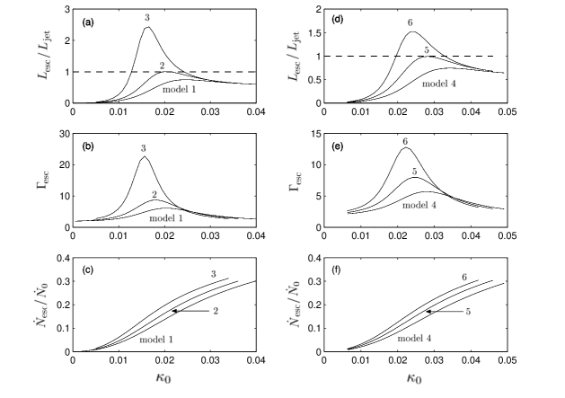
Figure 3: Quantities $L_{\rm esc}/L_{\rm jet}$, $\Gamma_{\rm esc}$, and $\dot{N}_{\rm esc}/\dot{N}_{0}$ for a shocked disk plotted as functions of $\kappa_{0}$. Panels (a), (b), and (c) correspond to the M87 parameters (models 1, 2 and 3), and panels (d), (e), and (f) correspond to the Sgr A${}^{*}\,$parameters (models 4, 5 and 6). The model numbers are indicated for each curve. See the discussion in the text.

Table 2: Transport equation parameters

Model	$\dot{N}_{0}$	$\underline{\dot{N}_{\rm I}}$	$\kappa_{0}$	$\kappa_{*}$	$A_{0}$	$n_{*}$	$U_{*}$	$\underline{\dot{N}_{\rm esc}}$	$\underline{E_{\rm esc}}$	$\Gamma_{\rm esc}$
	(s-1)	$\dot{N}_{\rm II}$				(cm-3)	(ergs cm-3)	$\dot{N}_{0}$	$E_{0}$
2	2.75 $\times 10^{46}$	-0.18	0.02044	0.427877	0.0124	$2.01\times 10^{4}$	$2.39\times 10^{2}$	$0.17$	5.95	7.92
5	2.51 $\times 10^{41}$	-0.15	0.02819	0.321414	0.0158	$4.33\times 10^{5}$	$4.71\times 10^{3}$	$0.18$	5.45	7.26

All quantities are expressed in gravitational units ($GM=c=1$) except as noted.

7.3 Disk Structure and Particle Transport

In order to illustrate the importance of the shock for the acceleration of high-energy particles, we shall examine the structure of the accretion disk either with and without a shock based on the values of the upstream parameters $\epsilon_{-}$ and $\ell$ utilized in models 2 and 5 (see Table 1). In Figures 4a and 4b we plot the inflow speed $v(r)$ and the adiabatic sound speed $a(r)$ for the shocked and smooth (shock-free) solutions associated with models 2 and 5, respectively. Since we are working within the isothermal shock scenario, the sound speed $a$ is continuous at the shock location. In Figures 4c and 4d we plot the specific internal energy $U/\rho=(\gamma-1)^{-1}kT/m_{p}$ for the background (thermal) gas along with the specific gravitational potential (binding) energy $GM/(r-r_{{}_{\rm S}})$ as functions of radius for $\gamma=1.5$. These results demonstrate that the gas is marginally bound in the absence of a shock, and strongly bound when a shock is present. The increased binding of the thermal gas in the disk results from the escape of energy in the outflow, which reduces the sound speed compared with the shock-free case. The enhanced cooling allows the accretion to proceed, thereby removing one of the major objections to the original ADAF scenario (Narayan & Yi 1994, 1995). We emphasize that these new results represent the first fully self-consistent calculations of the structure of an ADAF disk coupled with a shock-driven outflow, hence extending the heuristic work of Blandford & Begelman (1999) and Becker, Subramanian, & Kazanas (2001).

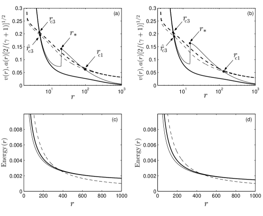
Figure 4: The velocity $v(r)$ (solid lines) and sound speed $a(r)\,[2/(\gamma+1)]^{1/2}$ (dashed lines) are plotted in units of $c$ for (a) model 2 and (b) model 5. The curves cross at the critical points. Also plotted are the specific internal energy $U/\rho$ (solid lines) and the specific gravitational potential energy $GM/(r-r_{{}_{\rm S}})$ (dashed lines), both in units of $c^{2}$, for (c) model 2 and (d) model 5. The shocked and shock-free solutions are denoted by the thin and heavy lines, respectively.

Next we study the solutions obtained for the relativistic particle number and energy density distributions in the disk based on the flow structures associated with models 2 and 5. The related transport parameters are listed in Table 2. In Figures 5 and 6 we plot the global number and energy density distributions obtained in a shocked disk using the model 2 and 5 parameters, respectively. We also include the corresponding results obtained in a shock-free (smooth) disk for the same values of the upstream energy transport rate $\epsilon_{-}$ and the specific angular momentum $\ell$. In each case the densities decrease monotonically with increasing radius. The increase near the horizon is a consequence of advection, while the decline as $r\to\infty$ reflects the fact that the particles injected at the shock have a very small chance of diffusing to large distances from the black hole. Note that the shocked disk has a lower value for the number density $n_{r}$ at all radii as a consequence of particle escape. However, the shocked disk also displays a higher value for the energy density $U_{r}$, which reflects the central role of shock in accelerating the relativistic test particles.

The kinks in the energy and number density distributions at the shock radius $r=r_{*}$ indicated in Figures 5 and 6 reflect the derivative jump conditions given by equations (75) and (95). The values for the ratios $\dot{N}_{\rm I}/\dot{N}_{\rm II}$ and $\dot{N}_{\rm esc}/\dot{N}_{0}$ reported in Table 2 indicate that most of the injected particles are advected into the black hole, with $\sim 20$% escaping to form the outflow (see Figs. 3c and 3f). In order to validate the accuracy of the numerical solutions for $n_{r}(r)$ and $U_{r}(r)$, we also compare the profiles obtained with the asymptotic relations developed in § 6. We demonstrate in Figure 7 (model 2) and Figure 8 (model 5) that the solutions for both $n_{r}(r)$ and $U_{r}(r)$ agree closely with the asymptotic expressions given by equations (89) and (98) for small radii and by equations (86) and (96) for large radii. Note that the values reported by Le & Becker (2004) for $n_{*}$ and $U_{*}$ were expressed in incorrect units and are given correctly in our Table 2.

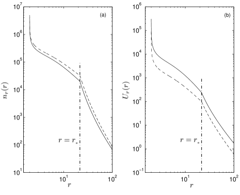
Figure 5: Global solutions for the relativistic number density (a) and the relativistic energy density (b) computed using the model 2 parameters. The solid and dashed curves correspond to disks with and without shocks, respectively. Note that the number density is higher in the smooth (shock-free) disk due to the absence of particle escape. Conversely, the energy density is higher in the shocked disk due to the enhanced particle acceleration occurring at the shock.

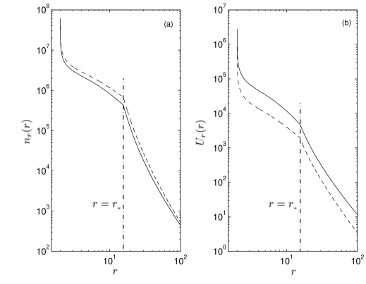
Figure 6: Same as Figure 5 but for model 5.

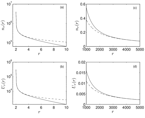
Figure 7: Plots of the numerical solutions for $n_{r}(r)$ and $U_{r}(r)$ (solid lines) computed using the model 2 parameters in a shocked disk are compared with the asymptotic expressions (dashed lines) close to the event horizon (a and b) and at large radii (c and d). See the discussion in the text.

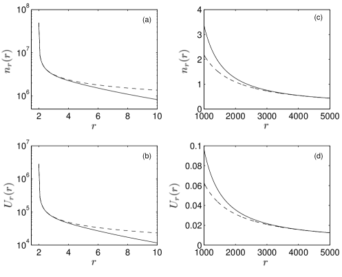
Figure 8: Same as Figure 7 but for model 5.

7.4 Jet Formation in M87 and Sgr A${}^{*}\,$

The mean energy of the relativistic particles in the disk is given by (cf. eq. [107])

$$\langle E\rangle\equiv{U_{r}(r)\over n_{r}(r)}\ ,$$ (109)

so that $\langle E\rangle=E_{\rm esc}$ at $r=r_{*}$. In Figure 9 we plot the mean energy as a function of radius in shocked and shock-free disks based on the parameters used for models 2 and 5. The results demonstrate that when a shock is present in the flow, the relativistic particle energy is boosted by a factor of $\sim 5-6$ at the shock location. By contrast, we find that in the shock-free models with the same values for $\epsilon_{-}$, $\ell$, and $\kappa_{0}$, the energy is boosted by a factor of only $\sim 1.4-1.5$. This clearly demonstrates the essential role of the shock in efficiently accelerating particles up to very high energies, far above the energy required to escape from the disk. Note that close to the event horizon, the mean energy of the relativistic particles is further enhanced by the strong compression of the accretion flow, as indicated by the sharp increase in $\langle E\rangle$ as $r\to r_{{}_{\rm S}}$.

The material in the outflow is initially ejected from the disk in the vicinity of the shock as a hot plasma which cools as it expands, with its outward acceleration powered by the pressure gradient in the surrounding plasma. Based on our results for models 2 and 5, we find that the shock/jet locations are given by $r_{*}\sim 22$ and $r_{*}\sim 16$ for M87 and Sgr A${}^{*}\,$, respectively. The terminal (asymptotic) Lorentz factor of the jet, $\Gamma_{\infty}$, can be estimated by writing

$$\Gamma_{\infty}=\Gamma_{\rm esc}={E_{\rm esc}\over m_{p}c^{2}}\ ,$$ (110)

which is based on the assumption that the jet starts off “slow” and “hot” and subsequently expands to become “fast” and “cold.” Adopting the $\Gamma_{\rm esc}$ values listed in Table 2 for M87 and Sgr A${}^{*}\,$, we obtain $\Gamma_{\infty}=7.92$ (see Fig. 3b) and $\Gamma_{\infty}=7.26$ (see Fig. 3e), respectively.

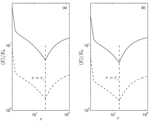
Figure 9: Mean energy of the relativistic particles in the disk, $\langle E\rangle\equiv U_{r}(r)/n_{r}(r)$ (eq. [109]), plotted in units of the injection energy $E_{0}$ as a function of radius for (a) model 2 and (b) model 5. Results are indicated for both shocked (solid lines) and shock-free (dashed lines) disk structures.

We can now compare our model predictions for the shock/jet location and the asymptotic Lorentz factor with the observations of M87 and Sgr A${}^{*}\,$. According to Biretta, Junor, & Livio (2002), the M87 jet forms in a region no larger than $\sim 30$ gravitational radii from the black hole, which agrees rather well with our predicted shock/jet location $r_{*}\sim 22$ for this source. Turning now to the asymptotic (terminal) Lorentz factor, we note that Biretta, Sparks, & Macchetto (1999) estimated $\Gamma_{\infty}\geq 6$ for the M87 jet, which is comparable to the result $\Gamma_{\rm\infty}=7.92$ obtained using our model. In the case of Sgr A${}^{*}\,$, our model indicates that the shock forms at $r_{*}\sim 16$ which is fairly close to the value suggested by Yuan (2000). However, future observational work will be needed to test our prediction for the asymptotic Lorentz factor of Sgr A${}^{*}\,$, since no reliable observational estimate for that quantity is currently available.

7.5 Radiative Losses from the Jet

It is still unclear whether the outflows observed to emanate from many radio-loud systems containing black holes are composed of an electron-proton plasma or electron-positron pairs, or a mixture of both. Whichever is the case, the particles must maintain sufficient energy during their journey from the nucleus in order to power the observed radio emission, unless some form of reacceleration takes place along the way, due to shocks propagating along the jet (e.g., Atoyan & Dermer 2004a). Proton-electron outflows, such as those studied here, have a distinct advantage in this regard since most of the kinetic power is carried by the ions, which do not radiate much and are not strongly coupled to the electrons under the typical conditions in a jet (e.g., Felten 1968; Felten, Arp, & Lynds 1970; Anyakoha et al. 1987; Aharonian 2002). We therefore suggest that if the observed outflows are proton-driven, then they may be powered directly by the shock acceleration mechanism operating in the disk, with no requirement for additional in situ reacceleration in the jet. In this section we confirm this conjecture by considering the energy losses experienced by the protons in the outflow. The ions in the jet lose energy via two distinct channels, namely (1) direct radiative losses due to the production of synchrotron and inverse-Compton emission, and (2) indirect radiative losses via Coulomb coupling with the electrons. We will evaluate these two possibilities by estimating the corresponding cooling timescales for the outflows in M87 and Sgr A${}^{*}\,$and comparing the results with the jet propagation timescales for these sources.

The energy loss rate due to the production of synchrotron and inverse-Compton emission by the relativistic protons escaping from the disk with mean energy $\Gamma_{\rm esc}m_{p}c^{2}$ is given by (see eqs. [7.17] and [7.18] from Rybicki & Lightman 1979)

$$\left(dE\over dt\right)\Bigg{|}_{\rm rad}={4\,\sigma_{{}_{\rm T}}c\,\Gamma^{2}_{\rm esc}\over 3}\left(m_{e}\over m_{p}\right)^{2}\left(U_{B}+U_{\rm ph}\right)\ ,$$ (111)

where $U_{\rm ph}$ and $U_{B}=B^{2}/(8\pi)$ denote the energy densities of the soft radiation and the magnetic field with strength $B$, respectively. The associated energy loss timescale is therefore

$$t_{\rm rad}\equiv{\Gamma_{\rm esc}m_{p}c^{2}\over~{}(dE/dt)\big{|}_{\rm rad}}={3\,m_{p}\,c\over 4\,\sigma_{{}_{\rm T}}\,\Gamma_{\rm esc}}\left(m_{p}\over m_{e}\right)^{2}\left(U_{B}+U_{\rm ph}\right)^{-1}\ .$$ (112)

In our application to M87, we take $B\sim 0.1\,$G based on estimates from Biretta, Stern, & Harris (1991), and we set $\Gamma_{\rm esc}\sim 8$ (see Table 2, model 2). Assuming equipartition between the magnetic field and the soft radiation, this yields for the radiative cooling time $t_{\rm rad}\sim 10^{12}\,$yrs, which suggests that the protons can easily maintain their energy for many millions of parsecs without being seriously effected by synchrotron or inverse-Compton losses, as expected. For Sgr A${}^{*}\,$, we assume equipartition with $B\sim 10\,$G (Atoyan & Dermer 2004b) and $\Gamma_{\rm esc}\sim 7$ (see Table 2, model 5). The radiative cooling time for the escaping protons is therefore $t_{\rm rad}\sim 10^{8}\,$yrs. Hence synchrotron and inverse-Compton losses have virtually no effect on the energy of the protons in the Sgr A${}^{*}\,$jet.

In addition to synchrotron and inverse-Compton radiation, the protons in the jet will also lose energy due to Coulomb coupling with the thermal electrons, which radiate much more efficiently than the protons. The energy loss rate for this process can be estimated using equation (4.16) from Mannheim & Schlickeiser (1994), which yields

$$\left(dE\over dt\right)\Bigg{|}_{\rm coul}=\,30\,n_{e}\,\sigma_{{}_{\rm T}}\,m_{e}c^{3}\ ,$$ (113)

where $n_{e}$ represents the electron number density in the jet. The associated loss timescale for a proton escaping from the disk with mean energy $\Gamma_{\rm esc}m_{p}c^{2}$ is

$$t_{\rm coul}\equiv{\Gamma_{\rm esc}m_{p}c^{2}\over~{}(dE/dt)\big{|}_{\rm coul}}={\Gamma_{\rm esc}\,m_{p}\over 30\,n_{e}\,\sigma_{{}_{\rm T}}\,c\,m_{e}}\ .$$ (114)

The electron number density $n_{e}$ decreases rapidly as the jet expands from the disk into the external medium. Hence the most conservative estimate (based on the strongest Coulomb coupling) is obtained by adopting conditions at the base of the jet, where $n_{e}$ has its maximum value. To estimate the electron number density at the base of the outflow, we begin by calculating the rate at which protons escape from the disk at the shock location. By using equation (B8) to eliminate $A_{0}$ in equation (76), we find that the proton escape rate is given by

$$\dot{N}_{\rm esc}={4\pi r_{*}\lambda_{\rm mag}^{2}\,c\,n_{*}\over H_{*}}\ ,$$ (115)

where $r_{*}$, $n_{*}$, $H_{*}$, and $\lambda_{\rm mag}$ denote the radius, the proton number density, the vertical half-thickness, and the magnetic mean free path inside the disk at the shock location, respectively. The shock is expected to have a width comparable to $\lambda_{\rm mag}$, and therefore the sum of the upper and lower face areas of the shock annulus is equal to $4\pi r_{*}\lambda_{\rm mag}$. We also note that the flux of the relativistic protons escaping from the disk into the outflow is given by $cn_{p}$, where $n_{p}$ is the proton number density at the base of the jet. Combining these relations, we can write the proton escape rate in terms of $n_{p}$ using

$$\dot{N}_{\rm esc}=4\pi r_{*}\lambda_{\rm mag}\,c\,n_{p}\ .$$ (116)

By equating the two expressions for $\dot{N}_{\rm esc}$ given by equations (115) and (116), we find that $n_{p}$ is related to $n_{*}$ via

$${n_{p}\over n_{*}}={\lambda_{\rm mag}\over H_{*}}\ <\ 1\ .$$ (117)

Since the electron-proton jet must be charge neutral, the electron number density at the base of the jet, $n_{e}$, is equal to the proton number density $n_{p}$, and therefore we obtain

$$n_{e}={\lambda_{\rm mag}\over H_{*}}\ n_{*}\ .$$ (118)

Using the relation $\lambda_{\rm mag}/H_{*}=A_{0}^{1/2}$ (see eq. [B8]) along with the results for $A_{0}$ and $n_{*}$ reported in Table 1 for M87 (model 2), we obtain $n_{e}=0.11\,n_{*}=2.2\times 10^{3}\,\rm cm^{-3}$. Setting $\Gamma_{\rm esc}\sim 8$, we find that equation (114) yields for the electron-proton Coulomb coupling timescale $t_{\rm coul}\sim 3.5\times 10^{5}\,$yrs. Note that this is an extremely conservative estimate since it is based on conditions at the bottom of the jet, and therefore it suggests that Coulomb coupling between the protons and the electrons is insufficient to seriously degrade the energy of the accelerated ions escaping from the disk as they propagate out to the radio lobes via the jet. For Sgr A${}^{*}\,$, we use the model 5 data in Table 2 to obtain $n_{e}=0.13\,n_{*}=5.6\times 10^{4}\,\rm cm^{-3}$. Setting $\Gamma_{\rm esc}\sim 7$ yields for the Coulomb coupling timescale $t_{\rm coul}\sim 1.2\times 10^{4}\,$yrs, which implies that the length of the jet can be as large several thousand parsecs before much energy is drained from the protons, assuming the material in the jet travels at half the speed of light. We emphasize that these numerical estimates of the importance of radiative and Coulomb losses experienced by the relativistic protons are based on the “worst-case” assumption that the conditions at the base of the outflow prevail throughout the jet. In reality, the jet density will drop rapidly as the gas expands, and therefore the true values for the proton energy loss timescales will be much larger than the results obtained here. This strongly suggests that shock acceleration of the protons in the disk, as investigated here, is sufficient to power the observed outflows without requiring any reacceleration in the jets.

7.6 Radiative Losses from the Disk

In the ADAF scenario that we have focused on, radiative losses from the disk are ignored. The self-consistency of this approximation can be evaluated by computing the free-free emissivity due to the thermal gas in the disk. The total X-ray luminosity can be estimated by integrating equation (5.15b) from Rybicki & Lightman (1979) over the disk volume to obtain for pure, fully-ionized hydrogen

$$L_{\rm rad}=\int_{r_{{}_{\rm S}}}^{\infty}1.4\times 10^{-27}\,T_{e}^{1/2}\,\rho^{2}\,m_{p}^{-2}\,dV\,,$$ (119)

where $dV=4\pi rHdr$ represents the differential (cylindrical) volume element, and $T_{e}$ denotes the electron temperature. We can obtain an upper limit on the X-ray luminosity by assuming that the electron temperature is equal to the ion temperature. Based on the detailed disk structures associated with models 2 and 5, we find that $L_{\rm rad}/L_{\rm jet}\sim 10^{-2}$ and $L_{\rm rad}/L_{\rm jet}\sim 10^{-5}$, respectively. However, in an actual ADAF disk, the X-ray luminosity will of course be substantially smaller than these values because the electron temperature is roughly three orders of magnitude lower than the ion temperature. Hence our neglect of radiative losses is completely justified, as expected for ADAF disks.

8 CONCLUSION

In this paper we have demonstrated that particle acceleration at a standing, isothermal shock in an ADAF accretion disk can energize the relativistic protons that power the jets emanating from radio-loud sources containing black holes. The work presented here represents a new type of synthesis that combines the standard model for a transonic ADAF flow with a self-consistent treatment of the relativistic particle transport occurring in the disk. The energy lost from the background (thermal) gas at the isothermal shock location results in the acceleration of a small fraction of the background particles to relativistic energies. One of the major advantages of our coupled, global model is that it provides a single, coherent explanation for the disk structure and the formation of the outflow based on the well-understood concept of first-order Fermi acceleration in shock waves. The theory employs an exact mathematical approach in order to solve simultaneously the combined hydrodynamical and particle transport equations.

The analysis presented here closely parallels the early studies of cosmic-ray shock acceleration. As in those first investigations (e.g., Blandford & Ostriker 1978), we have employed an idealized model in which the pressure of the accelerated particles is assumed to be negligible compared with that of the thermal background gas (the “test particle” approximation). In order to check the self-consistency of this assumption, we have confirmed that the total pressure is dominated by the pressure of the background (thermal) gas throughout most of the disk. However, in the vicinity of the shock the two pressures can become comparable and this suggests that the dynamical results will change slightly if the test particle approximation is relaxed. We plan to consider this question in future work by developing a “two-fluid” version of our model that includes the particle pressure, in analogy with the “cosmic-ray modified shock” scenario for cosmic-ray acceleration (Becker & Kazanas 2001; Drury & Völk 1981).

We have presented detailed results that confirm that the general properties of the jets observed in M87 and Sgr A${}^{*}\,$can be understood within the context of our disk/shock/outflow model. In particular, our results indicate that the shock acceleration mechanism can produce relativistic outflows with terminal Lorentz factors and total powers comparable to those observed in M87 and Sgr A${}^{*}\,$. However, in principle even higher efficiencies can be achieved by varying the upstream energy transport rate $\epsilon_{-}$ which is the fundamental free parameter in our model. The buildup of the particle pressure in such high-efficiency situations would require relaxation of the test-particle approximation, as discussed above. In this paper we have focused on inviscid disks, which are the simplest to analyze. While the inviscid model provides useful insight into the importance of shock acceleration in ADAF disks, this restriction clearly must be lifted in the future, since viscosity plays a key role in determining the structure of an actual accretion disk. We are currently developing a self-consistent viscous disk model in order to explore shock formation and particle acceleration in a more rigorous context. However, we do not expect the presence of viscosity to alter any of the basic conclusions reached in this paper because significant particle acceleration will occur regardless of the viscosity, provided a shock is present. The existence of shocks in viscous disks is a controversial issue, but several studies suggest that shock formation is possible provided the viscosity is relatively low. In the absence of a consensus regarding the possible presence of shocks in accretion disks, we believe that it is important to study models with shocks in order to develop theoretical predictions that can be tested observationally.

The shock acceleration mechanism analyzed in this paper is effective only in rather tenuous, hot disks, and therefore we conclude that our model may help to explain the observational fact that the brightest X-ray AGNs do not possess strong outflows, whereas the sources with low X-ray luminosities but high levels of radio emission do. We suggest that the gas in the luminous X-ray sources is too dense to allow efficient Fermi acceleration of a relativistic particle population, and therefore in these systems, the gas simply heats as it crosses the shock. Conversely, in the tenuous ADAF accretion flows studied here, the relativistic particles are able to avoid thermalization due to the long collisional mean free path, resulting in the development of a significant nonthermal component in the particle distribution which powers the jets and produces the strong radio emission. We therefore conclude that the coupled, self-consistent theory for the disk structure and the particle acceleration investigated here is capable of powering the outflows observed in many radio-loud systems containing black holes.

The authors are grateful to Dr. Lev Titarchuk for providing a number of useful comments on the manuscript, and also to the anonymous referee for several insightful suggestions that significantly improved the paper.

APPENDICES

Appendix A Treatment of the Vertical Structure

In principle, the pressure $P$, density $\rho$, diffusion coefficient $\kappa$, Green’s function $f_{{}_{\rm G}}$, and velocity components $v_{r}$ and $v_{z}$ in the disk all display significant variations in the vertical ($z$) direction. Following Abramowicz & Chakrabarti (1990), we will use the first five quantities to represent vertical averages over the disk structure at radius $r$. However, the vertical variation of the velocity component $v_{z}$ must be treated differently. Here, we assume for simplicity that the vertical expansion is homologous, and therefore the vertical velocity variation is given by

$$v_{z}(r,z)=B(r)\,z\ .$$ (A1)

It follows that the vertical velocity at the surface of the disk, $z=H(r)$, can be written as

$$v_{z}(r,z)\bigg{|}_{z=H}=B(r)\,H(r)\ .$$ (A2)

In a steady-state situation, we can also express the vertical velocity at the disk surface using

$$v_{z}(r,z)\bigg{|}_{z=H}=v_{r}{dH\over dr}\ .$$ (A3)

By combining the two previous expressions, we find that the function $B(r)$ is given by

$$B(r)=v_{r}{d\ln H\over dr}\ .$$ (A4)

This result will prove useful when we vertically integrate the transport equation. Note that in terms of $B(r)$, we can write the divergence of the flow velocity $\vec{v}$ in cylindrical coordinates as

$$\vec{\nabla}\cdot\vec{v}={1\over r}{\partial\over\partial r}\left(rv_{r}\right)+{\partial v_{z}\over\partial z}={1\over r}{\partial\over\partial r}\left(rv_{r}\right)+B(r)\ ,$$ (A5)

where we have assumed azimuthal symmetry. Application of equation (A4) now yields

$$\vec{\nabla}\cdot\vec{v}={1\over Hr}{\partial\over\partial r}\left(rHv_{r}\right)\ .$$ (A6)

The steady-state transport equation expressed in cylindrical coordinates is (see eq. [61])

$$v_{r}{\partial f_{{}_{\rm G}}\over\partial r}+v_{z}{\partial f_{{}_{\rm G}}\over\partial z} = {1\over 3}\left[{1\over r}{\partial\over\partial r}\left(rv_{r}\right)+{dv_{z}\over dz}\right]E{\partial f_{{}_{\rm G}}\over\partial E}+{1\over r}{\partial\over\partial r}\left(r\kappa{\partial f_{{}_{\rm G}}\over\partial r}\right)$$ (A7)

$$+ {\dot{N}_{0}\,\delta(E-E_{0})\,\delta(r-r_{*})\over(4\pi E_{0})^{2}\,r_{*}\,H_{*}}-A_{0}\,c\,\delta(r-r_{*})\,f_{{}_{\rm G}}\ .$$

Operating on equation (A7) with $\int^{\infty}_{0}dz$ and applying equation (A1) yields, after partially integrating the term containing $v_{z}$ on the left-hand side,

$$v_{r}{\partial\over\partial r}(Hf_{{}_{\rm G}})-HBf_{{}_{\rm G}} = {1\over 3}\left[{1\over r}{d\over dr}\left(rv_{r}\right)+B\right]HE{\partial f_{{}_{\rm G}}\over\partial E}+{1\over r}{\partial\over\partial r}\left(rH\kappa{\partial f_{{}_{\rm G}}\over\partial r}\right)$$ (A8)

$$+ {\dot{N}_{0}\,\delta(E-E_{0})\,\delta(r-r_{*})\over(4\pi E_{0})^{2}\,r_{*}}-A_{0}\,c\,H_{*}\,\delta(r-r_{*})\,f_{{}_{\rm G}}\ ,$$

where the symbols $f_{{}_{\rm G}}$, $v_{r}$, and $\kappa$ now refer to vertically averaged quantities. Using equations (A4), (A5), and (A6), we can rewrite the vertically integrated transport equation as

$$Hv_{r}{\partial f_{{}_{\rm G}}\over\partial r} = {1\over 3r}{\partial\over\partial r}\left(rHv_{r}\right)E{\partial f_{{}_{\rm G}}\over\partial E}+{1\over r}{\partial\over\partial r}\left(rH\kappa{\partial f_{{}_{\rm G}}\over\partial r}\right)$$ (A9)

$$+ {\dot{N}_{0}\,\delta(E-E_{0})\,\delta(r-r_{*})\over(4\pi E_{0})^{2}\,r_{*}}-A_{0}\,c\,H_{*}\,\delta(r-r_{*})\,f_{{}_{\rm G}}\ .$$

Appendix B Derivation of the Escape Parameter

The dimensionless parameter $A_{0}$ appearing in equation (58) determines the rate of particle escape through the surface of the disk due to random walks occurring near the shock location. Since the particles are accelerated as a consequence of collisions with magnetic waves, we will assume that the thickness of the shock is comparable to the magnetic mean free path, $\lambda_{\rm mag}$. In order to estimate $A_{0}$, we model the escape of the particles from the disk using the analogy of “leakage” through an opening in a cylindrical pipe with radius equal to the half-thickness of the disk at the shock location, $H_{*}$. The length of the open section of the pipe is set equal to the shock thickness $\lambda_{\rm mag}$. The particle number density in the open section is governed by the equation

$$v_{x}{dn_{r}\over dx}=-{n_{r}\over t_{\rm esc}}\ ,$$ (B1)

where $v_{x}$, $n_{r}$, and $t_{\rm esc}$ represent the flow velocity, the relativistic particle number density, and the average time for the particles to escape through the open walls of the pipe via diffusion. Upon integration, the solution to equation (B1) is given by

$$n_{r}(x)=n_{0}\,\exp\left(-{x\over v_{x}t_{\rm esc}}\right)\ ,$$ (B2)

where $n_{0}$ is the incident number density as the flow encounters the opening in the pipe, at $x=0$. We can approximate the solution for $n_{r}(x)$ by performing a Taylor expansion around $x=0$, which yields

$$n_{r}(x)\approx n_{0}\left(1-{x\over v_{x}t_{\rm esc}}\right)\ .$$ (B3)

The fraction of particles that escape from the pipe can therefore be estimated by setting $x=\lambda_{\rm mag}$ to obtain

$$f_{\rm esc}=1-{n_{r}\over n_{0}}={\lambda_{\rm mag}\over v_{x}\,t_{\rm esc}}\ .$$ (B4)

In order to make contact with the disk application, we note that according to equations (75) and (76), the fraction of particles that escape as the gas crosses the isothermal shock is given by

$$f_{\rm esc}=A_{0}\,{c\over v_{*}}\ ,$$ (B5)

where $v_{*}\equiv(v_{+}+v_{-})/2$ is the mean velocity at the shock, and we have assumed that advection dominates over diffusion. Eliminating $f_{\rm esc}$ between equations (B4) and (B5), and setting $v_{x}=v_{*}$, we find that

$$A_{0}={\lambda_{\rm mag}\over c\,t_{\rm esc}}\ .$$ (B6)

Within the context of our one-dimensional model for the particle transport in the disk, the mean escape time $t_{\rm esc}$ is related to $\lambda_{\rm mag}$ and the disk half-thickness at the shock $H_{*}$ via

$$t_{\rm esc}={H_{*}\over v_{\rm diff}}={H_{*}^{2}\over c\,\lambda_{\rm mag}}\ ,$$ (B7)

where $v_{\rm diff}=c\lambda_{\rm mag}/H_{*}$ denotes the vertical diffusion velocity of the protons in the tangled magnetic field near the shock, which is valid provided $H/\lambda_{\rm mag}>1$. Eliminating $t_{\rm esc}$ between equations (B6) and (B7) then yields

$$A_{0}=\left({\lambda_{\rm mag}\over H_{*}}\right)^{2}\ <\ 1\ .$$ (B8)

The diffusion coefficient at the shock is related to the magnetic mean free path by the standard expression (e.g., Reif 1965)

$$\kappa={c\,\lambda_{\rm mag}\over 3}\ ,$$ (B9)

and therefore equation (B8) can be rewritten as

$$A_{0}=\left({3\,\kappa_{*}\over c\,H_{*}}\right)^{2}\ ,$$ (B10)

where $\kappa_{*}\equiv(\kappa_{-}+\kappa_{+})/2$ denotes the average of the upstream and downstream values of $\kappa$ on either side of the shock.

References

- (1) Abramowicz, M. A. & Chakrabarti, S. K. 1990, ApJ, 350, 281
- (2) Abramowitz, M., & Stegun, I. A. 1970, Handbook of Mathematical Functions (NY: Dover)
- (3) Aharonian, F. A. 2002, MNRAS, 332, 215
- (4) Anyakoha, M. W., Okeke, P. N., & Okoye, S. E. 1987, Ap&SS, 132, 65
- (5) Atoyan, A., & Dermer, C. D. 2004a, ApJ, 613, 151
- (6) Atoyan, A., & Dermer, C. D. 2004b, ApJ, 617, L123
- (7) Becker, P. A. 1992, ApJ, 397, 88
- (8) Becker, P. A., & Kazanas, D. 2001, ApJ, 546, 429
- (9) Becker, P. A., & Le, T. 2003, ApJ, 588, 408
- (10) Becker, P. A., & Subramanian, P. 2005 ApJ, in press
- (11) Becker, P. A., Subramanian, P., & Kazanas, D. 2001, ApJ, 552, 209
- (12) Bicknell, G. V., & Begelman, M. C. 1996, ApJ, 467, 597
- (13) Biretta, J. A., Junor, W., & Livio, M. 2002, NewAR, 46, 239
- (14) Biretta, J. A., Sparks, W. B., & Macchetto, F. 1999, ApJ, 520, 621
- (15) Biretta, J. A., Stern, C. P., & Harris, D. E. 1991, AJ, 101, 1632
- (16) Blandford, R. D., & Begelman, M. C. 1999, MNRAS, 303, L1
- (17) Blandford, R. D., & Ostriker, J. P. 1978, ApJ, 221, L29
- (18) Blandford, R. D., & Payne, D. G. 1982, MNRAS, 199, 883
- (19) Blandford, R. D., & Znajek, R. L. 1977, MNRAS, 179, 433
- (20) Chakrabarti, S. K. 1989a, Publ. Astron. Soc. Japan, 41, 1145
- (21) Chakrabarti, S. K. 1989b, ApJ, 347, 365
- (22) Chakrabarti, S. K. 1990, MNRAS, 243, 610
- (23) Chakrabarti, S. K. 1996, ApJ, 464, 664
- (24) Chakrabarti, S. K., Acharyya, K., & Molteni, D. 2004, A&A, 421, 1
- (25) Chakrabarti, S. K., & Das, S. 2004, MNRAS, 349, 649
- (26) Chakrabarti, S. K., & Molteni, D. 1993, ApJ, 417, 671
- (27) Chakrabarti, S. K., & Molteni, D. 1995, MNRAS, 272, 80
- (28) Chen, X., Abramowicz, M. A., & Lasota, J. P. 1997, ApJ, 476, 61
- (29) Das, S., Chattopadhyay, I., & Chakrabarti, S. K. 2001, ApJ, 557, 983
- (30) De Villiers, J. P., Hawley, J. F., Krolik, J. H, & Hirose, S. 2005, ApJ, 620, 878
- (31) Drury, L. O’C., & Völk, H. J. 1981, ApJ, 248, 344
- (32) Ellison, D. C., & Eichler, D. 1984, ApJ, 286, 691
- (33) Falcke, H., & Biermann, P. L. 1999, A&A, 342, 49
- (34) Felten, J. E. 1968, ApJ, 151, 861
- (35) Felten, J. E., Arp, H. C., & Lynds, C. R. 1970, ApJ, 159, 415
- (36) Fermi, E. 1954, ApJ, 119, 1
- (37) Ford, H. C., et al. 1994, ApJ, 435, L27
- (38) Frank, J., King, A. R., & Raine, D. J. 2002, Accretion Power in Astrophysics (Cambridge: Cambridge University Press)
- (39) Hawley, J. F., Smarr, L. L., & Wilson, J. R. 1984a, ApJ, 277, 296
- (40) Hawley, J. F., Smarr, L. L., & Wilson, J. R. 1984b, ApJS, 55, 211
- (41) Jones, F. C., & Ellison, D. C. 1991, Sp. Sci. Rev., 58, 259
- (42) Kafatos, M., & Yang, R. 1994, MNRAS, 268, 925
- (43) Kazanas, D., Ellison, D. C. 1986, ApJ, 304, 178
- (44) Lanzafame, G., Molteni, D., & Chakrabarti, S. K. 1998, MNRAS, 299, 799
- (45) Le, T., & Becker, P. A. 2004, ApJ, 617, L25
- (46) Livio, M. 1999, Physics Report 311, 225
- (47) Lovelace, R. V. E. 1976, Nature, 262, 649
- (48) Lu, J., Gu, W., & Yuan, F. 1999, ApJ, 523, 340
- (49) Lu, J., & Yuan, F. 1997, PASJ, 49, 525
- (50) Lu, J., & Yuan, F. 1998, MNRAS, 295, 66
- (51) Mannheim, K., & Schlickeiser, R. 1994, A&A, 286, 983
- (52) McKinney, J. C., & Gammie, C. F. 2004, ApJ, 611, 977
- (53) Molteni, D., Sponholz, H., & Chakrabarti, S. K. 1996, ApJ, 457, 805
- (54) Narayan, R., Kato, S., & Honma, F. 1997, ApJ, 476, 49
- (55) Narayan, R., & Yi, I. 1994, ApJ, 428, L13
- (56) Narayan, R., & Yi, I. 1995, ApJ, 444, 231
- (57) Owen, F. N., Eilek, J. A., & Kassim, N. E. 2000, ApJ, 543, 611
- (58) Paczyński, B., & Wiita, P. J. 1980, A&A, 88, 23
- (59) Pringle, J. E. 1981, ARA&A, 19, 137
- (60) Protheroe, R. J., & Kazanas, D. 1983, ApJ, 265, 620
- (61) Quataert, E. 2003, Astron. Nachr., 324, 435
- (62) Reif, F., 1965, Fundamentals of Statistical and Thermal Physics (NY: McGraw-Hill)
- (63) Reynolds, C. S., Matteo, T. D., Fabian, A. C., Hwang, U., & Canizares, C. R. 1996, MNRAS, 283, L111
- (64) Rybicki, G. B., & Lightman, A. P. 1979, Radiative Processes in Astrophysics (NY: Wiley)
- (65) Schlickeiser, R. 1989a, ApJ, 336, 243
- (66) Schlickeiser, R. 1989b, ApJ, 336, 264
- (67) Schödel, R., et al. 2002, Nature, 419, 694
- (68) Spruit, H. C. 1987, A&A, 184, 173
- (69) Subramanian, P., Becker, P. A., & Kafatos, M. 1996, ApJ, 469, 784
- (70) Subramanian, P., Becker, P. A., & Kazanas, D. 1999, ApJ, 523, 203
- (71) Webb, G. M., Bogdan, T. J. 1987, ApJ, 320, 683
- (72) Weinberg, S. 1972, Gravitation and Cosmology (NY: Wiley)
- (73) Yang, R., & Kafatos, M. 1995, A&A, 295, 238
- (74) Yuan, F. 2000, MNRAS, 319, 1178
- (75) Yuan, F., Markoff, S., & Falcke, H. 2002, A&A, 383, 854