GRB 021004 modelled by multiple energy injections

GRB 021004 is one of the best sampled gamma-ray bursts (GRB) to date, although the nature of its light curve is still being debated. Here we present a large amount (107) of new optical, near-infrared (NIR) and millimetre observations, ranging from 2 hours to more than a year after the burst. Fitting the multiband data to a model based on multiple energy injections suggests that at least 7 refreshed shocks took place during the evolution of the afterglow, implying a total energy release (collimated within an angle of 1$\aas@@fstack{\circ}$8) of $\sim$ 8 $\times$ 10⁵¹ erg. Analysis of the late photometry reveals that the GRB 021004 host is a low extinction ($A_{V}\sim 0.1$) starburst galaxy with $M_{B}\simeq-22.0$.

1 Introduction

At 12:06:13.57 UT 4th October 2002 a long-duration GRB triggered the instruments aboard the HETE-2 satellite. The detection was immediately transmitted to observatories all around the globe that began observing a few minutes after the burst. A fast identification of the optical afterglow (Fox Fox02 (2002)) allowed observations of the event from the first stages, producing one of the best multiwavelength coverage of a GRB obtained to date.

Here we present a compilation of observations covering visible, NIR and millimetre wavelengths. We revisit the light curve of GRB 021004 using new data together with previously published data. Our study covers almost the complete history of the event, from a few minutes after the trigger to more than a year after, when the afterglow light disappeared into the underlying galaxy. We pay special attention to the bumpy nature of the light curve and, using the best multiwavelength sampling to date, apply the multiple energy injection model described by Björnsson et al. (Bjor04 (2004)).

In Sect. 2 we present the observations and the methods that were used for the data reduction. Sect. 3 gives an introduction to the model we used for fitting the data. Sect. 4 presents a study of the extinction derived from the spectral flux distribution, the modeling of the afterglow and the properties of the host galaxy. Sect. 5 discusses the implications of the modeling proposed here. In Sect. 6 we present our conclusions.

Throughout, we assume a cosmology where $\Omega_{\Lambda}=0.7$, $\Omega_{M}=0.3$ and $H_{0}=72$ km s^-1 Mpc^-1. Under these assumptions, the luminosity distance of GRB 021004 is $d_{l}=18.2$ Gpc and the look-back time is 10.4 Gyr (79.5 % of the present Universe age).

2 Observations and data reduction

2.1 Optical and NIR observations

For this data set we have made use of 11 telescopes, 9 in optical bands and 2 in NIR bands. The observations started 2 hours after the burst and extended to more than a year later. The images where reduced with standard procedures based on IRAF and JIBARO (de Ugarte Postigo et al. Deug05 (2005)).

Photometric calibration of the optical images is based on Henden (Hend02 (2002)), while the NIR calibration was carried out observing NIR standards (Persson et al. Pers98 (1998)) at a similar airmass as the GRB field. The instrumental magnitudes obtained were based on aperture photometry running under DAOPHOT. Table 1 displays the magnitudes of the secondary standards shown in Fig. 1. The magnitude errors was calculated by adding in quadrature the zero point error (obtained from the dispersion of the secondary standards) and the afterglow statistical error given by DAOPHOT. Table  GRB 021004 modelled by multiple energy injections displays the complete optical/NIR list of observations performed by our collaboration on this event.

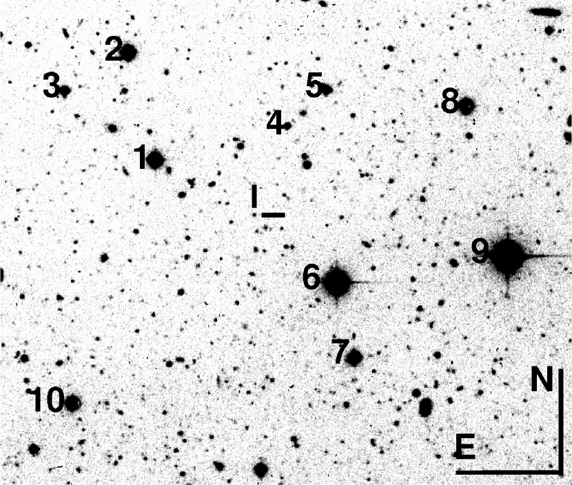
Figure 1: Reference stars in the surroundings of the GRB 021004 location (bracketed into tick marks). The depicted field of view is 4.3^′ x 4.0^′.

Table 1: Calibration stars in the GRB 021004 field, marked in Fig. 1.

	U	B	V	R
1	17.37$\pm$0.03	17.34$\pm$0.03	16.70$\pm$0.01	16.33$\pm$0.01
2	18.54$\pm$0.04	17.43$\pm$0.03	16.26$\pm$0.01	15.54$\pm$0.02
3	20.70$\pm$0.04	19.48$\pm$0.02	17.90$\pm$0.02	17.06$\pm$0.02
4	—	21.12$\pm$0.11	19.74$\pm$0.04	18.78$\pm$0.06
5	—	19.76$\pm$0.03	18.29$\pm$0.02	17.36$\pm$0.03
6	16.49$\pm$0.05	15.51$\pm$0.03	14.44$\pm$0.05	13.88$\pm$0.06
7	18.10$\pm$0.02	18.09$\pm$0.01	17.49$\pm$0.01	17.14$\pm$0.01
8	17.83$\pm$0.16	17.61$\pm$0.02	16.71$\pm$0.01	16.20$\pm$0.02
9	14.71$\pm$0.09	14.62$\pm$0.08	13.97$\pm$0.05	13.62$\pm$0.08
10	17.62$\pm$0.06	17.84$\pm$0.03	17.32$\pm$0.01	17.00$\pm$0.01
	I	J	H	K
1	15.95$\pm$0.02	15.48$\pm$0.07	15.16$\pm$0.10	14.90$\pm$0.14
2	14.90$\pm$0.03	14.06$\pm$0.03	13.47$\pm$0.03	13.36$\pm$0.05
3	16.08$\pm$0.05	15.01$\pm$0.04	14.46$\pm$0.06	14.18$\pm$0.08
4	17.83$\pm$0.06	—	—	—
5	16.46$\pm$0.03	15.41$\pm$0.06	14.72$\pm$0.06	14.44$\pm$0.10
6	13.39$\pm$0.07	12.56$\pm$0.02	12.07$\pm$0.02	11.95$\pm$0.02
7	16.79$\pm$0.03	16.33$\pm$0.13	15.84$\pm$0.16	—
8	15.70$\pm$0.03	14.96$\pm$0.04	14.43$\pm$0.05	14.61$\pm$0.11
9	13.25$\pm$0.09	12.61$\pm$0.02	12.23$\pm$0.02	12.18$\pm$0.02
10	16.64$\pm$0.02	16.20$\pm$0.11	15.75$\pm$0.14	—

2.2 Millimetre observations

The dataset is completed with observations obtained in 230 GHz and 90 GHz bands (see Table  2) at the 6-antenna Plateau de Bure Interferometer (PdB, Guilloteau et al. Guil92 (1992)). Data calibration was done with CLIC and the UV plane fitting and analysis with MAPPING, which are part of the GILDAS software package. MWC349 was used as primary flux calibrator and 0109+224 as phase calibrator.

Table 2: Millimetre observations of the GRB 021004 afterglow at PdB.

Date 2002	Frequency	Flux	Flux Error
(UT)	(GHz)	(mJy)	(mJy)
Oct 5.9844	86.293	2.47	0.29
Oct 5.9844	231.700	1.22	1.22
Oct 6.1458	115.261	1.62	1.44
Oct 6.1458	231.700	0.22	3.65
Oct 7.1438	87.717	2.57	0.56
Oct 7.1438	232.034	3.26	1.54
Oct 10.981	86.235	1.67	0.34
Oct 10.981	208.475	4.71	1.96
Oct 19.919	92.016	0.97	0.25
Oct 19.919	231.972	1.60	1.00
Nov 5.9813	97.991	0.15	0.27
Nov 5.9813	239.551	-0.33	0.71

3 Brief description of the modelling

Our starting point is the standard fireball model (see e.g. Piran Piran2005 (2005)). To account for the observed light curve brightenings, we modify the model by adding multiple energy injection episodes (see Björnsson et al. Bjor04 (2004) and in particular Jóhannesson et al. Joha05 (2005) for a detailed discussion of the expressions and formulae used). We assume that the central engine releases, essentially simultaneously, several shells with different Lorentz factors. The evolution of the fireball is then derived, as in Rhoads (Rhoa99 (1999)), from the conservation of energy and momentum. The fastest moving shell drives the initial evolution of the afterglow, but as it decelerates, the slower moving shells catch up with the shock front, producing an energy injection. Each shell collision is assumed to be instantaneous and the dynamics of the interaction is neglected, as well as any reverse shock contribution (these are expected to contribute mostly at early stages in the fireball evolution).

As in the standard fireball model, the afterglow radiation is assumed to be of synchrotron origin and the local spectrum at each point in the radiating shell is approximated by smoothly joined power law segments (similar to Granot & Sari Gran02 (2002)). Assuming that the shell is homogeneous in the co-moving frame, its thickness is obtained from the shock conditions (Blandford & McKee Blan76 (1976)) and from the conservation of swept up particles. The total flux at a given frequency and observer time is then obtained by integrating over the equal arrival time surface (Granot et al. Gran99 (1999) and references therein). The polarization light curve and position angle can be calculated adapting the model of Ghisellini & Lazzati (Ghis99 (1999)) to the fireball model (see Björnsson et al. Bjor04 (2004)).

4 Results

4.1 Multiwavelength light curves

Fig. 2 shows the light curves in the visible, NIR and millimetre bands for GRB 021004. The optical/NIR data points are plotted together with other published data (Fox et al. Fox03 (2003); Uemura et al. Uemu03 (2003); Pandey et al. Pand03 (2003); Bersier et al. Bers03 (2003); Holland et al. Holl03 (2003); Mirabal et al. Mira03 (2003); Pak et al. Pak05 (2005)) in order to show the complexity of the light curves.

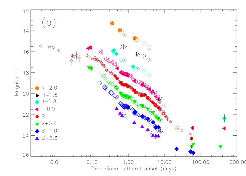
Figure 2: a) Optical and NIR light curves of GRB 021004 for the first $\sim$ 500 days after the event. The different bands have been intentionally separated for clarity. Our observations are marked with filled symbols while published data are represented with void ones (see text for references). b) Millimetre light curves for the first $\sim$ 35 days, obtained at PdB.

4.2 The optical and NIR SFD

As a starting point all the optical/NIR magnitudes are corrected for foreground Galactic extinction ($E{(B-V)}=0.06$; Schlegel et al. Sche98 (1998)). Then, we estimate the restframe extinction ($A_{V}$) and the favoured extinction law based on the afterglow optical/NIR spectral flux distribution (SFD) constructed for several epochs. The selected epochs are those for which a quasi-simultaneous wide optical/NIR coverage is available. The SFDs are clustered around 9 epochs displayed in Table 3. For each subset of photometric measurements we subtract the underlying host galaxy (see Sect. 4.4). This contribution is significant only after the first week. Finally, we fit each SFD by using a power law dimmed with different extinction laws (Pei Pei92 (1992)): Milky Way (MW), Large Magellanic Cloud (LMC) and Small Magellanic Cloud (SMC).

We obtain the best $\chi^{2}/d.o.f.$ (where d.o.f. stands for degree of freedom) with the SMC extinction law (see Table 4), as it has been previously observed for other GRB afterglows (Jensen et al. Jens01 (2001); Fynbo et al. Fynb01 (2001); Holland et al. Holl03 (2003)). For each epoch the spectral slope ($\beta$; the flux being $F_{\nu}\propto\nu^{-\beta}$) and $A_{V}$ are calculated. We can adopt the averaged SMC values for $A_{V}$ and $\beta$ since there is no evolution of the SFD on the considered time interval. The mean value inferred for the extinction and spectral index are, $\langle A_{V}\rangle=0.20\pm 0.08$, and $\langle\beta\rangle=0.5\pm 0.2$, respectively.

We note that the unextinguished SFD in the optical/NIR range might not be well represented by a perfect power law spectrum, showing some degree of intrinsic convex curvature (see the shape of the spectra in Fig. 4). Thus, the $A_{V}$ values displayed in Table 4 have to be considered a formal upper limit, likely close to the real ones. The inferred $\langle A_{V}\rangle$ is used as the starting point for correcting the intrinsic extinction of the object when applying the model.

Table 3: The GRB 021004 SFD at 9 epochs, an SMC extinction law has been assumed.

SFD #	Time since outburst	$\beta$	$A_{V}$	$\chi^{2}/d.o.f.$
	onset (days)
1	0.3609	0.43$\pm$0.18	0.17$\pm$0.04	0.8
2	0.6380	0.30$\pm$0.07	0.24$\pm$0.02	3.1
3	0.7851	0.20$\pm$0.10	0.29$\pm$0.04	1.5
4	1.4216	0.47$\pm$0.24	0.17$\pm$0.06	1.7
5	1.6304	0.82$\pm$0.14	0.08$\pm$0.06	0.3
6	1.8090	0.47$\pm$0.09	0.24$\pm$0.03	1.3
7	2.7018	0.39$\pm$0.08	0.26$\pm$0.03	0.6
8	3.6520	0.78$\pm$0.10	0.09$\pm$0.04	2.6
9	5.7388	0.47$\pm$0.20	0.25$\pm$0.06	0.4

Table 4: Mean $\chi^{2}/d.o.f.$ obtained by fitting each extinction law on the 9 available SFDs.

Extinction Law	NE	MW	LMC	SMC
$\langle\chi^{2}/d.o.f.\rangle$	11$\pm$7	11$\pm$9	3.2$\pm$1.9	2.0$\pm$1.4

4.3 Afterglow model

A number of attempts have been made to explain the nature of the bumps seen in this GRB’s light curve (Lazzati et al. Lazz02 (2002); Schaefer et al. Scha03 (2003); Nakar et al. Naka03 (2003)).

In the present work we show that the light curve can also be described by multiple energy injections, using the model of Björnsson et al. (Bjor04 (2004)). Our multiwavelength data is fitted along with other measurements reported in the literature, optical and NIR data cited in Sect. 4.1 together with X-ray data from Sako & Harrison (2002a , 2002b ) and radio data from Berger et al. (Berg02 (2002)) and Frail & Berger (Frai02 (2002)). The model only reproduces the afterglow, hence the contribution of the host galaxy has been subtracted (see Sect. 4.4).

This GRB is located at a redshift of z=2.3293 (Castro-Tirado et al. ajct05 (2005)) which shifts the Lyman-$\alpha$ break to the range of the U-band. Thus, we must consider a correction for the Lyman-$\alpha$ blanketing that appears at shorter wavelengths. We use the model described by Madau (Mada95 (1995)) at this redshift and convolve it with the Johnson U-band. This yields a reduction of the measured flux to 82% of the original one. Due to the uncertainty of this approximation we do not use the corrected U-band for fitting the model, but only for the verification of it.

From the analysis of the SFD done in the optical/NIR range (Sect. 4.2), an SMC extinction law with of $A_{V}\lesssim 0.2$ is favoured. The multiband fitting has been tested using a grid of extinctions ranging from zero to $A_{V}=0.4$ (within 2.5 sigma of the best fit value obtained from the optical/NIR SFD fitting). After several iterations we find that the best fit of the whole multi-range data set is achieved with $A_{V}\sim 0.1$.

The parameters that result from the best fit of our model are displayed in Table  5. The fitted model is characterized by an initial shock followed by 7 subsequent refreshed shocks, the last injection being the most energetic. The number of injection episodes is higher than in Björnsson et al. (Bjor04 (2004)), as a result of a more complete dataset. Two injections are needed to account for late time radio data, and one ($E_{2}$) is added to better model an optical bump at $\approx 0.35$ days. In addition, the electron energy index $p$ is a free parameter here, but was fixed in Björnsson et al. (Bjor04 (2004)).

Fig. 3 shows all the observational data along with the light curves predicted by the model for each band. Fig. 4 shows the evolution of the afterglow multiband SFD at three epochs. As predicted by the model, we observe an evolution of the peak frequency from infrared to radio as the afterglow decays. We note the excellent U-band light curve prediction (not used for the fit) once the Lyman-$\alpha$ blanketing is introduced.

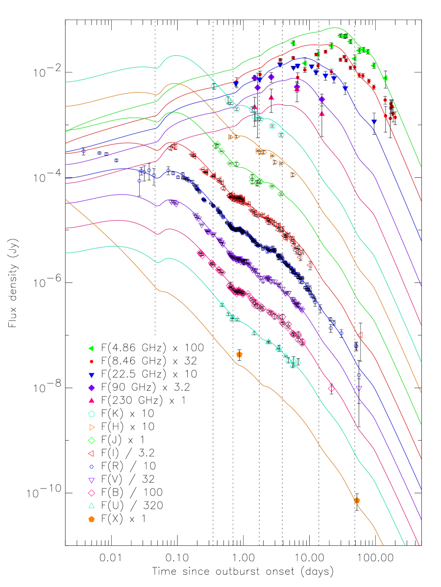
Figure 3: Multiband light curves from radio to X-rays (for the time interval 0.01 - 250 days after the burst onset) fitted with the multiple energy injection model. Seven energy injection episodes (see Table 5), indicated by vertical lines, can account for the observed behaviour. The visible and NIR observations are corrected for extinction and the U-band also for Lyman-$\alpha$ blanketing.

Table 5: The 7-injection episodes model parameters. The injection energies $E_{1}$ to $E_{7}$ are in units of $E_{0}$, the initial energy. Other model parameters are: the initial Lorentz factor $\Gamma_{0}$, the ambient density $n_{0}$, the half opening angle $\theta_{0}$, the line of sight angle $\theta_{\nu}$, the electron energy index $p$, the fraction of internal energy stored in electrons after acceleration $\epsilon_{e}$ and the fraction of internal energy stored in the form of magnetic field $\epsilon_{B}$.

Parameter	Value
$E_{0}$ (1050erg)	1.5
$E_{1}$ (0.046 days)	2.2
$E_{2}$ (0.347 days)	0.7
$E_{3}$ (0.694 days)	4.6
$E_{4}$ (1.736 days)	10.0
$E_{5}$ (3.877 days)	8.6
$E_{6}$ (13.89 days)	10.0
$E_{7}$ (48.61 days)	15.0
$\Gamma_{0}$	770
$n_{0}(cm^{-3})$	60.0
$\theta_{0}$	1$\aas@@fstack{\circ}$8
$\theta_{\nu}$	0.8$\theta_{0}$
$p$	2.2
$\epsilon_{e}$	0.35
$\epsilon_{B}$	1.7$\times$10-4

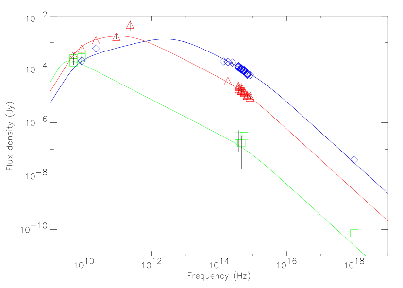
Figure 4: Evolution of the GRB 021004 afterglow SFDs at 0.8 (diamonds), 6 (triangles) and 60 days (squares) after the burst.

4.4 The host galaxy

In order to study the SFDs and constrain the model of the afterglow we need to isolate the flux produced by the afterglow from that of the underlying host galaxy. For the study of the host galaxy we use the $BVIJ$-band magnitudes measured when the contribution of the afterglow was negligible, between $\sim 62$(B) and $\sim 454$(J) days after the burst.

The fit of the host galaxy SFD is based on HyperZ (Bolzonella et al. Bolz00 (2000)). The fitting assumes Solar metallicity, a Miller & Scalo (Mill79 (1979)) initial mass function (IMF), and an SMC extinction law (Prévot et al. Prev84 (1984)). The best fit ($\chi^{2}/d.o.f.$ = 0.1) is obtained with a $\sim 15$ Myr starburst galaxy with an absolute magnitude of $M_{B}=-22.0\pm 0.3$ and an intrinsic extinction of $A_{V}=0.06\pm 0.08$ (see Fig.  5).

For the subtraction of the host galaxy colours in all the optical/NIR bands, it is necessary to predict its magnitudes in the $URHK$-bands, for which no photometric information is available. Convolving the spectra of the fitted galaxy with standard optical and infrared filters, a prediction of those magnitudes is possible (see Table 6), assuming the transformations given by Fukugita et al. (Fuku95 (1995)). The U-band must be corrected for Lyman-$\alpha$ blanketing as described in Sect. 4.3. In order to calculate the errors of the estimated magnitudes, a Monte Carlo method is used, in which the fitting of the galaxy is repeated with randomly modified input $BVIJ$ magnitudes (Gaussianly weighted) in the measured error range.

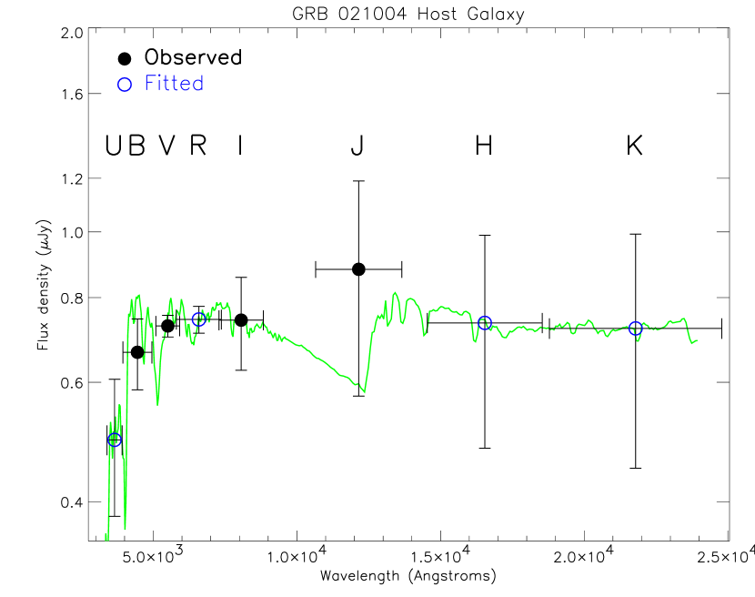
Figure 5: A fit to the photometric points of the GRB 021004 host galaxy yielding a starburst galaxy template. The H-band limit of 21.5 magnitude ($\sim 2.7\mu$ Jy) is not plotted. The filled points are our observations while the open ones are obtained from the fit of the galaxy. The flux density is represented in logarithmic scale.

Table 6: Magnitudes for the GRB 021004 host galaxy. The values marked with ^⋆ are measured values, while the rest are predictions obtained from the fitted template. The magnitudes are given in the Vega system and are not corrected for Galactic reddening.

Band	Magnitude
U	24.49 $\pm$ 0.28
B	24.65 $\pm$ 0.13⋆
V	24.45 $\pm$ 0.04⋆
R	24.21 $\pm$ 0.05
I	23.82 $\pm$ 0.17⋆
J	23.15 $\pm$ 0.38⋆
H	22.92 $\pm$ 0.31
K	22.42 $\pm$ 0.37
$\star$ Measured values.

5 Discussion

We show that the multiwavelength observations can be satisfactorily reproduced in the context of the refreshed shock model. It is capable of reproducing the ”bumpy” behaviour of the entire light curve of this event, not only the visible bands, but in a spectral range that spans from radio to X-rays. In addition, the variations in the polarization of the afterglow are naturally explained in the framework of the energy injections (Björnsson et al. Bjor04 (2004)). The number of required model parameters can be quite large, and depends on the structure of the light curve and modelling detail required.

The bumpy light curve behaviour may also be explained by the patchy shell model (Nakar et al. Naka03 (2003)), or by density variations in the surrounding medium (Lazzati et al. Lazz02 (2002)), although in the latter case, simultaneously accounting for the polarization measurements appears to be problematic. As in the refreshed shock model, the number of required parameters in these models also increases with the amount of structure in the light curve.

The afterglow model assumes an adiabatic expansion, so the proposed scenario might not be valid at very early times, when this assumption does not apply. Additionally, at early time, there can also be a strong contribution from the early reverse shock to the light curve. This might explain the excess of R-band flux observed during the first minutes that followed the burst. The very last points of our dataset for GRB  021004 may indicate a transition to a non-relativistic expansion regime. We have not included all of the relevant modifications required to capture such a transition in detail and our model results may therefore be inaccurate at very late times.

Although the X-ray observations are very limited (only two measurements), there seems to be an excess in the observed flux as compared to the model. This could be due to inverse Compton effect as seen in other GRBs (Harrison et al. Harr01 (2001), in´t Zand et al. Zand01 (2001), Castro-Tirado et al. ajct03 (2003)), an effect not considered in our modelling. The correction for the Lyman-$\alpha$ blanketing in the U-band that we introduced in Sect. 4.3 shifts the photometric points consistently with the prediction of the GRB model.

The inferred host galaxy extinction ($A_{V}$), dominant stellar age ($\sim 15$ Myr) and galaxy type (starburst) are consistent with the findings reported by Fynbo et al. (Fynb05 (2005)) for GRB 021004. The age and the extinction are also consistent with the ones derived for GRB hosts in general, being similar to young starburst galaxies present in the Hubble Deep Field sample (Christensen et al. Chri04 (2004)). However, the $B$-band absolute magnitude of the host galaxy of GRB 021004 ($M_{B}\simeq-22.0$) is brighter than the 10 hosts present in the above mentioned sample.

6 Conclusions

Due to the early detection and rapid follow-up of GRB 021004 we have had the opportunity of obtaining a very complete dataset concerning temporal range, wavelength coverage and sample density. This has allowed us to introduce important constrains on the models capable to explain the bumps present in the afterglow light curve.

In our analysis we assume several energy injection episodes to explain the light curve. A reasonable scenario includes an initial burst followed by 7 refreshed shocks. These add up to a total burst energy of 7.8x10⁵¹ ergs, that were emitted through a collimated jet with an initial half-opening angle of 1$\aas@@fstack{\circ}$8, pointing almost directly towards us.

A study of the photometric data of the host galaxy of GRB 021004 reveals a bright ($M_{B}=-22.0\pm 0.3$) starburst galaxy with low extinction ($A_{V}=0.06\pm 0.08$).

Further tests of afterglow models with this multiwavelength dataset are encouraged. Future efforts should be aimed towards obtaining multiwavelength photometry and polarimetric observations in order to be able to discriminate between the different models.

[x]cccccc Optical and NIR observations carried out for the GRB 021004 afterglow. The magnitudes are in the Vega system and not corrected for Galactic reddening.

Date UT Telescope Filter Texp (s) Mag ErMag
continued.
Date UT Telescope Filter Texp (s) Mag ErMag
2002 Oct 4.9792 2.2CAHA U 900 19.15 0.07
2002 Oct 5.0986 2.2CAHA U 900 19.59 0.08
2002 Oct 5.1785 2.2CAHA U 900 19.83 0.09
2002 Oct 5.9653 2.2CAHA U 1200 20.48 0.08
2002 Oct 6.9284 2.2CAHA U 1800 20.89 0.08
2002 Oct 7.9767 2.2CAHA U 600 21.16 0.17
2002 Oct 9.2990 1.0USNO U 5$\times$1800 21.70 0.14
2002 Oct 10.244 1.0USNO U 1800 21.73 0.25
2002 Oct 11.269 1.0USNO U 4$\times$1800 21.76 0.17

2002 Oct 5.4890 1.0USNO B 1200 20.30 0.05
2002 Oct 5.9844 2.2CAHA B 600 20.86 0.05
2002 Oct 6.0300 1.52Loiano B 1800 20.73 0.11
2002 Oct 6.9537 2.2CAHA B 1800 21.17 0.04
2002 Oct 6.9965 1.52Loiano B 2$\times$2400 21.42 0.09
2002 Oct 7.9522 2.2CAHA B 1200 21.41 0.06
2002 Oct 9.3160 1.0USNO B 5$\times$900 21.74 0.06
2002 Oct 10.115 3.5TNG B 2$\times$300 22.12 0.05
2002 Oct 11.287 1.0USNO B 4$\times$1200 22.20 0.11
2002 Oct 26.050 4.2WHT B 7$\times$300 24.28 0.13
2002 Nov 27.003 2.5INT B 10$\times$600 24.54 0.05
2002 Dec 5.762 6.0SAO B 3600 24.65 0.13

2002 Oct 4.5857 0.6MOA Blue(V) 180 16.90 0.05
2002 Oct 4.5934 0.6MOA Blue(V) 180 16.91 0.04
2002 Oct 4.6002 0.6MOA Blue(V) 180 17.01 0.03
2002 Oct 4.9896 2.2CAHA V 300 18.93 0.05
2002 Oct 5.1090 2.2CAHA V 300 19.32 0.05
2002 Oct 5.1882 2.2CAHA V 300 19.54 0.05
2002 Oct 5.4780 1.0USNO V 600 19.71 0.04
2002 Oct 5.5232 0.6MOA Blue(V) 2$\times$600 19.77 0.09
2002 Oct 5.5330 0.6MOA Blue(V) 600 19.76 0.13
2002 Oct 5.5593 0.6MOA Blue(V) 2$\times$600 19.71 0.07
2002 Oct 5.6060 0.6MOA Blue(V) 3$\times$600 19.74 0.07
2002 Oct 5.9920 2.2CAHA V 300 19.74 0.07
2002 Oct 6.0110 1.52Loiano V 1200 20.18 0.06
2002 Oct 6.1240 1.52Loiano V 900 20.15 0.31
2002 Oct 6.8650 1.52Loiano V 1800 20.52 0.13
2002 Oct 6.9410 1.52Loiano V 2$\times$1800 20.75 0.08
2002 Oct 6.9595 2.2CAHA V 600 20.55 0.05
2002 Oct 7.9668 2.2CAHA V 600 20.85 0.06
2002 Oct 9.3250 1.0USNO V 5$\times$600 21.20 0.05
2002 Oct 10.348 1.0USNO V 5$\times$600 21.60 0.08
2002 Oct 11.298 1.0USNO V 4$\times$600 21.75 0.10
2002 Nov 29.811 6.0SAO V 2250 24.43 0.17
2002 Dec 5.698 6.0SAO V 3600 24.13 0.09
2003 Sep 17.073 4.2WHT V 5$\times$900 24.45 0.04

2002 Oct 4.9965 2.2CAHA Rc 300 18.55 0.03
2002 Oct 5.1146 2.2CAHA Rc 300 18.96 0.02
2002 Oct 5.1938 2.2CAHA Rc 300 19.12 0.03
2002 Oct 5.4700 1.0USNO Rc 600 19.35 0.04
2002 Oct 5.5000 1.0USNO Rc 600 19.31 0.04
2002 Oct 5.9790 1.52Loiano Rc 1200 19.67 0.06
2002 Oct 5.9976 2.2CAHA Rc 300 19.73 0.03
2002 Oct 6.0500 1.52Loiano Rc 1200 19.87 0.06
2002 Oct 6.0620 3.5TNG Rc 2$\times$120 19.72 0.04
2002 Oct 6.8140 1.52Loiano Rc 3$\times$1800 20.20 0.08
2002 Oct 6.9687 2.2CAHA Rc 600 20.13 0.03
2002 Oct 7.9906 2.2CAHA Rc 600 20.39 0.06
2002 Oct 9.3060 1.0USNO Rc 4$\times$600 20.87 0.06
2002 Oct 10.105 3.5TNG Rc 2$\times$180 21.05 0.05
2002 Oct 10.356 1.0USNO Rc 5$\times$600 21.14 0.07
2002 Oct 11.305 1.0USNO Rc 4$\times$600 21.35 0.10
2002 Nov 29.693 6.0SAO Rc 2700 24.29 0.18

2002 Oct 4.5823 0.6MOA Red(Ic) 180 16.19 0.08
2002 Oct 4.5900 0.6MOA Red(Ic) 180 16.09 0.08
2002 Oct 4.5968 0.6MOA Red(Ic) 180 16.13 0.12
2002 Oct 5.0035 2.2CAHA Ic 600 18.09 0.08
2002 Oct 5.1215 2.2CAHA Ic 600 18.45 0.08
2002 Oct 5.2017 2.2CAHA Ic 600 18.62 0.08
2002 Oct 5.2750 1.55USNO Ic 900 18.68 0.02
2002 Oct 5.3970 1.55USNO Ic 900 18.71 0.01
2002 Oct 5.4620 1.0USNO Ic 600 18.79 0.06
2002 Oct 5.5149 0.6MOA Red(Ic) 2$\times$600 18.90 0.13
2002 Oct 5.5247 0.6MOA Red(Ic) 600 18.85 0.17
2002 Oct 5.5510 0.6MOA Red(Ic) 2$\times$600 18.61 0.11
2002 Oct 5.6067 0.6MOA Red(Ic) 3$\times$600 18.98 0.13
2002 Oct 5.9940 1.52Loiano Ic 900 19.32 0.08
2002 Oct 6.0069 2.2CAHA Ic 900 19.24 0.08
2002 Oct 6.0580 3.5TNG Ic 2$\times$120 19.22 0.04
2002 Oct 6.9120 1.52Loiano Ic 1200 19.70 0.10
2002 Oct 6.9811 2.2CAHA Ic 900 19.60 0.07
2002 Oct 8.3310 1.55USNO Ic 2$\times$900 20.09 0.02
2002 Oct 9.3120 1.0USNO Ic 4$\times$480 20.29 0.08
2002 Oct 10.363 1.0USNO Ic 5$\times$600 20.78 0.13
2002 Oct 11.313 1.0USNO Ic 4$\times$600 21.05 0.13
2002 Dec 3.000 6.0SAO Ic 2640 23.77 0.19
2003 Dec 28.888 2.5NOT Ic 14$\times$300 23.82 0.17

2002 Oct 4.8847 1.5Tirgo J 1680 16.74 0.10
2002 Oct 5.1167 1.5Tirgo J 1920 17.90 0.23
2002 Oct 5.8514 1.5Tirgo J 1680 18.06 0.39
2004 Jan 5.805 3.5CAHA J 7260 23.15 0.38

2004 Jan 7.2775 3.5CAHA H 6120 $>21.5$ —

2002 Oct 4.8622 1.5Tirgo Ks 1740 15.30 0.14
2002 Oct 5.0882 1.5Tirgo Ks 2040 15.95 0.17
2002 Oct 5.8743 1.5Tirgo Ks 1920 16.12 0.24
2002 Oct 6.0014 1.5Tirgo Ks 3480 16.71 0.21

References

- (1) Berger, E., Frail, D. A., & Kulkarni, S. R. 2002, GCN Circ. 1613.
- (2) Bersier, D., Stanek, K. Z., Winn, J. N. et al. 2003, ApJ 584, L43.
- (3) Björnsson, G., Gudmundsson, E. H., & Jóhannesson, G. 2004, ApJ 615, L77.
- (4) Blandford, R. D. & McKee, C. F., 1976, PhFl 19, 1130.
- (5) Bolzonella, M., Miralles, J.-M., & Pelló, R. 2000, A&A 363, 476.
- (6) Castro-Tirado, A. J., Gorosabel, J., Guziy, S. et al. 2003, A&A 411, L315.
- (7) Castro-Tirado, A. J., Møller, P., García-Segura, G. et al. 2005, in preparation.
- (8) Christensen, L., Hjorth, J., & Gorosabel, J., 2004, A&A 425, 913.
- (9) Fox, D.W. 2002, GCN 1564.
- (10) Fox, D.W., Yost, S., Kulkarni, S.R. et al. 2003, Nature 422, 284.
- (11) Frail, D. A., & Berger, E. 2002, GCN Circ. 1574.
- (12) Fukugita, M., Shimasaku, K., & Ichikawa, T., 1995, PASP 107, 945.
- (13) Fynbo, J.P.U., Jensen, B.L., Dall, T.H. et al., 2001, A&A 373, 796.
- (14) Fynbo, J.P.U., Gorosabel, J., Smette, A. et al., 2005, ApJ, in press.
- (15) Ghisellini, G. & Lazzati, D. 1999, MNRAS 309, L7.
- (16) Granot, J., Piran, T. & Sari, R. 1999, ApJ 513, 679.
- (17) Granot, J. & Sari, R., 2002, ApJ 568, 820.
- (18) Guilloteau S., Delannoy, J., Downes, D. et al. 1992, A&A 262, 624.
- (19) Jensen, B.L., Fynbo, J.P.U., Gorosabel, J. et al. 2001, A&A 370, 909.
- (20) Jóhannesson, G. et al. 2005, ApJ in preparation.
- (21) Harrison, F.A., Yost, S. A., Sari, R. et al. 2001, ApJ 559, 123.
- (22) Henden, A.A.,2002, GCN Circ. 1583.
- (23) Holland, S.T., Weidinger, M., Fynbo, J.P.U. et al. 2003, AJ 125, 2291.
- (24) Lazzati, D., Rossi, E., Covino, S., Ghisellini, G. & Malesani, D. 2002, A&A 396, L5.
- (25) Madau, P. 1995, ApJ 441, 18.
- (26) Miller, G. E., & Scalo, J. M. 1979, ApJS, 41, 513.
- (27) Mirabal N., Halpern, J. P., Chornock, R. et al. 2003, ApJ 595, 935.
- (28) Nakar, E., Piran, T. & Granot, J. 2003, NewA 8, 495.
- (29) Pak, S. et al. 2005, A&A, in preparation.
- (30) Pandey, S. B., Sahu, D. K., Resmi, L. et al. 2003, BASI 31, 19.
- (31) Pei, Y.C. 1992, ApJ 395, 130.
- (32) Piran, T. 2005, Rev. Mod. Phys. 76, 1143
- (33) Persson, S.E., Murphy, D.C., Krzeminski, W. et al. 1998, AJ 116, 2475.
- (34) Prévot, M. L., Lequeux, J., Prévot, L., Maurice, E., & Rocca-Volmerange, B. 1984, A&A 132, 389.
- (35) Rhoads, J. E. 1999, ApJ 525, 737.
- (36) Sako, M., & Harrison, F. A. 2002a, GCN Circ. 1624.
- (37) Sako, M., & Harrison, F. A. 2002b, GCN Circ. 1716.
- (38) Schaefer, B.E., Gerardy, C.L., Höflich, P. et al. 2003, ApJ 588, 387.
- (39) Schlegel, D.J., Finkbeiner, D.P. & Davis, M. 1998, ApJ 500, 525.
- (40) Uemura, M.,Kato, T., Ishioka, R. et al. 2003, PASJ 55, L31.
- (41) de Ugarte Postigo, A., Jelínek, M., Gorosabel, J. et al. 2005, Proceedings of the I Reunión Nacional de Astrofísica Robótica, Mazagón (Spain), in press.
- (42) in´t Zand, J. J. M., Kuiper, L., Amati, L. et al. 2001, ApJ 559, 710.