2-D models of layered protoplanetary discs:
I. The ring instability

Abstract

In this work we use the radiation hydrodynamic code TRAMP to perform a two-dimensional axially symmetric model of the layered disc. Using this model we follow the accumulation of mass in the dead zone due to the radially varying accretion rate. We found a new type of instability which causes the dead zone to split into rings. This ”ring instability” works due to the positive feedback between the thickness of the dead zone and the mass accumulation rate.

We give an analytical description of this instability, taking into account non-zero thickness of the dead zone and deviations from the Keplerian rotational velocity. The analytical model agrees reasonably well with results of numerical simulations. Finally, we speculate about the possible role of the ring instability in protoplanetary discs and in the formation of planets.

1 Introduction

The layered disc model was proposed by Gammie (1996) to account for accretion-related phenomena in T Tauri stars. He assumed that the angular momentum is transported by the magneto-rotational instability, commonly referred to as the MRI (Balbus & Hawley, 1991). However, in the outer disc (beyond $\sim 0.1$ AU) the temperature and the ionization degree is so low that the gas is not well coupled to the magnetic field and the MRI decays. There, the only parts of the disc in which the MRI can operate are the surface layers that are ionized by cosmic rays (ionization due to x-ray quanta emitted by the central star was also considered; see Glassgold, Najita & Igea 1997). Sandwiched between the active surface layers is an MRI-free, and, consequently, non-viscous area near the mid-plane of the disc, commonly referred to as the dead zone.

An interesting property of layered discs is that, in general, the accretion rate $\dot{M}$ is a function of the radius $r$. The specific form of this function depends on the mass-weighted opacity. However, $\dot{M}$ increases with $r$ if the opacity does not depend on the density and increases with the temperature not faster than $T^{2}$. This is true in the range $203$ K $<$ $T$ $<$ $2290\rho^{2/49}$ K, where the opacity is dominated by ice-free grains, and also between $167$ K and $203$ K, where the opacity drops due to the sublimation of ices as $T$ grows. At temperatures below $167$ K the opacity varies as $T^{2}$, and the accretion rate is constant as a function of $r$ (in this paper we use opacities of gas and dust mixture according to Bell & Lin 1994).

When $\dot{M}$ increases with $r$, an annulus centred at $r_{0}$ receives more mass per unit time from the outer disc $(r>r_{0})$ than that it loses to the inner disc $(r<r_{0})$. As a result, the mass accumulates in the dead zone. Eventually, at one or more locations in the dead zone the surface density becomes so large that the heat released by the accretion of the accumulated matter pushes the temperature to a level at which the collisional ionization can restore the coupling between the gas and the magnetic field. In such case a triggering event, e.g. perturbation due to the passage of the companion star, heat flux from the inner active disc or gravitational instability of the dead zone (Armitage, Livio & Pringle, 2001), could start the accretion and ”ignite” the dead zone, making at least part of it active. Consequently, the rate at which mass is accreted by the central star could increase dramatically. This mechanism was suggested by Gammie (1996) to explain the FU Ori type outbursts (Hartmann & Kenyon, 1996).

The layered disc model was further developed by Huré (2002), who noted that the non-zero thickness of the dead zone is an important factor influencing the structure of the active surface layers (this is because their structure depends on the vertical component of gravity, which in turn depends on the distance from the mid-plane). On the other hand, detailed MHD simulations of surface layers performed in a 3D shearing box approximation by Fleming & Stone (2003) showed that MRI-driven, non-axisymmetric density waves can propagate far into the dead zone. As a result, a purely HD turbulence is excited there, providing an effective viscosity.

Our original intention was to study how the evolution of the dead zone may be affected by the radiative heating from the inner active part of the disc. To that end, we performed extensive two-dimensional (axisymmetric) simulations of the evolution of layered discs, allowing for radiative energy transfer in both radial and vertical directions. Unexpectedly, we found that the dead zone is unstable in a way that has not been reported before; namely, it tends to decompose into rings. In the present paper we illustrate this ”ring” instability with numerical simulations, and we discuss it analytically, providing a physical explanation of the observed phenomena. The remaining results of our simulations will be reported in a forthcoming paper.

The outline of the present paper is as follows. In §2 we briefly describe the numerical code and we list the assumptions underlying our simulations. A layered-disc model whose dead zone decomposes into rings is presented in §3. §4 contains an analytical discussion of the ring instability. Finally, in §5 we summarize our results and discuss the effects of the ring instability in more sophisticated disc models.

2 Numerical methods

The simulations are performed with the help of the 3-D code TRAMP (Klahr et al., 1999). The equations of continuity

$$\frac{\partial\rho}{\partial t}+\nabla\cdot(\rho\mathbf{v})=0\ ,$$ (1)

momentum conservation

$$\frac{\partial\rho\mathbf{v}}{\partial t}+(\mathbf{v}\cdot\nabla)\rho\mathbf{v}=-\nabla P+\rho\nabla\Phi+\mathbf{f}_{\mathrm{cen}}+\nabla\cdot\mathbf{T}\ ,$$ (2)

and internal energy

$$c_{v}\rho\left[\frac{\partial T}{\partial t}+(\mathbf{v}\cdot\nabla)T\right]=-P\nabla\cdot\mathbf{v}+\mathbf{T}:(\nabla\mathbf{v})$$ (3)

are solved in spherical coordinates $(r,\theta,\phi)$ using an explicit operator-splitting method. $\Phi$ is here the gravitational potential, $\mathbf{f}_{\mathrm{cen}}$ is the centrifugal force, $\mathbf{T}$ is the viscous stress tensor, $\nabla\mathbf{v}$ is the rate of strain tensor composed of derivatives of velocity components, $T$ is the temperature (assumed to be the same for gas, dust and radiation), $c_{v}$ is the specific heat, and the colon denotes a double scalar product of two tensors. The self-gravity of the disc is neglected, so that

$$\Phi=\frac{GM_{\star}}{r}\ ,$$

where $M_{\star}$ is the mass of the central star. We use the equation of state of the ideal gas

$$P=\frac{k_{\mathrm{B}}T}{\mu m_{\mathrm{H}}}\rho\ ,$$ (4)

where $k_{\mathrm{B}}$ is Boltzmann constant, $\mu$ is the average molecular weight of the disc gas, and $m_{\mathrm{H}}$ is the proton mass.

The radiation transport is treated at the end of each hydrodynamic time-step by solving the equation

$$\frac{\partial E_{r}}{\partial t}=-\nabla\cdot\mathbf{F}\ ,$$ (5)

where $E_{r}=aT^{4}$ is the radiation energy density, and $\mathbf{F}$ is the radiative flux. We adopt

$$\mathbf{F}=-\frac{\lambda c}{\rho\kappa}\nabla E_{r}\ ,$$ (6)

where $\kappa$ is the Rosseland mean opacity for the gas-dust mixture (Bell & Lin, 1994), and $\lambda$ is the flux limiter used to interpolate between optically thin and optically thick cases (Levermore & Pomraning, 1981). Equations (5) and (6) are solved implicitly using an iterative SOR method. After the convergence has been achieved, the updated temperature is calculated from the updated radiation energy density. The advection routine for mass, momentum and energy is based on a second-order monotonic transport scheme originally introduced by van Leer (1977) and optimized by Kley & Hensler (1987). For more details about the numerical code we refer to Klahr et al. (1999).

The models are axially symmetric. We allow for the flow through the midplane of the disc, i.e. we do not impose a reflecting boundary condition there. Grid points are spaced logarithmically in $r$, resulting in a progressively smaller radial extent of grid cells near the centre of the disc, where their vertical extent is also progressively smaller. Thus, the shape of grid cells is more nearly regular throughout the grid.

In the inner active part of the disc, approximate initial distributions of density and temperature are obtained from analytical $\alpha$-disc models (Shakura & Sunayev, 1973) assuming a constant temperature profile in the direction perpendicular to the midplane. The outer, layered part of the disc is initiated with the analytical model of Gammie (1996). The two solutions merge at the radius $r_{\mathrm{D}Z}$, where the mid-plane temperature of the layered part reaches $1000$ K. The accretion rate of the layered part at $r_{\mathrm{D}Z}$ defines the accretion rate in the inner active part. Similarly, the surface density of the dead zone is calculated assuming continuity of the total surface density at $r_{\mathrm{D}Z}$. Initially, the surface density of the dead zone is constant in $r$. The initial rotational velocity is chosen so as to balance the gravity reduced due to the radial pressure gradient (in a thin disc the rotation is nearly Keplerian). Other components of velocity are set to zero.

At the outer edge of the disc mass is injected at every time-step at a fixed rate by the following procedure:

1. densities and temperatures are copied into the ghost zone from the adjacent active cells

2. densities in the ghost zone are normalized to the initial surface density

3. a uniform radial velocity is set across the ghost zone such that the accretion rate is the same as in the analytical model.

The angular rotational velocity at both inner and outer boundary is extrapolated using a $r^{-3/2}$ power-law. At the inner edge of the disc, and at the upper and lower boundary of the grid, a free outflow boundary condition is imposed. A constant temperature of $10$ K is maintained at the upper and lower boundary.

At each time-step the location of the dead zone is found based on two conditions that have to be fulfilled simultaneously:

1. $T<T_{\mathrm{lim}}$, where $T_{\mathrm{lim}}$ is the minimum temperature at which the coupling between the gas and the magnetic field still operates

2. $\Sigma>\Sigma_{a}$, where $\Sigma$ is the column density integrated from the surface of the disc along a line perpendicular to the midplane, and $\Sigma_{a}$ is the column density ionized by the cosmic rays.

Beyond the dead zone the viscosity coefficient is defined according to the $\alpha$-prescription of Shakura & Sunayev (1973)

$$\nu=\alpha c_{\mathrm{s}}H_{a}\ ,$$ (7)

where $\alpha$ is a dimensionless parameter, $c_{s}$ is the sound speed and $H_{a}$ is the thickness of the active layer which is determined from the vertical distribution of density for each radius at each time-step. We chose this particular form of Shakura-Sunyaev prescription because it is closer to the analytical, vertically averaged model. Within the dead zone we set $\nu=0$.

To avoid numerical problems, we introduce a density limiter: whenever the density falls below $\rho_{min}$ (which may be different for different models), it is doubled, and the temperature is adjusted so as to keep the pressure unchanged. This procedure leads to the formation of a low-density ”atmosphere” surrounding the disc. To prevent it from collapsing onto the disc, we artificially damp vertical and radial velocities in this region. However, this artificial readjustment only affects a negligible number of grid cells in the ”atmosphere”, and the overall evolution of the disc is not influenced.

3 Results of simulations

We obtained a broad sample of models with different parameters, which will be presented elsewhere. Here we describe a representative model with ”canonical” parameters $\mu=2.353$, $T_{\mathrm{lim}}=1000$ K, $\Sigma_{a}=100~{}\mathrm{g\,cm}^{-2}$ and $\alpha=0.01$. Note that at $T=1000$ K the ionization degree increases by five orders of magnitude due to ionization of potassium (Umebayashi, 1983), and the magnetic Reynolds number, which is directly proportional to the ionization degree, exceeds unity. $\Sigma=100~{}\mathrm{g\,cm}^{-2}$ is the standard stopping column density of cosmic rays (Umebayashi & Nakano, 1981), and 0.01 is a value of the viscosity parameter often adopted for protoplanetary discs (e.g. Hawley, Gammie & Balbus 1995). The simulations were performed on a grid of $256\times 45$ points in ($r$,$\theta$), with $r$ varying between 0.05 and 0.35 AU and $\theta$ varying between $-5\degr$ and $+5\degr$. The model was integrated for $124$ yr, i.e. for 600 orbits at the outer edge of the disc.

The initial model is far from thermal equilibrium, however it quickly relaxes due radiative heat diffusion. The density and mass flux across the computational domain shortly after the relaxation, at the beginning of the instability and at the end of the simulation are shown in Fig. 1: one clearly sees how the dead zone successively breaks into more and more rings.

As we have not imposed any explicit perturbations, there is a good reason to believe that the rings result from a linear instability of layered discs. The mechanism of this instability is illustrated in Fig. 2. Assume a small axially symmetric enhancement of the surface density at a radius $r_{0}$ (which, of course, must be accompanied by an increase of the dead zone thickness $H_{\mathrm{DZ}}$). Since at higher distances from the mid-plane the vertical component of gravity is stronger, the active layer (whose column density is at all times fixed by cosmic rays) must get thinner at $r_{0}$.

In the standard prescription, the viscosity coefficient is proportional to the local thickness of the active zone $H_{a}$ (this is motivated by the idea that $H_{a}$ is a natural scale that limits the maximum size of the edies of the MHD turbulence). Therefore, smaller $H_{a}$ results in a lower viscosity in the elevated part of the active layer. The accretion rate, which depends on the derivative of viscosity (see Eq. 8 below), decreases at the inner edge of the ring. This causes a bottle-neck effect in the accretion flow, and the mass accumulates in the ring. On the other hand, the higher accretion rate at the outer edge of the ring makes the ring more compact. This positive feedback between the dead zone thickness and the mass accumulation rate leads to the formation of the rings.

The rings formed in the simulation are shown in the radial profile of the surface density in Fig. 3. The accretion rate profile exhibits the described minima at the inner edges of the rings and maxima at the outer ones. The plot also shows the deviations from the Keplerian angular velocity – it can be seen that the inner edges of the rings rotate at a super-Keplerian velocity. Thus, the rings may capture and concentrate the radially drifting boulders of meter-size, preventing them from accretion onto the central star (e.g. Klahr & Lin 2000). Such concentration of solids in peaks of gas density was observed by Haghighipour & Boss (2003) and Rice et al. (2004) in the case of spiral density waves formed by the gravitational instability.

Figure 1: A detail of the computational domain around forming rings at the end of the simulation. Contours indicate density (the levels are $5\times 10^{-10}$, $10^{-9}$, $2\times 10^{-9}$, $5\times 10^{-9}$, $10^{-8}$, $2\times 10^{-8}$ and $5\times 10^{-8}$ g cm^-3), arrows denote the mass flux (for the sake of lucidity their sizes are proportional to the square root of the mass flux). The thick dash-dotted line marks the dead zone. The surface of the disc (i.e. the boundary between the disc and the atmosphere) is marked by the dashed line.

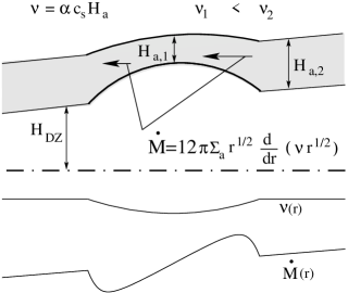
Figure 2: Upper part of the figure shows the layered disc structure with the ring-like perturbation. The higher gravitational force compresses the elevated part of the active layer, making $H_{a,1}$ smaller than the unperturbed value $H_{a,2}$. Therefore also $\nu_{1}<\nu_{2}$. The radial profiles of average viscosity and accretion rate are shown at the bottom of the figure.

Figure 3: Radial profiles of surface density $\Sigma$ (top), the accretion rate $\dot{M}$ (middle) and difference to the Keplerian angular velocity $\Omega-\Omega_{0}$ (bottom).

4 Analytical description of the ring instability

4.1 Basic assumptions and definitions

Let us consider a layered disc consisting of a dead zone with thickness $2H_{\mathrm{DZ}}$ and two active surface layers with thickness $H_{a}$ each. The surface layer accretes at a rate

$$\dot{M}=6\pi r^{1/2}\frac{\partial}{\partial r}(2\Sigma_{a}\nu r^{1/2}),$$ (8)

where $\Sigma_{a}$ is the column density of the surface layer, $\nu$ is the kinematic viscosity, and $r$ is the cylindrical radial coordinate. Equation (8) is a direct consequence of angular momentum conservation (Gammie, 1996). Assuming that the accretion energy is radiated locally, we obtain the standard formula for the effective temperature $T_{e}$

$$\frac{9}{4}\Sigma_{a}\nu\Omega^{2}=\sigma T_{e}^{4},$$ (9)

where $\sigma$ is Stefan-Boltzmann constant. In the optically thick approximation the temperature $T_{i}$ at the boundary between the dead zone and the active layer is given by the formula

$$T_{i}^{4}=\frac{3}{8}\tau T_{e}^{4}\ ,$$ (10)

where $\tau=\Sigma_{a}\kappa$ is the optical depth of the active layer, and $\kappa$ is the Rosseland mean opacity (Hubeny, 1990). In general, the opacity coefficient is a complex function of density and temperature. In a protoplanetary disc it can be approximated by a set of power laws

$$\kappa(\rho,T)=\kappa_{0}\rho^{a}T^{b}\,$$ (11)

where the constants $\kappa_{0}$, $a$ and $b$ have different values in different opacity regimes (Bell & Lin, 1994). At temperatures lower than $2290\rho^{2/49}$ K (i.e. nearly everywhere in a protoplanetary disc) $\kappa$ practically does not depend on density, so we assume $a=0$. As before, we assume that the viscosity coefficient is given by equation (7).

Let $\delta$ be the ratio of the total disc half-thickness to the active layer thickness $H_{a}$:

$$\delta\equiv\frac{H_{a}+H_{\mathrm{DZ}}}{H_{a}}\ .$$ (12)

From the equation of hydrostatic equilibrium in the direction perpendicular do the midplane of the disc we get an approximate formula

$$\frac{P_{i}}{\rho_{i}}=\Omega^{2}\delta H_{a}^{2}=c_{si}^{2}\ ,$$ (13)

where $P_{i}$, $\rho_{i}$ and $c_{\mathrm{si}}$ is, respectively, pressure, density and sound speed at the boundary between the dead zone and the active layer. Combining (13) with equations (9) and (10), and using (7) with $c_{s}=c_{\mathrm{si}}$ we get

$$T_{i}=\left[\frac{3\kappa_{0}}{8}\frac{9}{4\sigma}\frac{k_{B}}{\mu m_{\mathrm{H}}}\right]^{\frac{1}{3-b}}\Sigma_{a}^{\frac{2}{3-b}}\alpha^{\frac{1}{3-b}}\delta^{-\frac{1}{2(3-b)}}\Omega^{\frac{1}{3-b}}\ .$$ (14)

Inserting equations (9) – (14) into equation (8), we arrive at the following formula for the accretion rate in the active layer:

$$\dot{M}=\mathcal{M}r^{1/2}\frac{\partial}{\partial r}\left(\Omega^{\frac{-2+b}{3-b}}\delta^{\frac{-4+b}{2(3-b)}}r^{1/2}\right)\ ,$$ (15)

where

$$\mathcal{M}=12\pi\left[\frac{3\kappa_{0}}{8}\frac{9}{4\sigma}\right]^{\frac{1}{3-b}}\frac{k_{B}}{\mu m_{\mathrm{H}}}^{\frac{4-b}{3-b}}\Sigma_{a}^{\frac{5-b}{3-b}}\alpha^{\frac{4-b}{3-b}}\ .$$ (16)

In the following, we shall derive an equation which relates the angular rotational velocity $\Omega$ to the thickness of the disc.

Let us assume that the disc is thin ($\delta H_{a}\ll r$), and neglect the dependence of $\Omega$ on $z$ (see e.g. Urpin 1983). We may write

$$\Omega^{2}=\Omega_{0}^{2}+\frac{1}{r\rho_{m}}\frac{\partial P_{m}}{\partial r}\ ,$$ (17)

where $P_{m}=c_{\mathrm{si}}^{2}\rho_{m}$, $\rho_{m}$ and $c_{\mathrm{si}}$ are, respectively, mid-plane values of pressure, density, and sound speed. Note that because there is no heat generation in the dead zone, the mid-plane sound speed is the same as at the boundary between the dead zone and the active layer (i.e. at each $r$ the dead zone is isothermal along a line perpendicular to the midplane).

The mid-plane density $\rho_{m}$ is given by the vertical hydrostatic equilibrium

$$\rho_{m}=\rho_{i}\exp\left(\frac{\Omega^{2}H_{\mathrm{DZ}}^{2}}{2c_{\mathrm{si}}^{2}}\right)=\rho_{i}\exp\left(\frac{(\delta-1)^{2}}{2\delta}\right),$$ (18)

and for $\delta\gg 1$ we have

$$\rho_{m}=\rho_{i}\exp\left(\frac{\delta}{2}-1\right)$$ (19)

where it was assumed that the mass accumulated in dead zone is already large (i.e. $\delta\gg 1$), which allows us to neglect terms of the second order in $1/\delta$. Inserting $\rho_{\mathrm{m}}$ and $P_{\mathrm{m}}$ into equation (17) we obtain

$$\Omega^{2}=\Omega_{0}^{2}+\frac{c_{\mathrm{si}}^{2}}{2r}\frac{\partial\delta}{\partial r}+\frac{1}{r}\frac{\partial c_{\mathrm{si}}^{2}}{\partial r}+\frac{c_{\mathrm{si}}^{2}}{\rho_{i}r}\frac{\partial\rho_{i}}{\partial r}\ .$$ (20)

The sound speed $c_{\mathrm{si}}$ only weakly depends on disc thickness ($c_{\mathrm{si}}^{2}\sim\delta^{-1/5}$ for $b=0.5$). The dependence of $\rho_{i}$ on $\delta$ is even weaker ($\rho_{i}\sim\delta^{1/10}$ for $b=0.5$). Therefore, we assume that for a small perturbation of $\delta$ the last two rhs terms in equation (20), which are proportional to derivatives of $c_{\mathrm{si}}^{2}$ and $\log(\rho_{i})$, are small compared to the second rhs term, which is directly proportional to the derivative of $\delta$.

The final relation between $\Omega$ and $\delta$ is

$$\Omega^{2}=\Omega_{0}^{2}+\frac{c_{\mathrm{si}}^{2}}{2r}\frac{\partial\delta}{\partial r}\ .$$ (21)

Equations (15) and (21) will be used in the next subsections to derive the dispersion relation for the perturbations of the disc.

4.2 The linear analysis

Let us perturb $\delta$ at a radius $r_{0}$, assuming that in a small region $(r_{0}-R,r_{0}+R)$, $R\ll r$ $\delta$ consists of the unperturbed part $\delta_{0}$ (which in that region may be regarded as independent of $r$) plus a cosine term with a wavenumber $k$

$$\delta=\delta_{0}+\delta_{k}\cos(kR)\ ,$$ (22)

where $\delta_{k}$ is the amplitude of the perturbation.

According to (21), the angular velocity consists of the Keplerian part $\Omega_{0}$ and the pressure-correction $\Omega_{1}$. Neglecting terms of the second order in $\Omega_{1}$, and using equation (21) we obtain

$$\Omega^{2}=\Omega_{0}^{2}+2\Omega_{0}\Omega_{1}\quad\rightarrow\quad\Omega_{1}=\frac{c_{\mathrm{si}}^{2}}{4r\Omega_{0}}\frac{\partial\delta}{\partial r}\ .$$ (23)

The first and second derivatives of $\delta$ and $\Omega$ are

$$\begin{array}[]{ll}\frac{\partial\delta}{\partial R}=-\delta_{k}k\sin(kR)&\frac{\partial\Omega}{\partial R}=-\frac{3\Omega_{0}}{2r}-\frac{c_{\mathrm{si}}^{2}}{4r\Omega_{0}}\delta_{k}k^{2}\cos(kR)\\ \frac{\partial^{2}\delta}{\partial R^{2}}=-\delta_{k}k^{2}\cos(kR)&\frac{\partial^{2}\Omega}{\partial R^{2}}=\frac{15\Omega_{0}}{4r^{2}}+\frac{c_{\mathrm{si}}^{2}}{4r\Omega_{0}}\delta_{k}k^{3}\sin(kR)\end{array}$$ (24)

Since we only want to obtain a rough idea about the growth rate of the perturbation with a specific $k$, we may approximate $\cos(kR)$ with 1 and $\sin(kR)$ with 0. Then the disc thickness $\delta$, the angular velocity $\Omega$ and their derivatives are:

$$\delta=\delta_{0}+\delta_{k},\quad\frac{\partial\delta}{\partial R}=0,\quad\frac{\partial^{2}\delta}{\partial R^{2}}=-\delta_{k}k^{2}$$ (25)

$$\Omega=\Omega_{0},\quad\frac{\partial\Omega}{\partial R}=-\frac{3\Omega_{0}}{2r_{0}}-\frac{c_{\mathrm{si}}^{2}}{4r\Omega_{0}}\delta_{k}k^{2},\quad\frac{\partial^{2}\Omega}{\partial R^{2}}=-\frac{15\Omega_{0}}{4r_{0}}\ .$$ (26)

Due to mass accumulation, the surface density of the dead zone $\dot{\Sigma}_{\mathrm{DZ}}$ grows at a rate

$$\dot{\Sigma}_{\mathrm{DZ}}=\frac{1}{2\pi r}\frac{\partial\dot{M}}{\partial r}\ .$$ (27)

Inserting equation (15) into (27) and using approximations (25) and (26) we obtain

$$\dot{\Sigma}_{\mathrm{DZ}} = \frac{\mathcal{M}}{2\pi r_{0}}\left[\frac{3}{2}\frac{-2+b}{3-b}\Omega_{0}^{\frac{-5+2b}{3-b}}\delta^{\frac{-4+b}{2(3-b)}}\frac{\partial\Omega}{\partial R}\right.$$ (28)

$$+ \left.\frac{-4+b}{2(3-b)}r_{0}\Omega_{0}^{\frac{-2+b}{3-b}}\delta^{\frac{-10+3b}{2(3-b)}}\frac{\partial^{2}\delta}{\partial R^{2}}\right.$$

$$+ \left.\frac{-2+b}{3-b}\frac{-5+2b}{2(3-b)}r_{0}\Omega_{0}^{\frac{-8+3b}{3-b}}\delta^{\frac{-4+b}{2(3-b)}}\left(\frac{\partial\Omega}{\partial R}\right)^{2}\right.$$

$$+ \left.\frac{-2+b}{3-b}r_{0}\Omega_{0}^{\frac{-5+2b}{3-b}}\delta^{\frac{-4+b}{2(3-b)}}\frac{\partial^{2}\Omega}{\partial R^{2}}\right]$$

The linearized unperturbed part of the last equation is

$$\dot{\Sigma}_{\mathrm{DZ,0}}=\frac{3\mathcal{M}}{8\pi r_{0}^{2}}\frac{-2+b}{3-b}\frac{-9+4b}{3-b}\Omega_{0}^{\frac{-2+b}{3-b}}\delta_{0}^{\frac{-4+b}{2(3-b)}}\ ,$$ (29)

and the linearized equation which describes the evolution of surface density perturbation with wavenumber $k$ is

$$\dot{\Sigma}_{\mathrm{DZ},k} = \frac{\mathcal{M}}{2\pi r_{0}^{2}}\delta_{k}$$ (30)

$$\times \left[\frac{3}{4}\frac{-2+b}{3-b}\frac{-4+b}{2(3-b)}\frac{-9+4b}{3-b}\Omega_{0}^{\frac{-2+b}{3-b}}\delta_{0}^{\frac{-10+3b}{2(3-b)}}\right.$$

$$+ \left.\frac{3c_{\mathrm{si}}^{2}}{4}\frac{-2+b}{3-b}\frac{7-3b}{2(3-b)}\Omega_{0}^{\frac{-8+3b}{3-b}}\delta_{0}^{\frac{-4+b}{2(3-b)}}k^{2}\right.$$

$$- \left.\frac{-4+b}{2(3-b)}r_{0}^{2}\Omega_{0}^{\frac{-2+b}{3-b}}\delta_{0}^{\frac{-10+3b}{2(3-b)}}k^{2}\right]\ .$$

The surface density of the dead zone $\Sigma_{\mathrm{DZ}}$ is related to the disc thickness $\delta$ through

$$\Sigma_{\mathrm{DZ}} = 2\int_{0}^{H_{\mathrm{DZ}}}\rho(z)dz=2\int_{0}^{H_{\mathrm{DZ}}}\rho_{\mathrm{m}}\exp\left(-\frac{\Omega^{2}z^{2}}{2c_{\mathrm{si}}^{2}}\right)dz$$ (31)

$$= 2\int_{0}^{H_{\mathrm{DZ}}}\rho_{i}\exp\left(\frac{\Omega^{2}H_{\mathrm{DZ}}^{2}}{2c_{\mathrm{si}}^{2}}\right)\exp\left(-\frac{\Omega^{2}z^{2}}{2c_{\mathrm{si}}^{2}}\right)dz$$

where we used the mid-plane density given by (19). The integral can be evaluated using an error function to yield

$$\Sigma_{\mathrm{DZ}}=\frac{\sqrt{2\pi}c_{\mathrm{si}}}{\Omega}\rho_{i}\exp\left(\frac{\delta}{2}-1\right)\mathrm{erf}\left(\frac{\delta-1}{\sqrt{2\delta}}\right)\ .$$ (32)

Remembering that $\delta\gg 1$ we get

$$\Sigma_{\mathrm{DZ}}=\Sigma_{a}\sqrt{\delta}\exp\left(\frac{\delta}{2}-1\right)$$ (33)

Differentiating the last equation with respect to time leads to a formula connecting $\dot{\Sigma}_{\mathrm{DZ}}$ with $\dot{\delta}$

$$\dot{\Sigma}_{\mathrm{DZ}}=\Sigma_{a}\frac{\dot{\delta}\sqrt{\delta}}{2}\left(\frac{1}{\delta}+1\right)\exp\left(\frac{\delta}{2}-1\right)\,$$ (34)

whose unperturbed part and equation (29) can be combined into an equation

$$\dot{\delta}_{0} = \frac{3\mathcal{M}}{4\pi r_{0}^{2}\Sigma_{a}}\frac{-2+b}{3-b}\frac{-9+4b}{3-b}\Omega_{0}^{\frac{-2+b}{3-b}}\delta_{0}^{\frac{-7+2b}{2(3-b)}}$$ (35)

$$\exp\left(1-\frac{\delta_{0}}{2}\right)\left(1+\frac{1}{\delta_{0}}\right)^{-1}\ ,$$

which describes the evolution of the unperturbed disc thickness due to the accumulation of mass. Next, from equation (30), and equation (34) written for a specific wavenumber $k$ we get the dispersion relation which describes the growth rate of the perturbation with the wavenumber $k$.

$$\dot{\delta}_{k} = \frac{\mathcal{M}}{\pi r_{0}^{2}\Sigma_{a}}\exp\left(1-\frac{\delta_{0}}{2}\right)\left(1+\frac{1}{\delta_{0}}\right)^{-1}\delta_{k}$$ (36)

$$\times \left[\frac{3}{4}\frac{-2+b}{3-b}\frac{-9+4b}{3-b}\Omega_{0}^{\frac{-2+b}{3-b}}\delta_{0}^{\frac{-7+2b}{2(3-b)}}\right.$$

$$\times \left.\left(-\frac{\delta_{0}+2}{2(\delta_{0}+1)}+\frac{-4+b}{2(3-b)}\frac{1}{\delta_{0}}\right)\right.$$

$$+ \left.\frac{3c_{\mathrm{si}}^{2}}{4}\frac{-2+b}{3-b}\frac{7-3b}{2(3-b)}\Omega_{0}^{\frac{-8+3b}{3-b}}\delta_{0}^{\frac{-7+2b}{2(3-b)}}k^{2}\right.$$

$$- \left.\frac{-4+b}{2(3-b)}r_{0}^{2}\Omega_{0}^{\frac{-2+b}{3-b}}\delta_{0}^{\frac{-13+4b}{2(3-b)}}k^{2}\right]$$

The perturbation growth rate diverges at short wavelengths. This is because our simple analysis does not include any damping mechanisms. In reality, however, thin rings would diffuse due to the thermal motion of particles.

Note also that that the radial pressure scale height cannot become smaller than the vertical one. Therefore, rings with circular r-z profiles should form, which is in agreement with our numerical model (see Fig. 1).

Figure 4: Growth rates of the four inner-most rings depending on the unperturbed disc thickness $\delta_{0}$ in comparison to growth rates calculated from equation (36). Growth rates in the numerical simulation were determined by measuring $\delta$ and $\dot{\delta}$ ($\omega=\dot{\delta}/\delta$).

Fig. 4 shows growth rates of the disc thickness $\delta$ in the four inner-most rings. They are compared to the growth rates given by the dispersion relation (36). The growth rates in the analytical model are more than one order of magnitude higher. The possible explanation of this discrepancy can be that the analytical model does not allow for heat transfer from the ring into the active layer above it or for convective flows that mix the mass inside the rings. The radiative transfer in the radial direction may also be important. All those processes make the dip in the average viscosity shallower and effectively decrease the growth rate of the instability.

4.3 The influence of stellar irradiation

In this section we estimate how strongly the ring instability is affected by the radiation flux from the star. In the preceding section the stellar flux was not included self-consistently since the linear analysis presented there serves as the comparison model for the numerical simulation which does not include irradiation. On the other hand, with the irradiation included explicitly the calculations would become too complex (or just impossible) to perform.

Firstly, we estimate how important the irradiation is for the unperturbed disc. We do it by computing the change of the temperature at the boundary between the dead zone and the surface layer (from which the thickness of the surface layer and the viscosity are determined).

Stellar heating can be included in Eq. (10) in the following way

$$T_{i}^{4}=\frac{3}{8}\tau T_{e}^{4}+WT_{\star}^{4}\ ,$$ (37)

where $T_{e}$ is the effective temperature resulting solely from the viscous dissipation, $T_{\star}$ is the temperature of the stellar photosphere, and $W$ is the dilution factor which depends on stellar radius, distance from the star, and geometry of the disc (Hubeny, 1990). For a conical disc (in which the aspect ratio $H/r$ does not depend on $r$) and $r\gg R_{\star}$ we have

$$W=\frac{2}{3\pi}\left(\frac{R_{\star}}{r}\right)^{3}$$ (38)

(see e.g. Ruden & Pollack 1991).

Evaluating the rhs terms in Eq. (37) for our disc model and typical parameters of a T Tauri star ($R_{\star}=3$ R_⊙, $T_{\star}=4400$ K) we find that the first (viscous) term always dominates. More susceptible to effects of irradiation are flaring discs, in which $H/r\sim r^{\gamma}$. The flaring index $\gamma$ depends on the model, e.g. a vertically isothermal model in which the intercepted stellar flux is equal to the blackbody emission from the disc yields $\gamma=2/7$ (Chiang & Goldreich, 1997). However, even in such model the irradiation term dominates only for ($r\ga 10$ AU), where the grazing angle becomes sufficiently large.

Effects of irradiation may be more important for the ring instability itself. The inner edge of a growing ring is more strongly heated by stellar radiation, because the grazing angle $\alpha_{\mathrm{gr}}$ is larger there. As a result, the temperature and the thickness of the active layer increase locally, leading to an increased viscosity. Then, the dip in the accretion rate, which is responsible for the ring growth, becomes shallower or it may even disappear entirely.

The importance of this effect may be roughly estimated by comparing the amplitude of viscosity increase due to stellar irradiation to the amplitude of viscosity decrease due to the stronger vertical component of the gravitational force (the latter effect is explained in Fig. 2).

Let us assume a ring-like perturbation of the disc thickness with an amplitude $\delta_{k}$ and a wavelength $\lambda=2\pi/k$. Since the most unstable wavelength is $\lambda_{\mathrm{max}}\sim\delta_{0}+\delta_{k}$, let us parametrize the perturbation wavelength by the dimensionless value $l=\lambda/\lambda_{\mathrm{max}}$. The grazing angle at which the stellar radiation strikes the inner edge of the ring is

$$\alpha_{\mathrm{gr}}\sim\frac{\delta_{k}}{l(\delta_{0}+\delta_{k})}+\frac{2}{3\pi}\frac{R_{\star}}{r}\ .$$ (39)

Evaluating the dilution factor $W=\alpha_{\mathrm{gr}}(R_{\star}/r)^{2}$, inserting it into Eq. (37), and combining it with Eqs. (9), (13) and (7) we obtain the viscosity in a form

$$\nu(\delta_{k},\delta_{0},r,l) = N_{1}(r)(\delta_{0}+\delta_{k})^{\frac{-4+b}{2(3-b)}}+N_{2}(r)$$ (40)

$$\times (\delta_{0}+\delta_{k})^{-1/2}\left[\frac{\delta_{k}}{l(\delta_{0}+\delta_{k})}+N_{3}(r)\right]^{1/4}$$

where

$$N_{1}(r)=\left(\frac{3\kappa_{0}}{8}\frac{9}{4\sigma}\right)^{\frac{1}{3-b}}\alpha^{\frac{4-b}{3-b}}\left(\frac{k_{B}}{\mu m_{\mathrm{H}}}\right)^{\frac{4-b}{3-b}}\Omega^{\frac{-2+b}{3-b}}\ ,$$ (41)

$$N_{2}(r)=\frac{\alpha}{\Omega}\frac{k_{B}}{\mu m_{\mathrm{H}}}\left(\frac{R_{\star}}{r}\right)^{-1/2}T_{\star}\ ,$$ (42)

and

$$N_{3}(r)=\frac{2}{3\pi}\frac{R_{\star}}{r}\ .$$ (43)

Initially, the function $\nu(\delta_{k})$ always grows as $\delta_{k}$ increases. However, depending on the remaining parameters ($\delta_{0}$, $r$ and $l$), it may start to decrease and quickly drop below the initial value $\nu(\delta_{k}=0)$. Therefore, a very small perturbation of the disc thickness is always stabilized by the stellar irradiation, but if the amplitude of the perturbation reaches some value, the ring instability may start to work. This critical value $\delta_{k,\mathrm{crit}}$ ($\nu(\delta_{k,\mathrm{crit}})=\nu(0)$) strongly depends on $l$: it is smaller for higher $l$, where the grazing angle is smaller. The dependence on the remaining parameters ($r$ and $\delta_{0}$) for $l=3$ is shown by Fig. 5.

We see that the stabilizing effect of the irradiation may become unimportant for broad rings (large $l$), small $\delta_{0}$ (less mass accumulated in the dead zone) and/or at small radii.

Figure 5: The contours show the critical amplitude $\delta_{k,\mathrm{crit}(\delta_{0},r)}$ for which $\nu(\delta_{k,\mathrm{crit}})=\nu(0)$. Beyond their endpoints the solution becomes unphysical ($\delta_{k}>\delta_{0}$, i.e. the perturbed disk has regions with negative thickness).

5 Discussion

We described a new instability in layered accretion discs. The accretion rate in such discs is in general a function of radius. As a result, mass may accumulate in the non-viscous dead zone near the mid-plane of the disc. However, a small ring-like perturbation of the dead zone thickness leads to the deviation of the rotational velocity which results in non-uniform accumulation rate of the mass supporting growing of that ring perturbation. This ring instability may eventually lead to a decomposition of the dead zone into rings.

We observed the formation of such rings in the 2D axially symmetric radiation-hydrodynamic simulation of the layered disc. To illustrate how the instability works, we give its approximate analytical description. According to the analytical results, the narrowest rings grow most rapidly. Therefore, we may expect the formation of the radially thin rings whose radial extent will be given just by the thermal pressure of the gas. The comparison of ring sizes shows a reasonable agreement between the numerical simulation and the analytical model.

The irradiation by the central star may substantially decelerate or even stop the growth of the instability in some regions of the disc. However, broad rings are less affected, and the effects of irradiation become less important in thin discs and/or at small distances from the star. On the other hand, once the innermost ring has developed, and the flaring index $\gamma$ is not too high, the disc at larger radii is shadowed and more rings may develop there. If the disc is truncated (e.g. by the magnetosphere of the star) the shadowing effect may also be caused by its inner edge, allowing for an efficient growth of the instability.

The rings created by this instability may be important in terms of planet formation, because they can be the places where the solid particles (gravel and boulders) accumulate. It is because of the higher rotational velocity at the inner edge of the ring and the lower one at the outer edge. The drag force which makes the grains to move inwards is smaller at the inner edge of the ring and higher at the outer edge. The solid particles may merge into larger bodies (planetesimals) necessary for the formation of planets.

Massive rings are subject to a hydrodynamical instability in 3D, e.g. with respect to non-axisymmetric perturbations (Papaloizou & Pringle, 1984, 1985). This instability occurs if the rotational angular velocity decreases with radius steeper than $r^{-\sqrt{3}}$. In our simulation, this occurs for the innermost ring at a time of $\sim 280$ yr. In the non-viscous case such ring would most likely decay into so-called ”planets”, i.e. large scale vortices, as found in numerical simulations by Hawley (1987), and further investigated by Goodman, Naryan & Goldreich (1987). The fate of such a ring in 3D viscous hydro-simulations including the effects of layered accretion still have to be performed.

Our model assumes zero viscosity in the dead zone. However, there are some indications (Fleming & Stone, 2003) that even in the dead one there might be some turbulence present, induced by waves originating in the active parts of the disc. In such a case, the excess of surface density could result in a higher accretion rate in the rings, and the growth of the rings would be stopped or even they might not form at all. This issue will be addressed in a forthcoming paper.

6 Acknowledgments

This research was supported in part by the European Community’s Human Potential Programme under contract HPRN-CT-2002-00308,PLANETS. RW acknowledges financial support by the Grant Agency of the Academy of Sciences of the Czech Republic under the grants AVOZ 10030501 and B3003106. MR acknowledges the support from the grant No. 1 P03D 026 26 from the Polish Ministry of Science.

References

- Armitage et al. (2001) Armitage P. J., Livio M. and Pringle J. E., 2001, MNRAS, 324, 705
- Balbus & Hawley (1991) Balbus S. A., Hawley J. F., 1991, ApJ, 376, 214
- Bell & Lin (1994) Bell K. R., Lin D. N. C., 1994, ApJ, 477, 987
- Chiang & Goldreich (1997) Chiang E. I., Goldreich P., 1997, ApJ, 490, 368
- Fleming & Stone (2003) Fleming T., Stone J. M., 2003, ApJ, 585, 908
- Gammie (1996) Gammie C. F., 1996, ApJ, 457, 355
- Glassgold et al. (1997) Glassgold A. E., Najita J., Igea J., 1997, ApJ, 480, 344
- Goodman et al. (1987) Goodman J., Naryan R., Goldreich P., 1987, 225, 695
- Haghighipour & Boss (2003) Haghighipour N., Boss A. P., 2003, in Lunar and Planetary Science Conf., 34, 1971
- Hartmann & Kenyon (1996) Hartmann L. Kenyon S. J., 1996, Annu. Rev. Astron. Astrophys., 34, 207
- Hawley (1987) Hawley J. F., 1987, MNRAS, 225, 677
- Hawley et al. (1995) Hawley J. F., Gammie C. F., Balbus S. A., 1995, ApJ, 440, 742
- Hubeny (1990) Hubeny I., 1990, ApJ, 351, 632
- Huré (2002) Huré J.-M., 2002, PASJ, 54, 775
- Klahr et al. (1999) Klahr H. H., Henning T., Kley W., 1999, ApJ, 514, 325
- Klahr & Lin (2000) Klahr H. H., Lin D. N. C., 2000, ApJ, 554, 1095
- Kley & Hensler (1987) Kley W., Hensler G., 1987, A&A, 172, 124
- Levermore & Pomraning (1981) Levermore C. D., Pomraning G. C., 1981, ApJ, 248, 321
- Papaloizou & Pringle (1984) Papaloizou J. C. B., Pringle J. E., 1984, MNRAS, 208, 721
- Papaloizou & Pringle (1985) Papaloizou J. C. B., Pringle J. E., 1985, MNRAS, 213, 799
- Rice et al. (2004) Rice W. K. M., Lodato G., Pringle J. E., Armitage P. J., Bonnell I. A., 2004, MNRAS, 355, 543
- Ruden & Pollack (1991) Ruden S. P., Pollack J. B., 1991, ApJ, 375, 740
- Shakura & Sunayev (1973) Shakura N. I., Sunyaev R. A., 1973, A&A, 24, 337
- Umebayashi (1983) Umebayashi T., 1983, Prog. Theor. Phys., 69, 480
- Umebayashi & Nakano (1981) Umebayashi T., Nakano T., 1981, PASJ, 33, 617
- Urpin (1983) Urpin V. A., 1983, Astrophys. Space Sci., 90, 79
- van Leer (1977) van Leer B., 1977, J. Comput. Phys., 23, 276