The Spectral Evolution of Transient Anomalous X-ray Pulsar XTE J1810–197

Abstract

We present a multi-epoch spectral study of the Transient Anomalous X-ray Pulsar XTE J1810$-$197 obtained with the Newton X-Ray Multi-Mirror Mission (XMM-Newton). Four observations taken over the course of a year reveal strong spectral evolution as the source fades from outburst. The origin of this is traced to the individual decay rates of the pulsar’s spectral components. A two-temperature fit at each epoch requires that the temperatures remains nearly constant at $kT_{1}=0.25$ keV and $kT_{2}=0.67$ keV while the luminosities of these components decrease exponentially with $\tau_{1}=900$ days and $\tau_{2}=300$ days, respectively. The integrated outburst energy is $E_{1}=1.3\times 10^{42}\,d^{2}_{2.5~{}kpc}$ ergs and $E_{2}=3.9\times 10^{42}\,d^{2}_{2.5~{}kpc}$ ergs for the two spectral components, respectively. One possible interpretation of the XMM-Newton observations is that the slowly decaying cooler component is the radiation from a deep heating event that affected a large fraction of the crust, while the hotter component is powered by external surface heating at the foot-points of twisted magnetic field lines, by magnetospheric currents that are decaying more rapidly. The energy-dependent pulse profile of XTE J1810$-$197 is well modeled at all epochs by the sum of a broad pulse that dominates in the soft X-rays and a narrower one at higher energies. These profiles peak at the same phase, suggesting a concentric emission geometry on the neutron star surface. The spectral and pulse evolution together argue against the presence of a significant “power-law” contribution to the X-ray spectrum below 8 keV. The extrapolated flux is projected to return to the historic quiescent level, characterized by an even cooler blackbody spectrum, by the year 2007.

1. Introduction

The bright 5.54 s X-ray pulsar XTE J1810$-$197 is the second example of a Transient Anomalous X-ray Pulsar (TAXP) and the first one confirmed by measuring a rapid spin-down rate. All of its observed and derived physical parameters are consistent with classification as an Anomalous X-ray Pulsar (AXP), one that had an impulsive outburst sometime between 2002 November and 2003 January, when it was discovered serendipitously by Ibrahim et al. (2004) using the Rossi X-ray Timing Explorer (RXTE). Its flux was observed to be declining with an exponential time constant of $269\pm 25$ days from a maximum of $F_{X}(2-10\ {\rm keV})\approx 6\times 10^{-11}$ ergs cm^-2 s^-1. The source was then localized precisely using two Target of Opportunity (ToO) observations with the Chandra X-ray Observatory by Gotthelf et al. (2004, hereafter Paper I) and Israel et al. (2004). In comparison, archival detections by several X-ray satellites indicate a long-lived quiescent baseline flux of $F_{X}(0.5-10\ {\rm keV})\approx 7\times 10^{-13}$ ergs cm^-2 s^-1 lasting at least 13 years and possibly for 23 years prior to the outburst (Paper I). Fading of an IR source within the Chandra error circle, similar to ones associated with other AXPs, confirmed its identification with XTE J1810$-$197 (Rea et al., 2004a, b). The X-ray spectra and pulse profiles from three observations obtained with XMM-Newton during the decline of the outburst were studied by Halpern & Gotthelf (2005, hereafter Paper II). The short duty cycle of activity of XTE J1810$-$197 suggests the existence of a significant population of as-yet unrecognized, although not necessarily undetected, young neutron stars (NSs).

In this paper we present a new XMM-Newton observation of XTE J1810$-$197. This data set, combined with previous XMM-Newton observations acquired over the last year, allows us to characterize the spectral evolution of a Transient AXP. We show that the decay rates of the two fitted X-ray spectral components are distinct, and can be extrapolated in time to approach the previous quiescent spectrum. For consistency with Papers I and II, we express results in terms of a maximum distance of $d=5$ kpc to the pulsar. However, there is reason to believe that XTE J1810$-$197 is significantly closer than this, and we take into account a more realistic estimate of 2.5 kpc in our discussion of proposed physical models for the X-ray emission and outburst mechanism.

2. Observations

A fourth XMM-Newton observation of XTE J1810$-$197 was obtained on 2004 September 18. The previous three observations are described in Paper II. We use the data collected with the European Photon Imaging Camera (EPIC, Turner et al. 2003) which consist of three CCD imagers, the EPIC pn and the two EPIC MOSs, each sensitive to X-rays in the $0.1-12$ keV energy range. In the following we concentrate on data taken with the EPIC pn detector, which provided a timing resolution of 48 ms in “large window” mode, for ease of comparison with the earlier data sets. The fast readout of this instrument ensures that its spectrum is not affected by photon pileup. Data collected with the two EPIC MOS sensors used the “small window” mode and “timing” mode, providing a time resolution of 0.3 s and 1.5 ms, respectively.

Figure 1.— Period evolution of XTE J1810$-$197 using timing measurements obtained with XMM-Newton as listed in Table 1. The dashed line is a chi-square fit yielding the indicated mean value of $\dot{P}$. Error bars are $95\%$ confidence and indicate probable deviations from a constant spin-down rate.

For the new data set, we followed the reduction and analysis procedures used for the previous XMM-Newton observations of XTE J1810$-$197, as outlined in Paper II. The new observation is mostly uncontaminated by flare events and the filtered data set resulted in a total of 26.5 ks of good EPIC pn exposure time (24.4 ks live time). We checked for timing anomalies that were evident in some previous EPIC pn data sets and found none. Photon arrival times were converted to the solar system barycenter using the Chandra derived source coordinates R.A. $18^{\rm h}09^{\rm m}51.\!^{\rm s}08$, decl. $-19^{\circ}43^{\prime}51.\!^{\prime\prime}7$ (J2000.0) given in Paper I.

Figure 2.— Comparison of XMM-Newton EPIC pn spectra of XTE J1810$-$197 obtained at (a) the earliest epoch (2003 September) and (b) the latest epoch (2004 September), fitted with a two-temperature blackbody model as described in the text and specified in Table 1. Although the temperatures of the blackbody components have not changed between the two epochs, the flux of the hot component (BB2) has decayed faster than the warm one (BB1). Also shown are the residuals from the best-fit models.

2.1. Spin-down Evolution of XTE J1810$-$197

The barycentric pulse period of XTE J1810$-$197 measured at each XMM-Newton observing epoch is given in Table 1. These are derived from photons obtained with both the EPIC pn and MOS cameras, with the exception of the short 2003 October 12 observation for which only EPIC pn data of sufficient time resolution is available. The errors are the 95% confidence level determined from the $Z_{1}^{2}$ test. As shown in Figure 1, the four period measurements can be fitted to yield a mean spin-down rate of $\dot{P}=(8.1\pm 0.7)\times 10^{-12}$ s s^-1 over the year-long interval. This implies a characteristic age $\tau_{\rm c}\approx 10,800$ yr, surface magnetic field $B_{\rm s}\approx 2.1\times 10^{14}$ G, and spin-down power $\dot{E}\approx 1.9\times 10^{33}$ erg s^-1, comparable to the earlier values (Ibrahim et al., 2004, and Paper II). Deviations from a constant $\dot{P}$ are evident, however, since Ibrahim et al. (2004) fitted values in the range $(1.1-2.2)\times 10^{-11}$ s s^-1 in the first 9 months of the outburst.

As discussed in paper II (§2.2), timing glitches in AXPs can result in large increases in their period derivatives [$\Delta\dot{P}/\dot{P}\sim 1$; e.g., 1E 2259+586 Iwasawa, Koyama, & Halpern (1992); Kaspi et al. (2003) and 1RXS J170849.0–400910 Dall’Osso et al. (2003)]. Accordingly, it is possible that XTE J1810$-$197 experienced a glitch and an increase in $\dot{P}$ at the time of its outburst, and that $\dot{P}$ is now relaxing to its long-term value. But since there is no prior ephemeris for XTE J1810$-$197 in its quiescent state, we do not know if its outburst was triggered by a glitch. Alternatively, the spin-down torque could have been enhanced in the early stages of the outburst by an increase over the dipole value of the magnetic field strength at the speed-of-light cylinder (Thompson, Lyutikov, & Kulkarni, 2002), or by a particle wind and Alfvén waves (Thompson & Blaes, 1998; Harding, Contopoulos, & Kazanas, 1999), effects that are expected to decline after the first few months.

2.2. Spectral Analysis and Results

XMM-Newton observations of XTE J1810$-$197 have shown that its spectrum is equally well fitted by a power-law plus blackbody model, as commonly quoted for AXPs, or a two-temperature blackbody model. In Paper II we argued that the two-temperature model is more physically motivated, while the power-law plus blackbody model suffers from physical inconsistencies. As we shall show, the new data bolster these arguments, so we concentrate mainly on the double blackbody model in this work. Table 1 presents a summary of spectral results from all four XMM-Newton observations of XTE J1810$-$197.

Table 1XMM-Newton Spectral and Timing Results for XTE J1810$-$197

Parameter	2003 Sep 8	2003 Oct 12	2004 Mar 11	2004 Sep 18
$N_{\rm H}$ ($10^{22}$ cm-2)	$0.65\pm 0.04$	$0.65\pm 0.04$	$0.65\pm 0.04$	$0.65$ (fixed)
$kT_{1}$ (keV)	$0.26\pm 0.02$	$0.29\pm 0.04$	$0.27\pm 0.02$	$0.25\pm 0.01$
$kT_{2}$ (keV)	$0.68\pm 0.02$	$0.71\pm 0.03$	$0.70\pm 0.01$	$0.67\pm 0.01$
Area $A_{1}$ (cm2)	$1.1\times 10^{13}$	$6.6\times 10^{12}$	$6.8\times 10^{12}$	$9.1\times 10^{12}$
Area $A_{2}$ (cm2)	$6.4\times 10^{11}$	$5.1\times 10^{11}$	$2.9\times 10^{11}$	$2.1\times 10^{11}$
BB1 Flux	$4.2\times 10^{-12}$	$5.4\times 10^{-12}$	$3.5\times 10^{-12}$	$2.6\times 10^{-12}$
BB2 Flux	$3.5\times 10^{-11}$	$3.0\times 10^{-11}$	$1.8\times 10^{-11}$	$1.0\times 10^{-11}$
Total Flux	$3.93\times 10^{-11}$	$3.84\times 10^{-11}$	$2.13\times 10^{-11}$	$1.29\times 10^{-11}$
$L_{\rm BB1}$(bol) (ergs s-1)	$5.2\times 10^{34}$	$5.1\times 10^{34}$	$3.9\times 10^{34}$	$3.5\times 10^{34}$
$L_{\rm BB2}$(bol) (ergs s-1)	$1.4\times 10^{35}$	$1.3\times 10^{35}$	$7.2\times 10^{34}$	$4.2\times 10^{34}$
$\chi^{2}_{\nu}$(dof)	1.1(187)	1.1(84)	1.1(194)	1.2(188)
EPIC pn exposure (ks)	11.5	6.9	17.0	26.5
EPIC pn live time (ks)	8.1	6.2	15.8	24.4
Off-axis angle (arcmin)	0.0	8.8	0.0	0.0
Count rate (s-1)	10.6	4.8	5.8	3.4
Epoch (MJD/TDB)	52890.5642044	52924.0000320	53075.4999960	53266.4999776
Period (s)	5.539344(19)	5.53943(8)	5.539425(16)	5.539597(12)

Note. — Uncertainties in spectral parameters are 90% confidence for two interesting parameters.

As with the earlier data, the 2004 September source spectrum was accumulated in a $45^{\prime\prime}$ radius aperture which encloses $\geq 95\%$ of the energy. Background was taken from a circle of the same size displaced $2\farcm 3$ along the readout direction. The spectra were grouped into bins containing a minimum of 400 counts (including background) and fitted using the XSPEC package. For this analysis the column density is held fixed at $N_{\rm H}=6.5\times 10^{21}$ cm^-2, the value determined from previous fits, which are all consistent. The best fit to the two-temperature blackbody model yields temperatures of $kT_{1}=0.25\pm 0.01$ keV and $kT_{2}=0.67\pm 0.01$ keV with a fit statistic of $\chi^{2}_{\nu}=1.2$ for 188 degrees of freedom (Fig. 2). Each of these two temperatures, which we refer to as “warm” and “hot”, respectively, remained essentially the same, nominally to within $4\%$ of that reported for the first XMM-Newton observation (see Table 1). However, the warm and hot blackbody luminosities declined by 33% and 70%, respectively, in one year. With the temperature of the hot component remaining essentially constant, its decline in luminosity is attributable to a decrease in its emitting area, $A_{2}$. The most recent value, $A_{2}=2.1\times 10^{11}\,d_{5}^{2}$ cm², is $\approx 1\%$ of the NS surface area. In the case of the warm component, the decay in flux is modest, so that it is not yet possible to decide within the errors whether the temperature or the area is the primary variable. The most recent area measurement of the warm component, $A_{1}=9.1\times 10^{12}\,d_{5}^{2}$ cm², is $\approx 50\%$ of the NS surface area.

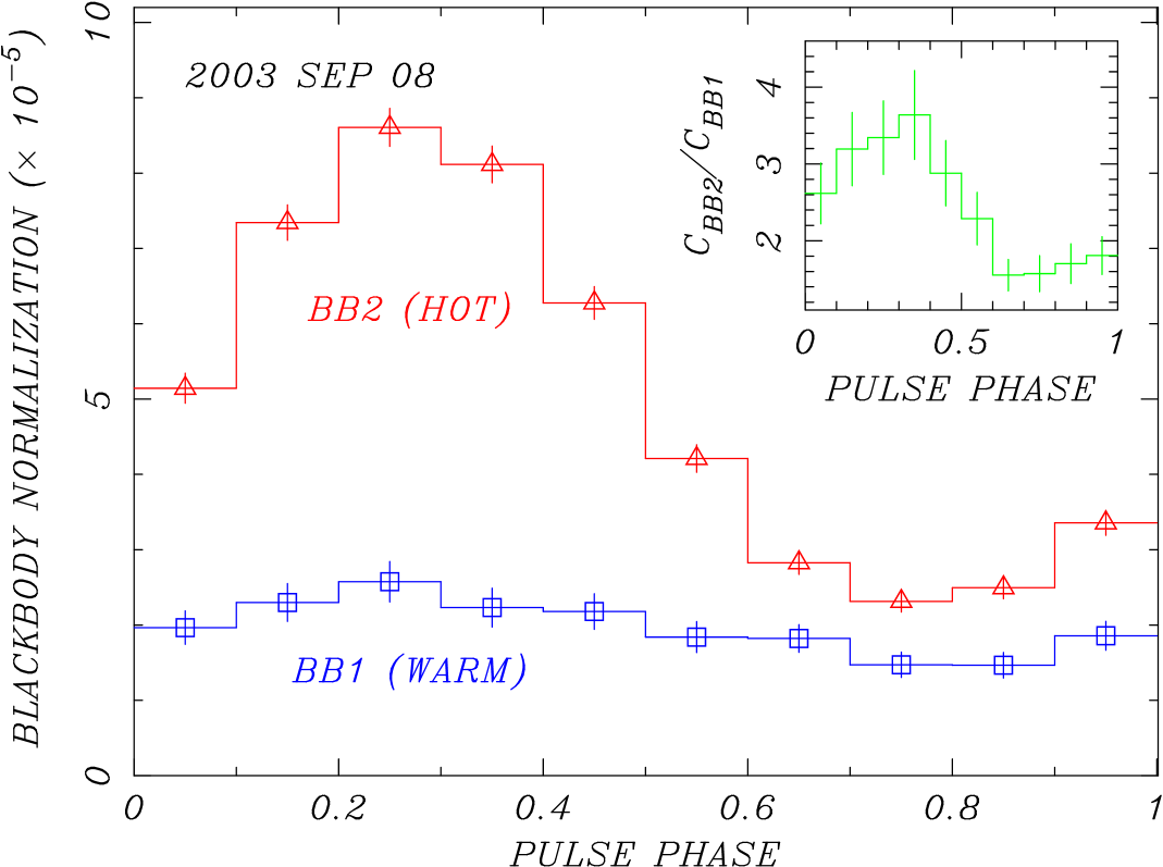
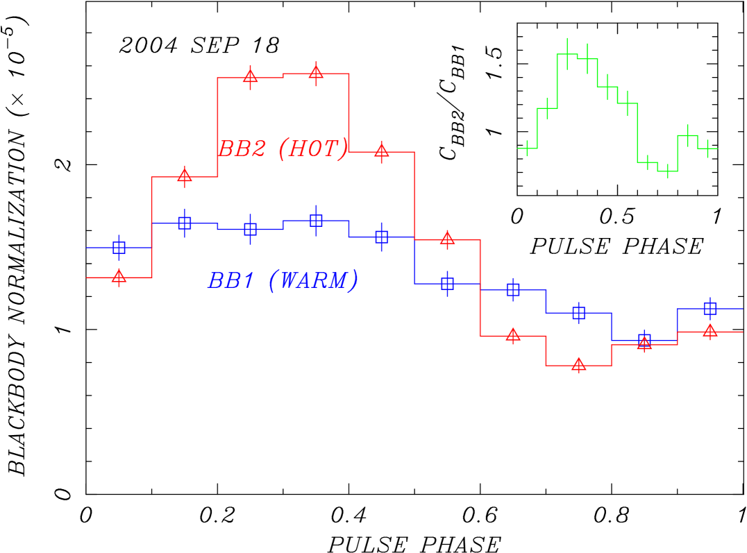
Figure 3.— Contribution of the two blackbody components as a function of rotation phase at two epochs. (Top) 2003 September. (Bottom) 2004 September. The temperatures $kT_{1}$ and $kT_{2}$ are held fixed at the values listed in Table 1, while the normalization constants are fitted. Inset: For each epoch, the ratio of blackbody normalization constants as a function of rotation phase.

Phase-resolved spectroscopy using the new XMM-Newton data set is compared here to that reported in Paper II. As before, we fit for the intensity normalization in each of 10 phase bins with the two temperatures and column density fixed at the phase-averaged value listed in Table 1. This is equivalent to determining the relative projected area of emission as a function of rotation phase. The fits are again found to be each statistically acceptable as a set, so no significant test can be made for variations in additional parameters such as the temperatures or column density. The results of the phase-resolved spectral fits are shown in Figure 3. Comparison between the data sets taken a year apart shows that the modulation with phase of each blackbody component has remained steady to within the measurement errors. The phase alignment of the two temperature components has remained the same, and the pulses peak at the same phase. This is consistent with the picture of a small, hot region surrounded by a warm, concentric annulus that occupies $\sim 1/2$ the surface area of the star. Neither component disappears at any rotation phase. In particular, if the hot component were completely eclipsed, the spectral decomposition in Figure 2 indicates that the light curves at $E>3$ keV should dip to zero; clearly they do not.

2.3. Long-term Flux Decay

With the set of XMM-Newton measurements spanning a year, a more accurate characterization of the X-ray flux decay of XTE J1810$-$197 is possible than that reported in the initial RXTE study of Ibrahim et al. (2004). The bolometric flux over time, shown in Figure 4, reveals a new and complex behavior. While the RXTE data were consistent with an exponential decay of time constant $\tau=269\pm 25$ days, the subsequent XMM-Newton measurements show that the inferred bolometric luminosity of the two spectral components are not declining at the same rate. From the data presented in Table 1 we find that the luminosity of the hotter temperature component falls exponentially with $\tau_{2}=300$ days, while the warm component decreases with $\tau_{1}=900$ days, which, although less reliably characterized, is clearly longer than $\tau_{2}$. The shorter time constant is very close to the one describing the RXTE data. Furthermore, the RXTE spectrum itself is fitted best by a single temperature blackbody of $kT=0.7$ keV (Roberts et al., 2004), without a power-law contribution, which is consistent with our interpretation of the XMM-Newton spectrum. Since RXTE is sensitive only at energies $>2$ keV where the hotter blackbody component dominates, the overall X-ray decay from the beginning of the outburst to the present appears consistent with separate exponential time constants corresponding to the two distinct thermal-spectrum components. We also note that it is not possible to fit an alternative power-law temporal decay to the hot blackbody flux; such a model would require a decay index that steepens with time.

As shown in Figure 4, we expect that the X-ray flux of XTE J1810$-$197 will return to its historic quiescent level by the year 2007. If the quiescent spectrum is to match that observed before the current outburst, then it would likely resemble the ROSAT observation of 1992 March 7. Although of relatively poor quality, the ROSAT spectrum can be reasonably well fitted with a single blackbody of $kT=0.18\pm 0.02$ keV covering $1.2\times 10^{13}\,d_{5}^{2}$ cm² and $L_{BB}({\rm bol})=1.3\times 10^{34}\,d_{5}^{2}$ ergs s^-1 (Paper I). This blackbody is significantly cooler and larger than the outburst warm component of $kT_{1}=0.25$ keV and $A_{1}=9.1\times 10^{12}\,d_{5}^{2}$ cm², so it should be present even now, although masked by the fading outburst emission. We estimate that the $kT=0.18$ keV blackbody spectrum measured with ROSAT would contribute 30% of the latest (2004 September) XMM-Newton measured flux at 0.5 keV. Therefore, we expect that such a cooler component will begin to dominate the soft X-ray spectrum in late 2006, consistent with the projection of the flux in Figure 4.

2.4. Pulse Shape Evolution

The energy-resolved folded light curves from the 2003 September 8 XMM-Newton observation (Fig. 5a) show that the pulse peak, in general, is somewhat narrower than a sinusoid, an effect that is more pronounced at higher energy. Examination of the light curves measured one year later (2004 September 18; Fig. 5d) shows a clear energy-dependent change. This is easily seen by forming the ratio of the curves taken at the two epochs, normalized by their count-weighted mean. These ratio curves, presented in Fig. 6, show changes in amplitude of up to 20%. Specifically, the pulse shape of the lower-energy light curves has evolved to a smaller amplitude, more sinusoidal profile. This change is highly significant as determined by the reduced $\chi^{2}_{\nu}$ (24 degrees-of-freedom) for the null hypothesis of a flat line (see labels on Fig. 6). In particular, the most pronounced variation is found in the 1.0–1.5 keV band with $\chi^{2}_{\nu}=6.3$ corresponding to an infinitesimal probability of the pulse shape being constant. In contrast, the pulse shape of the higher energy bins remained essentially unchanged, as evidence by their $\chi^{2}_{\nu}$ values near unity. This trend is reflected in the two intervening observations (Fig. 5c and 5d) as well.

Figure 4.— The bolometric luminosity and pulsed fraction of XTE J1810$-$197 as a function of time. (Top) The bolometric luminosity of the individual components of the two-temperature blackbody model (crosses) derived from spectral fits to XMM-Newton data with the temperatures fixed (see text). The fitted e-folding times are $\tau_{1}=900$ d and $\tau_{2}=300$ d for the warm and hot blackbody components, respectively. The fitted quantities have been extrapolated to the ($1\sigma$) quiescent range measured in Paper I (cross-hatched area). (Bottom) Pulsed fraction measurements in the $1.0-1.5$ keV energy band. The solid line represents the pulsed fraction modeled in §2.4 from the fitted decay of the blackbody components shown in the top panel.

The pulse profile must be made up of some combination of pulsed emission intrinsic to each of the two measured spectral components. In any given energy band, the changing relative contribution of the soft and hard spectral components forces the combined pulse shapes to evolve in time. One way of quantifying this change is to define the pulsed fraction $f_{p}$, the fraction of flux above the minimum in the light curve. This is found to increase smoothly with energy from 34% at less than 1 keV to $\approx 51\%$ above 5 keV at the earlier epoch (see Table 2 and Fig. 5). At the latest epoch reported herein, the pulsed fraction in the lower energy band decreased to 26% while it remained essentially unchanged at the higher energy.

The simplest hypothesis for modeling the light curve evolution is to assume that the intrinsic light curve of each spectral component is steady in time. If so, the pulsed fraction of the light curve at a given energy and epoch $f_{p}(E,t)$ can be expressed as a linear combination of two light curves of fixed pulsed fractions $f_{BB1}$ and $f_{BB2}$ weighted by the ratio of counts from the respective spectral component $N_{BB1}(E,t)$ and $N_{BB2}(E,t)$,

$$f_{p}(E,t)= {{f_{BB1}\,N_{BB1}(E,t)+f_{BB2}\,N_{BB2}(E,t)}\over{N_{BB1}(E,t)+N_{BB2}(E,t)}}$$ (1)

$$= {{f_{BB1}[1-R(E,t)]+f_{BB2}\,R(E,t)}},$$ (3)

where $R(E,t)=N_{BB2}(E,t)/[N_{BB1}(E,t)+N_{BB2}(E,t)]$ is the normalized flux ratio. This expression is only valid in the case that the minima of the two light curves coincide, as is evident for the XTE J1810$-$197 profiles. For an exponential decay of the component luminosities, the time-dependent model for the pulsed fraction is simply,

$$f_{p}(E,t)={f_{BB1}+f_{BB2}\,r(E,t_{o})\,e^{-(t-t_{o})/\tau_{d}}\over 1+r(E,t_{o})\,e^{-(t-t_{o})/\tau_{d}}},$$ (4)

where $r(E,t_{o})=N_{BB2}(E,t_{o})/N_{BB1}(E,t_{o})$ is the flux ratio at time $t_{o}$ and $\tau_{d}=(1/\tau_{2}-1/\tau_{1})^{-1}=450$ d is the differential time constant.

We can test this hypothesis directly by fitting for $f_{BB1}$ and $f_{BB2}$ using a joint least-squares fit to the set of 24 (six energy bands at four epochs) measured pulsed fractions $f_{p}(E,t)$ given in Table 2 and the ratio $R(E,t)$ for the double blackbody spectral model tabulated in Table 3. Treating the ratio $R(E,t)$ as the independent variable, the best fit yields $f_{BB2}=52\pm 3\%$ for the hotter component and $f_{BB1}=26\pm 2\%$ for the cooler one. The fit statistic is $\chi^{2}_{\nu}=1.17$ for 22 degrees-of-freedom, corresponding to a probability $\wp(\geq 1.17)=0.27$. The lower panel of Fig. 4 shows the best fit model for the decay of the the 1.0–1.5 keV pulsed fraction over time and its extrapolation to an epoch dominated by the warm spectral component. On the other hand, if we apply the blackbody plus power-law model, the corresponding values of $R(E,t)$, also listed in Table 3, are completely different and the result is $\chi^{2}_{\nu}=1.70$ for 22 degrees-of-freedom, corresponding to a probability $\wp(\geq 1.70)=0.021$, 13 times less likely relative to the double blackbody model, for the assumption of fixed intrinsic pulsed fractions.

Evidently the pulsed fraction of the hotter component is much higher than for the cooler component. This difference would account for the gradual shift from a sharper, more triangular pulse shape found at higher energies, to a rounder and more symmetric sinusoidal light curve seen at lower energies. As was hypothesized above, the decrease in pulsed fraction with time at low energies follows from the fact that the hot spectral component is decaying more rapidly than the cooler one, and so its contribution to the pulsed fraction in the low-energy bin is declining. To the extent that we are not able to discern differences greater than $\approx 4\%$, which represents the measurement uncertainty, the pulsed fractions $f_{BB1}$ and $f_{BB2}$ are individually independent of energy. However, we also cannot rule out a model in which $f_{BB1}$ itself increases with increasing energy.

Figure 5.— Energy-dependent pulse profiles of XTE J1810$-$197 obtained with the XMM-Newton EPIC pn detector. This page shows profile from epochs (a) 2003 September 8 and (b) 2003 October 12. Also shown is the best fit to the two-component model for the pulse profile (solid line) described in the text (see §2.4). The individual contibutions are plotted for the triangular component (Phase $0-1$) and the sinusoidal component (Phase $1-2$).

Fig. 5. Continued – Energy-dependent pulse profiles of XTE J1810$-$197 obtained with the XMM-Newton EPIC pn detector for (c) 2004 March 11 and (d) 2004 September 18. The epochs of phase zero are given in Table 1. Background has been subtracted. Pulsed fraction at low X-ray energies has decreased in time, while it has remained essentially unchanged at high energy.

It is useful to model the shape of the light curves of XTE J1810$-$197 in detail to further quantify their evolution. Overall, the pulse profiles suggest some linear combination of sinusoidal and triangular functions, for the soft and hard X-rays, respectively. In the following, we model the photon counts as a function of phase, $N(\phi)$, at a given energy $E$ and epoch $t$ by the two-component model,

$$N(\phi;E,t)=N_{S}(\phi;E,t)+N_{T}(\phi;E,t),$$

where

$$N_{S}(\phi;E,t)=\alpha(E,t)\,[\,1+\cos(\phi-\phi_{S})\,]+\gamma_{S}(E,t)$$

and

$$N_{T}(\phi;E,t)=\cases{\beta(E,t)\,[\,1-2|\phi-\phi_{T}|/\delta(E,t)\,]+\gamma_{T}(E,t),\cr\hfill\quad if|\phi-\phi_{T}|<\delta/2\cr\gamma_{T}(E,t),\hfill if|\phi-\phi_{T}|\geq\delta/2\cr}$$ (5)

Here, $\alpha$ is the amplitude of the pulsed signal and $\gamma_{S}$ represent the “unpulsed,” or minimum level, for the sinusoidal component, $\beta$ and $\gamma_{T}$ are the analogous parameters for the triangular component, and $\delta$ is the duty cycle (full width) of the triangular pulse.

Initial fits to the light curves indicate that the model can be constrained by fixing the triangular width $\delta$ to a single value for all observations. The same proves true for the relative phase $\phi_{S}-\phi_{T}$ between the peak fluxes of the two components. Accordingly, we used a bootstrap approach to determine these shape parameters. After finding a global fit by iteration, the triangular width is set at $\delta/2\pi=0.53$ cycles. We then determined $\phi_{S}-\phi_{T}$, which is found to be consistent with zero. Finally, the absolute phase $\phi_{S}$ at each epoch was fixed. We therefore conclude that there is no need to allow energy or time dependence for the individual component pulse shapes.

Table 2XMM-Newton Pulse Profile Fit Results for XTE J1810$-$197

Energy	2003		2004
Range	Sep 8	Oct 12	Mar 11	Sep 18
(keV)	(%)	(%)	(%)	(%)
Pulsed Fraction $f_{p}$ and (Fit Statistic $\chi^{2}_{\nu}$)
$0.5-1.0$	$34\pm 4~{}(0.9)$	$33\pm 6~{}(1.2)$	$31\pm 4~{}(0.5)$	$26\pm 3~{}(0.9)$
$1.0-1.5$	$44\pm 2~{}(0.6)$	$43\pm 3~{}(1.5)$	$40\pm 2~{}(0.8)$	$36\pm 2~{}(1.2)$
$1.5-2.0$	$48\pm 2~{}(1.5)$	$48\pm 3~{}(1.3)$	$46\pm 2~{}(1.5)$	$42\pm 2~{}(1.6)$
$2.0-3.0$	$51\pm 2~{}(1.4)$	$51\pm 3~{}(1.2)$	$50\pm 2~{}(0.9)$	$45\pm 2~{}(1.9)$
$3.0-5.0$	$54\pm 2~{}(1.2)$	$55\pm 3~{}(1.0)$	$50\pm 2~{}(1.0)$	$50\pm 2~{}(1.5)$
$5.0-8.0$	$51\pm 6~{}(2.0)$	$62\pm 5~{}(0.9)$	$48\pm 6~{}(1.5)$	$47\pm 6~{}(1.6)$
Normalized Sinusoidal Component Amplitude $\alpha$
$0.5-1.0$	$28\pm 4$	$27\pm 7$	$30\pm 4$	$22\pm 3$
$1.0-1.5$	$40\pm 2$	$37\pm 3$	$37\pm 2$	$31\pm 2$
$1.5-2.0$	$39\pm 2$	$44\pm 3$	$41\pm 2$	$39\pm 2$
$2.0-3.0$	$40\pm 2$	$39\pm 3$	$42\pm 2$	$33\pm 2$
$3.0-5.0$	$39\pm 3$	$37\pm 4$	$34\pm 3$	$33\pm 3$
$5.0-8.0$	$35\pm 8$	$34\pm 8$	$15\pm 8$	$06\pm 8$
Normalized Triangular Component Amplitude $\beta\delta/2$
$0.5-1.0$	$\phantom{0}6\pm 3$	$\phantom{0}6\pm 4$	$\phantom{0}1\pm 2$	$\phantom{0}4\pm 7$
$1.0-1.5$	$\phantom{0}5\pm 2$	$\phantom{0}6\pm 2$	$\phantom{0}4\pm 1$	$\phantom{0}4\pm 6$
$1.5-2.0$	$10\pm 2$	$\phantom{0}4\pm 2$	$\phantom{0}5\pm 1$	$\phantom{0}4\pm 6$
$2.0-3.0$	$11\pm 2$	$11\pm 3$	$\phantom{0}8\pm 1$	$11\pm 6$
$3.0-5.0$	$14\pm 2$	$18\pm 3$	$16\pm 2$	$17\pm 5$
$5.0-8.0$	$14\pm 5$	$27\pm 6$	$32\pm 5$	$40\pm 5$
Normalized Unpulsed Amplitude $\gamma$
$0.5-1.0$	$67\pm 4$	$66\pm 3$	$69\pm 3$	$74\pm 2$
$1.0-1.5$	$57\pm 2$	$56\pm 2$	$59\pm 2$	$64\pm 1$
$1.5-2.0$	$52\pm 2$	$52\pm 2$	$54\pm 2$	$58\pm 2$
$2.0-3.0$	$49\pm 2$	$49\pm 2$	$50\pm 2$	$55\pm 2$
$3.0-5.0$	$45\pm 2$	$46\pm 2$	$49\pm 2$	$50\pm 2$
$5.0-8.0$	$48\pm 5$	$38\pm 4$	$52\pm 5$	$52\pm 4$

Note. — Results of fits to the two-component sinusoidal plus triangular model for the pulse profile described in §2.4. The fixed model parameters are $\phi_{S}-\phi_{T}=0.0$, $\delta/2\pi=0.53$ cycle, and at each epoch, the absolute phase of the sinusoidal function.

Table 3Component Flux Fraction for XTE J1810$-$197

Energy	2003		2004
	——————— ———————
Range (keV)	Sep 8	Oct 12	Mar 11	Sep 18
$R(E,t)\equiv N_{BB2}/(N_{BB1}+N_{BB2})\tablenotemark{a}$
$0.5-1.0$	0.389	0.332	0.285	0.218
$1.0-1.5$	0.591	0.499	0.466	0.399
$1.5-2.0$	0.800	0.702	0.696	0.661
$2.0-3.0$	0.941	0.886	0.896	0.893
$3.0-5.0$	0.996	0.988	0.991	0.992
$5.0-8.0$	1.000	1.000	1.000	1.000
$R(E,t)\equiv N_{PL}/(N_{PL}+N_{BB})\tablenotemark{b}$
$0.5-1.0$	0.928	0.911	0.925	0.952
$1.0-1.5$	0.755	0.718	0.753	0.807
$1.5-2.0$	0.533	0.480	0.524	0.567
$2.0-3.0$	0.347	0.291	0.331	0.340
$3.0-5.0$	0.247	0.191	0.223	0.200
$5.0-8.0$	0.376	0.278	0.325	0.261

With the shape of the pulse components fixed, we fit the restricted model with just $\alpha,\beta$, and $\gamma$ ($=\gamma_{S}+\gamma_{T}$, since the $\gamma$’s are indistinguishable in this fit) as free parameters. This model fitted to all 24 individual pulse profiles yields a reduced $\chi^{2}_{\nu}$ ranging from $0.6-2.0$ with a typical value of $\chi^{2}_{\nu}=1.2$, corresponding to a probability of $\wp(\gtrsim\chi^{2}_{\nu})=0.23$ for 22 degrees-of-freedom. The best-fit model parameters, derived pulsed fractions, and fit statistic for each light curve are presented in Table 2. A clear trend is seen as the pulsed fraction decreases with time. The best-fit models are shown in Figure 5 overlaid on plots of the energy-resolved pulsed profiles for the four epochs. We checked that a single component model, either a pure sinusoidal or triangular pulse, does not adequately characterize the data based on an unacceptably large $\chi^{2}_{\nu}$ for many of the fits.

It is possible to further reduce the number of free parameters in the fit by constraining the coefficients $\alpha,\beta$, and $\gamma$ so that the phase-averaged photon count ratios $N_{S}(E,t)/N_{T}(E,t)$ are identical with the ratios derived from the two-temperature blackbody spectral fits in each energy interval at each epoch. That is, we test the hypothesis that the warm blackbody is responsible for only the sinusoidal pulse and the hot blackbody for only the triangular pulse by requiring $N_{S}(E,t)/N_{T}(E,t)=N_{BB1}(E,t)/N_{BB2}(E,t)$ at all epochs. We find that, while reasonable fits to the light curves are possible for the lower and highest energy bands, fits in the $1.5-5.0$ keV range proved unacceptable. This argues against a simple one-to-one correspondence between the spectral and the chosen light curve component decomposition. It is possible that we have not started with the correct spectral or light curve basis pairs or that the basic pulse profiles are each energy dependent. It is also possible that there may be a third, unfitted softer component associated with the quiescent flux, as seen by ROSAT (see §2.3). Continuing observation of the spectrum as the source fades should clarify the relationship between spectral and light curve components.

3. Interpretation

3.1. Spectral Evolution: Constraining Models

While the $0.5-8$ keV X-ray spectra of AXPs (including XTE J1810$-$197) clearly require a two-component fit, it is not possible to prove from spectra alone that either of two very different models, namely a power-law plus blackbody, or a two-temperature blackbody, is correct. For XTE J1810$-$197, either model yields an acceptable chi-square when fitted to the X-ray spectrum. However, in Paper II we presented physical arguments against the properties of the particular power law that results from the power-law plus blackbody fit. Unlike some rotation-powered pulsars whose spectra are fitted by hard power laws plus soft blackbodies, in AXPs the roles of these two components are reversed. For XTE J1810$-$197, most of the X-rays belonging to the $\Gamma\approx 3.7$ power-law component are lower in energy than those fitted by the blackbody (see Figure 5a of Paper II). This steep power law must turn down sharply just below the X-ray band in order not to exceed the faint, unrelated IR fluxes. As shown in Paper II, this would be difficult to achieve in a synchrotron model. And in a Comptonization model, where are the seed photons? Even if such a sharp cutoff existed at the low end of the EPIC energy band, a model in which the power-law component is due to Compton upscattering of thermal X-rays from the surface does not explain why most of the power-law photons have lower energy than the observed blackbody photons unless there is a larger source of seed photons at energies below 0.5 keV. However, such a seed source would have to be thermal emission from the neutron star. Since the two-temperature model uses a large fraction of the surface area for the $0.5-2$ keV photons, we prefer to regard the X-rays in this band as plausible seeds for, rather than as the product of, inverse Compton scattering. Supporting this assumption in the specific case of XTE J1810$-$197 are the shapes of its pulse profiles. The smooth increase in pulsed fraction with energy, and the strict phase alignment at all energies, are unnatural under the hypothesis of two different emission mechanisms and locations.

The evolving spectral shape and pulse profiles of XTE J1810$-$197 during its decline from outburst offer new and complementary evidence concerning the appropriate spectral decomposition. We find that the the pulsed fraction is declining with time at low energies, while remaining essentially constant at high energies. This fact is consistent with the changing contributions of fluxes in the two-temperature fit as the two components decline at different rates. The warm and hot components contribute significantly to the soft X-rays, whereas the hard X-rays are supplied entirely by the hot component. This is quantified in Table 3, where it is seen that the hot blackbody component accounts for 30–60% of the flux below 1.5 keV, and $>99\%$ of the flux above 3 keV at all times. Under this spectral decomposition, the pulsed fraction at energies above 3 keV is large and unchanging because one and only one spectral component is present at those energies, and it has the larger pulsed fraction of the two spectral components. In contrast, the pulsed fraction at low energies ($<1.5$ keV) is understood to decrease in time because the hot component makes only a fractional contribution to its light curve, and its fraction decreases faster than the warm spectral component, which has the intrinsically smaller pulsed fraction. This effect is also illustrated in Figure 4, where the modeled pulse fraction is compared to the data.

Figure 6.— Comparison of the XMM-Newton EPIC pn pulse profiles of XTE J1810$-$197 obtained one year apart in six energy bands. Displayed is the ratio in each band between the 2003 September 8 and 2004 September 18 profiles shown in Fig. 5, normalized by the count-weighted mean. The profiles show more systematic change at lower energies as indicated by the ratio of the amplitudes (vertical scale).

In contrast, consider how the spectral components would contribute to the various energy bands in the power-law plus blackbody spectral model. Table 3 shows that, unlike the two blackbody model, a fitted power-law component accounts for 79% of the soft ($<1.5$ keV) X-rays at all epochs, while decreasing its contribution to the hard ($>3$ keV) X-rays over time. In this model, the pulsed fraction should remain constant at low energies because only the power law is present there, while at high energies the pulsed fraction should vary because both the blackbody and the power-law components are present, in varying proportions. This spectral decomposition would drive an evolution of the pulse shapes that is opposite of what is observed. Thus, we find that the detailed evolution of the X-ray emission from XTE J1810$-$197 further supports the assumption of a purely thermal surface emission model, and leaves no evidence of a steep power law in the $0.5-8$ keV band, as is commonly fitted to individual observations of AXPs.

Our decomposition of the pulsed light curves is also consistent with the absence of modulation in the ROSAT observation of 1992 March 7, to an observed upper limit of 24% in the $0.2-2.0$  keV PSPC energy band. Since the ROSAT spectrum is fitted by an even cooler blackbody of $kT=0.18$ keV, it can be expected that the pulsed fraction in quiescence will fall below the 25% value fitted to the warm blackbody in XMM-Newton data once that component fades away.

3.2. Re-evaluation of the Distance to XTE J1810$-$197 

For consistency with Papers I and II, we have parameterized results here in terms of a distance of 5 kpc. However, this was considered an upper limit based on an H I absorption kinematic distance to the neighboring supernova remnant G11.2$-$0.3 (Green et al., 1988) and its X-ray measured column density $N_{\rm H}\sim 1.4\times 10^{22}$ cm^-2 (Vasisht et al., 1996). In comparison, the column density fitted to a power-law plus blackbody model for XTE J1810$-$197 was $N_{\rm H}=1.02\times 10^{22}$ cm^-2. Since on physical grounds we strongly prefer the double blackbody model, which requires $N_{\rm H}=0.65\times 10^{22}$ cm^-2, it seems appropriate to reduce the distance estimate to one that is more compatible with the smaller $N_{\rm H}$ value. We now assume that the distance to XTE J1810$-$197 is 2.5 kpc, and explore the consequences of this revision. The effect is to reduce the inferred X-ray luminosities and blackbody surface areas. For $d=2.5$ kpc, the surface area emitting the warm blackbody component is $A_{1}<3\times 10^{12}$ cm^-2 at all times, which is less than 1/6 the area of a neutron star. This makes it easier to understand how the pulsed fraction of the softest X-rays can be as large as $26\%$.

We can also revise the estimate of the total energy emitted in the outburst. At a distance of 2.5 kpc, the bolometric luminosity quoted in Paper II is $L_{\rm BB2}=1.5\times 10^{35}\,d_{2.5}^{2}\,e^{-(t-t_{0})/300\,{\rm days}}$ ergs s^-1 with respect to the initial time $t_{0}$ of the outburst observed by RXTE (Ibrahim et al., 2004), which corresponds to an extrapolated energy of $3.9\times 10^{42}\,d_{2.5}^{2}$ ergs. Since RXTE is only sensitive to the hotter blackbody component, we should add another contribution from the XMM-Newton measured warm component, which can be estimated as $L_{\rm BB1}=1.7\times 10^{34}\,d_{2.5}^{2}\,e^{-(t-t_{0})/900\,{\rm days}}$ ergs s^-1. The extrapolation required to integrate the contribution of the warm component is less certain than for the hot component, but it corresponds to an energy of only $1.3\times 10^{42}\,d_{2.5}^{2}$ ergs. The total estimated energy is then $5.2\times 10^{42}\,d_{2.5}^{2}$ ergs, which is comparable to the amount of heat assumed to be deposited in the crust during a deep heating event (Lyubarsky, Eichler, & Thompson, 2002), or the extra energy stored in an azimuthally twisted external magnetic field (Thompson et al., 2002). In the following section, we discuss how the observations might probe the actual mechanism of the outburst.

3.3. Heating or Cooling?

Two mechanisms have been invoked to explain the late-time “afterglow” of an outburst of a magnetar. The first involves surface heating by long-lived currents flowing on closed but azimuthally twisted external magnetic field lines, and Comptonization of the resulting surface X-ray emission by the same particles (Thompson et al., 2002). The originating event could be a sudden fracture in the crust in response to twisting of the internal magnetic field, or a plastic deformation of the crust that gradually transfers internal magnetic twist to the external field. It is thought that the major outbursts of SGRs are magnetically trapped fireballs triggered by a sudden fracture, but this is not known to apply to XTE J1810$-$197 because no bursting behavior was seen, and no prior rotational ephemeris exists to test for a glitch. In any case, the extra energy above that of a pure dipole, $\Delta E$, stored in a twisted magnetic field external to the star is,

$$\Delta E=1.4\times 10^{44}\,\Delta\phi^{2}_{\rm N-S}\,\left(B_{\rm p}\over 10^{14}\,{\rm G}\right)^{2}\,\left(R_{\rm NS}\over 10\,{\rm km}\right)^{3}\ {\rm ergs},$$ (6)

where $\Delta\phi_{\rm N-S}<1$ rad is the azimuthal twist from north to south hemisphere (Thompson et al., 2002). This is enough to account for the extrapolated $5.2\times 10^{42}\,d_{2.5}^{2}$ ergs radiated if $\Delta\phi_{\rm N-S}$ is a small fraction of a radian.

In this model, the X-ray spectrum is a combination of surface thermal emission, and Compton scattering and cyclotron resonant scattering of the thermal X-rays. Compton upscattered flux may result in power-law emission that dominates at high energies such as that reported above 10 keV for the AXP in Kes 73 (Kuiper et al., 2004). However, the flat power-law index ($\Gamma\simeq 0.94$) does not contribute to the softer spectrum, in particular below 2 keV. So we consider that the potential power-law tail in the fainter XTE J1810$-$197 may no be detectable yet. The decay timescale is determined by the rate at which power is consumed by the magnetospheric currents, which is comparable to that needed to power the observed X-ray luminosities of AXPs in general and XTE J1810$-$197 in outburst. Furthermore, it is the evolution of surface heating that basically determines the instantaneous X-ray luminosity and its decay, but more specific predictions of decay curves have not been made.

In the second picture, a deep crustal heating event, heat deposited suddenly by rearrangement of the magnetic field is gradually transferred by diffusion and radiation, and the radiated X-rays are purely thermal. While the originating event might have been a fracture of the crust as in the first scenario, an assumption that the heat is evenly distributed throughout the crust results in a particular decay curve from one-dimensional models of heat transfer (Lyubarsky et al., 2002). In this model, the heating is virtually instantaneous, within $10^{4}$ s, while it is the rate of conduction cooling that determines the observed decay curve. Lyubarsky et al. (2002) assumed a deposition of $\sim 10^{25}$ ergs cm^-3 to a depth of 500 m, which is $\leq 1\%$ of the magnetic energy density at the surface. If occurring over the entire crust, this is $\sim 1\times 10^{43}$ ergs, comparable to the total X-ray energy emitted during the decay of XTE J1810$-$197. However, Lyubarsky et al. (2002) showed that the resulting cooling luminosity would follow a $t^{-0.7}$ power law, which is rather slow compared to the observed exponential decay of the hot component of XTE J1810$-$197, while 80% of the energy should be conducted into the neutron star core rather than radiated from the surface.

It is not obvious if the behavior of XTE J1810$-$197 supports or excludes either of these models. One interesting possibility is that the slowly decaying warm component is the radiation from a deep heating event that affected a large fraction of the crust, while the hot component of the spectrum is powered by external surface heating at the foot-points of twisted magnetic field lines by magnetospheric currents that are decaying more rapidly. It is not yet clear if the flux decay of the warm component is primarily an effect of decreasing temperature or decreasing area, because the decay has so far been modest. It is possible that the decay of the warm component is consistent with a $t^{-0.7}$ power law rather than an exponential of $\tau_{1}=900$ days. Fits to $L_{BB1}$ as a function of time allows a power-law decay index in the range $-0.3$ to $-0.7$. In contrast, because of its more rapid decay, it is evident that the hotter component is declining exponentially, in area rather than in temperature. This shrinking in area might be easier to understand as a decay of the currents or a rearrangement of the magnetic field lines that are channeling the heating on the surface. But there is no good evidence yet of an inverse Compton scattered component from the particles responsible for that current, at least not at energies $<8$ keV. Perhaps the solid angle subtended by the twisted field lines in the magnetosphere is too small to scatter most of the thermal photons. Each of the models is challenged in some aspect by the observations, but each may still have some applicability. Observing the decay through to quiescence should help to clarify the situation.

3.4. Constraints on Emission and Viewing Geometry

The pulsed light curves offer an additional diagnostic of the emission and viewing geometry. If we adopt the hypothesis that virtually all of the $0.5-8$ keV flux is surface thermal emission, then the symmetry of the light curves and their strict pulse-phase alignment as a function of energy argue for a concentric geometry in which a small hot spot is surrounded by a larger, warmer region. The large observed pulsed fractions are achievable in a realistically modeled NS atmosphere that accounts for the different opacities of the normal modes of polarization in a strong magnetic field (Özel, 2001; Özel et al., 2001).

Many geometries were modeled by Özel (2001), but only total pulsed fractions were reported rather than detailed light curves. It is important to model the pulse profiles completely, since the number of peaks and their phase relationship depend in detail on the surface and viewing geometry. In addition, the relative effects of fan versus pencil beaming, as regulated by the anisotropic opacity in a strong magnetic field, allow the number of peaks in the light curve to differ from the number of hot spots on the surface. Whereas the pulsed fraction of the hot component in XTE J1810$-$197 is 53%, this is not high enough to require a single spot. It is possible that the flat interpulse region of the triangular, hard X-ray pulse is actually emission from an antipodal spot at large viewing angle. Özel et al. (2001) showed that for large magnetic fields, most of the flux would be in a broad fan beam, while Thompson et al. (2002) argue that cyclotron resonant scattering in the magnetosphere can significantly reduce this effect. Detailed physical modeling of the pulse profiles of XTE J1810$-$197 is needed before definite conclusions about the emission and viewing geometries can be drawn.

4. Conclusions and Future Work

Four sets of XMM-Newton observations of XTE J1810$-$197 spanning a year, clarify several new behaviors that might apply to other AXPs and AXP-like objects:

• a two-temperature blackbody model is arguably preferred over the standard blackbody+power law model,

• the components of the compound spectrum are decaying at rates that differ significantly, and

• the component temperatures of the blackbody emission are nearly constant, implying that the area of emission is steadily decreasing.

Several outstanding questions remain that can be addressed by continuing X-ray observations of XTE J1810$-$197 over the next few years. Will the current spectrum evolve into the prior quiescent one? Is the cool quiescent spectrum still present so that it will begin to dominate over the warm temperature component? To what degree is the quiescent emission pulsed? Why do the temperatures hardly change with time, requiring the apparent decrease in area? What is the emission geometry on the NS and what can we learn from it? Future observations will test our predictions for the flux decay and pulsed fractions and allow a better understanding of the relationship between the spectral components and the pulse profile. Ultimately, the goal of this study is to disentangle the processes of thermal and non-thermal emission to which magnetars convert their energy, during outburst and quiescence.

References

- Dall’Osso et al. (2003) Dall’Osso, S., Israel, G. L., Stella, L., Possenti, A., & Perozzi, E. 2003, ApJ, 599, 485
- Duncan & Thompson (1992) Duncan, R. C., & Thompson, C. 1992, ApJ, 392, L9
- Gotthelf et al. (2004) Gotthelf, E. V., Halpern, J. P., Buxton, M., & Bailyn, C. 2004, ApJ, 605, 368 (Paper I)
- Gotthelf et al. (1999b) Gotthelf, E. V., Vasisht, G., & Dotani, T. 1999b, ApJ, 522, L49
- Green et al. (1988) Green, D. A., Gull, S. F., Tan, S. M., & Simon, A. J. B. 1988, MNRAS, 231, 735
- Halpern & Gotthelf (2005) Halpern, J. P., & Gotthelf, E. V. 2005, ApJ, 618, 874 (Paper II)
- Harding et al. (1999) Harding, A. K., Contopoulos, I., & Kazanas, D. 1999, ApJ, 525, L125
- Ibrahim et al. (2004) Ibrahim, I. A., et al. 2004, ApJ, 609, L21
- Israel et al. (2004) Israel, G. L., et al. 2004, ApJ, 603, L97
- Iwasawa et al. (1992) Iwasawa, K., Koyama, K., & Halpern, J. 1992, PASJ, 44, 9
- Kaspi et al. (2003) Kaspi, V. M., Gavriil, F. P., Woods, P. M., Jensen, J. B., Roberts, M. S. E., & Chakrabarty, D. 2003, ApJ, 588, L93
- Kuiper et al. (2004) Kuiper, L., Hermsen, W., & Mendez, M. 2004, ApJ, 613, 1173
- Lyubarsky et al. (2002) Lyubarsky, Y., Eichler, D., & Thompson, C. 2002, ApJ, 580, L69
- Özel (2001) Özel, F. 2001, ApJ, 563, 276
- Özel et al. (2001) Özel, F., Psaltis, D., & Kaspi, V. M. 2001, ApJ, 563, 255
- Rea et al. (2004a) Rea, N., et al. 2004a, Astron. Telegram, 284, 1
- Rea et al. (2004b) ———. 2004b, A&A, 425, L5
- Roberts et al. (2004) Roberts, M. S. E., Ransom, S. M., Gavriil, F., Kaspi, V. M., Woods, P., Ibrahim, A., Markwardt, C., & Swank, J. H. 2004, in X-ray Timing 2003: Rossi and Beyond, ed. P. Kaaret, F. K. Lamb, & J. H. Swank (Melville, NY: American Institute of Physics), 306
- Thompson & Blaes (1998) Thompson, C., & Blaes, O. 1998, Phys. Rev. D, 57, 3219
- Thompson et al. (2002) Thompson, C., Lyutikov, M., & Kulkarni, S. R. 2002, ApJ, 574, 332
- Turner et al. (2003) Turner, M. J. L., Briel, U. G., Ferrando, P., Griffiths, R. G., & Villa, G. E. 2003, SPIE, 4851, 169
- Vasisht et al. (1996) Vasisht, G., Aoki, T., Dotani, T., Kulkarni, S. R., & Nagase, F. 1996, ApJ, 456, L59