Detectability of Cosmic Topology in Generalized Chaplygin Gas Models

If the spatial section of the universe is multiply connected, repeated images or patterns are expected to be detected observationally. However, due to the finite distance to the last scattering surface, such pattern repetitions could be unobservable. This raises the question of whether a given cosmic topology is detectable, depending on the values of the parameters of the cosmological model. We study how detectability is affected by the choice of the model itself for the matter-energy content of the universe, focusing our attention on the generalized Chaplygin gas (GCG) model for dark matter and dark energy unification, and investigate how the detectability of cosmic topology depends on the GCG parameters. We determine to what extent a number of topologies are detectable for the current observational bounds on these parameters. It emerges from our results that the choice of GCG as an alternative to the $\Lambda$CDM matter-energy content model has an impact on the detectability of cosmic topology.

1 Introduction

Recent advances in observational cosmology have put stringent constraints on the kind of universe we live in. Briefly, evidence points to a cosmos which is homogeneous in large scales, with spatial curvature close to zero, and where baryonic matter and radiation contribute to only about 5% of the it’s total density. The bulk of the universe’s matter-energy content seems to be composed of a pressureless component that is responsible for the observed clustering of luminous matter (accounting for almost a third of the universe’s total density), as well as a negative pressure component that drives the present phase of accelerated expansion (resposible for the remaining two thirds of the total density). Neither of these components can be directly observed and they are usually referred to as dark matter (DM) and dark energy (DE).

It has been proposed that both DE and DM may be described by a single fluid, reducing to one the unknown components of the material substratum of the universe. Among the candidates for such unifying dark matter are the Chaplygin gas, and generalizations thereof (see for example Kamenshchik et al. Kamenshchik (2001), Makler Makler (2001), and Bilić et al. Bilic (2002)). At high densities, such as those found at redshifts $z\gg 1$ or in galaxy clusters, this component behaves as DM, while at low densities (such as the average density at $z\lesssim 1$) its pressure becomes increasingly negative, explaining the current accelerated expansion of the universe. Observational data constrain the Chaplygin model’s parameter space, but does not rule it out (see, e.g., Makler et al. 2003b , Reis et al. entropy (2003), Dev et al. Dev (2004), Zhu Zhu (2004), and references therein).

In a hitherto unrelated line of research, a great deal of work has recently gone into studying the possibility that the universe may possess compact spatial sections with a non-trivial topology (for reviews, see for instance Lachièze-Rey et al. CosmTopReviews (1995), Levin CosmTopReviews3 (2002), and Rebouças & Gomero RG2004 (2004)). Many methods of detecting such topology have been proposed (see, e.g., Lehoucq et al. CitS (1998), Cornish et al. PSH (1996), and Uzan et al. CCP (1999)). The increasing accuracy of observational cosmology now makes it possible to apply these methods to existing observational data (see, e.g., Luminet et al. Poincare (2003), Cornish et al. Cornishetal03 (2004), de Oliveira-Costa et al. CMB+NonGauss (2004), and Roukema et al. Roukema (2004)).

A direct way of determining the existence of a multiply connected $3$-space section $M$ is by detecting repeated images of radiating sources, which implies that the separation between correlated pairs must be smaller than twice the radius of the observable universe, $d_{hor}$. Note however that this distance between images, being the length of the associated closed geodesic, is fixed for each nonflat topology in units of the curvature radius $a_{0}$. As a consequence, many possible topologies may be undetectable by pattern repetition, given the nearly flatness of the universe favored by current observations (see, e.g., Tegmark et al. SDSSWMAP (2004)). Thus, the ratio $\chi_{hor}=d_{hor}/a_{0}$, which depends on the cosmological model and its associated parameters, is crucial to determine the detectability of cosmic topology.

The extent to which a nontrivial topology may or may not be detected for the current bounds on the cosmological parameters is studied in Gomero et al. (2001a , 2001b ), Mota et al. (Mota03 (2003)), Weeks (NEWweeks (2003)), and Weeks et al. (NEWweeks2 (2003)). These studies have concentrated on cases where the matter-energy content is modeled within the $\Lambda$CDM framework, investigating the dependence of the detectability of the topology on the cosmological density parameters $\Omega_{m}$ and $\Omega_{\Lambda}$. Here we shall address a different question: to what extent is the detectability of the topology modified when different background cosmological models are considered? To this end, we shall focus our attention on low curvature nonflat universes whose dark-matter-energy content is dominated by the generalized Chaplygin Gas (GCG). We determine which topologies from a large family of spherical manifolds and some small-volume hyperbolic manifolds are either potentially detectable or undetectable, taking into account the current observational bounds on the GCG model. We also study the dependence of detectability on the model parameters, and in particular on the steepness of the equation of state, $\alpha$, and show that detectability becomes more likely as $\alpha$ decreases.

This paper is organized as follows. In the next section we discuss some fundamental results on the detectability of cosmic topology and provide a short review of GCG-dominated cosmological models. These two strands are brought together in section (3), which deals with our analytical and numerical results regarding the detectability of cosmic topology in the GCG case. Finally, we sum up our results and indicate points for future research in section (4).

2 Preliminaries

Most cosmologists agree that the universe is close to being spatially homogeneous and isotropic at large scales. In a general relativistic context, such a space-time is described by a $4$-manifold $\mathcal{M}$, which is decomposed into $\mathcal{M}=\mathbb{R}\times M$, and is endowed with a Robertson-Walker metric

$$ds^{2}=-dt^{2}+a^{2}(t)\left[d\chi^{2}+f^{2}(\chi)(d\theta^{2}+\sin^{2}\theta d\phi^{2})\right]\;,$$ (1)

where $a(t)$ is the scale factor and $f(\chi)=\chi\,$, $\sin\chi$, or $\sinh\chi$, depending on the sign of the curvature (respectively $k=0,1,$ or $-1$). For each of these three cases the spatial section $M$ is usually taken to be a simply-connected manifold, either euclidian $\mathbb{E}^{3}$ ($k=0$), spherical $\mathbb{S}^{3}$ ($k=1$), or hyperbolic $\mathbb{H}^{3}$ ($k=-1$). However, since geometry does not dictate topology, the $3$-space $M$ may as well be any one of a number of (multiply connected) quotient manifolds $M=\widetilde{M}/\Gamma$, where $\Gamma$ is a discrete and fixed point-free group of isometries of the covering space $\widetilde{M}=(\mathbb{E}^{3},\mathbb{S}^{3},\mathbb{H}^{3})$. The action of $\Gamma$ tessellates $\widetilde{M}$ into identical domains which are copies of what is known as the fundamental polyhedron. Hence, a point $x$ (or source) within the fundamental polyhedron can be connected to every other point in its orbit in the covering space $gx|_{g\in\Gamma}$ (i.e., its images), by a space-like geodesic, which is closed by the associated isometry. The immediate observational consequence of this is that the sky may (potentially) show multiple images of radiating sources. The closed geodesics are the projection onto $M$ of the (light-like) geodesics followed by photons emitted by the source. By observing repeated images or patterns, we are directly detecting isometries in $\Gamma$, with which we might reconstruct $M$ and thus determine the topology of the universe.

A closed geodesic that passes through $x$ in a multiply connected manifold $M$ is a segment of a geodesic in the covering space $\widetilde{M}$ that joins $x$ to one of its images. Since any such pair of points is by definition related by an isometry $g\in\Gamma$, the length of the closed geodesic associated to any fixed isometry $g$ passing through $x$ is given by the corresponding distance function $\delta_{g}(x)\equiv d(x,gx)\,$. The injectivity radius at $x$ is then defined as

$$r_{inj}(x)\equiv\frac{1}{2}\min_{g\in\Gamma,\,g\neq I}\,\{\,\delta_{g}(x)\,\}\;.$$ (2)

where $I$ is the identity of $\Gamma$. From (2) clearly the injectivity radius is the radius of the smallest sphere centered at $x$ and ‘inscribable’ in the fundamental polyhedron. Thus, any sphere with radius $r<r_{inj}(x)$ and centered at $x$ lies inside a fundamental polyhedron of $M$ based on $x$.

One can also define the global injectivity radius (simply denoted by $r_{inj}$), which is the radius of the smallest “inscribable” sphere centered at any point in $M$, or the minimum value of $r_{inj}(x)$

$$r_{inj}\equiv\min_{x\in M}\{\,r_{inj}(x)\,\}\;.$$ (3)

Due to the finite age of the universe, it is generally not possible to observe the entire covering space. For any given observational survey up to a maximum redshift $z_{obs}$, the survey depth $\chi(z_{obs},\Omega_{i0})$ in a nonflat universe can be expressed, in units of the curvature radius $a_{0}=H_{0}/\sqrt{|1-\Omega_{0}|}$, as a function of the (present time) density parameters $\Omega_{i0}=\rho_{i0}/\rho_{\mathrm{crit}}$, as

$$\chi(z_{obs},\Omega_{i0})=\frac{d_{hor}}{a_{0}}=\sqrt{|1-\Omega_{0}|}\int_{0}^{z_{obs}}\frac{H_{0}}{H(z,\Omega_{i0})}dz\;,$$ (4)

where $H(z,\Omega_{i0})$ is the Hubble parameter at redshift $z$.

Now, for a given $\chi(z_{obs},\Omega_{i0})$ (or simply $\chi_{obs}$) a topology is undetectable by an observer at a point $x$ if $\chi_{obs}<r_{inj}(x)$. In this case there are no multiple images (or pattern repetitions) in the survey. On the other hand, when $\chi_{obs}>r_{inj}(x)$, then the topology is detectable in principle for an observer at $x$. However, since we do not know a priori our position in the universe, it is more suitable for our purposes here to use a criterium valid at any $x$, stated in terms of the global injectiviy radius $r_{inj}$, which is a lower bound for $r_{inj}(x)$. The undetectability condition then is that the topology of $M$ is undetectable by any observer if $r_{inj}>\chi_{obs}$. Reciprocally, the condition $\chi_{obs}>r_{inj}$ ensures detectability in principle for at least some observers. In globally homogeneous manifolds, the distance function $d(x,gx)$ for any given isometry $g$ is constant, which means $r_{inj}(x)\equiv r_{inj}$. Therefore, if the topology is potentially detectable (or conversely, undetectable) by an observer at $x$, it is likewise potentially detectable (conversely undetectable) by any other observer at any other point in the $3$-space $M$.

We shall focus exclusively on the detectability of spherical and hyperbolic manifolds. These manifolds are rigid, which implies that geometrical quantities are topological invariants and therefore the lengths of the closed geodesics are fixed in units of the curvature radius $a_{0}$. We can therefore compare the injectivity radius $r_{inj}$ of each manifold with the survey depth $\chi_{obs}$ as a function of the matter-energy content model parameters.

The spherical $3$-manifolds are of the form $M=\mathbb{S}^{3}/\Gamma$, where $\Gamma$ is a finite subgroup of $SO(4)$ acting freely on the $3$-sphere. These manifolds were originally classified by Threlfall and Seifert (ThrelfallSeifert (1932)), and are also discussed by Wolf (Wolf (1984)) (for a description in the context of cosmic topology see Ellis Ellis71 (1971)). This classification consists essentially in the enumeration of all finite groups $\Gamma\subset SO(4)$, and then grouping all ensuing manifolds in classes. In a recent paper, Gausmann et al. (GLLUW (2001)) recast the classification in terms of single action, double action, and linked action manifolds. In table 1 we list the orientable single action manifolds together with the labels often used to refer to them, as well as the order of the covering groups $\Gamma$ and the corresponding injectivity radii. All single action manifolds are globally homogeneous, and thus the same detectability condition holds for all observers in the manifold.

Table 1: Single action spherical manifolds along with the order of the covering groups and the injectivity radii.

Name & Symbol	Order of $\Gamma$	Injectivity Radius
Cyclic $Z_{n}$	$n$	$\pi/n$
Binary dihedral $D^{*}_{m}$	$4m$	$\pi/2m$
Binary tetrahedral $T^{*}$	24	$\pi/6$
Binary octahedral $O^{*}$	48	$\pi/8$
Binary icosahedral $I^{*}$	120	$\pi/10$

Closed orientable hyperbolic $3$-manifolds can be constructed and studied with the publicly available SnapPea software package (Weeks SnapPea (1999)). Each compact hyperbolic manifold is constructed from a non-compact cusped manifold through a so-called Dehn surgery, which is a formal procedure identified by two coprime integers called winding numbers $(n_{1},n_{2})$. SnapPea names these manifolds according to the original cusped manifold and the winding numbers. So, for example, the smallest volume hyperbolic manifold known (the Weeks’ manifold) is labeled as m$003(-3,1)$, where m$003$ is the seed cusped manifold and $(-3,1)$ are the winding numbers. Hodgson and Weeks (HodgsonWeeks (1994)) have compiled a census containing $11031$ orientable closed hyperbolic 3-manifolds ordered by increasing volume. In table 2 we present the seven smallest manifolds from this census, with their respective volumes and injectivity radii $r_{inj}$.

Table 2: First seven manifolds in the Hodgson-Weeks census of closed hyperbolic manifolds, with corresponding volumes and injectivity radii.

Manifold	Volume	Injectivity Radius
m003(-3,1)	0.943	0.292
m003(-2,3)	0.981	0.289
m007(3,1)	1.015	0.416
m003(-4,3)	1.264	0.287
m004(6,1)	1.284	0.240
m004(1,2)	1.398	0.183
m009(4,1)	1.414	0.397

It is clear from the equation (4) that, since the integral is finite, as $\Omega_{0}\rightarrow 1$ more and more nonflat topologies become undetectable. To gain a more quantitative understanding of the issue of detectability, however, one must first specify the equations of state of the component densities. Therefore, the choice of model for the matter-energy content of the universe has, as we shall discuss below, important consequences for the possible detection of cosmic topology. In the present work we study the detectability of cosmic topology in a universe dominated by the GCG, which we now briefly review.

As mentioned in the introduction, the dynamics of the universe seems to be dominated by two components which are not directly observable: a pressureless DM component and a DE component with negative pressure. DM is detected by its local clustering, through dynamical measurements, such as galaxy rotation curves, velocity dispersion and $X$-ray emission by gas in clusters, and also by gravitational lensing. The observed abundance of light elements together with primordial nucleosynthesis calculations show that baryons can account for only about 15% of this clustered component (see, e.g., Bertone et al. DMreviews (2004)). On the other hand, the presence of DE is evidenced by its effects on very large scales. It seems to power the accelerated expansion discovered in type Ia supernovae (SNIa) data (see, e.g., Perlmutter et al. PerlmutterSNIa (1998), Riess et al. Riess (1998), and Tonry et al. tonry03 (2003)) and to significantly contribute to the global curvature — providing around two thirds of the density needed to explain the near flatness inferred from the cosmic microwave background radiation (CMBR) data.

Since the evidence for DM and DE involves observations at different scales and epochs, one may wonder if they could be distinct manifestations of the same component, dubbed unifying dark matter, or UDM (see, e.g., Makler et al. 2003a ). We will assume that the UDM may be modeled by a perfect fluid energy-momentum tensor whose only independent components are $p$ and $\rho$. The UDM equation of state must be such as to allow for a decelerating and non-relativistic phase in the past, followed by the present accelerated phase. Recall that the acceleration is given by $\ddot{a}=-4\pi G(\rho+3p)/3$. Thus, for the decelerating and accelerating phases to happen sequentially the UDM must be nearly pressureless at higher densities, with $|p|\ll\rho$, and also exert a large ($p\sim-\rho$) negative pressure at lower densities. A simple example of an equation of state satisfying this condition is that of the GCG (see Makler Makler (2001), Bilić et al. Bilic (2002), and Bento et al. BentoGCG (2002)), and is given by an inverse power law

$$p_{\mathrm{Ch}}=-\frac{M^{4(\alpha+1)}}{\rho_{\mathrm{Ch}}^{\alpha}}\;,$$ (5)

where $M$ is positive and has dimension of mass and $\alpha$ is an adimensional real number.

Consider now the background geometry of a universe dominated by the GCG. In this case, the energy conservation equation can be easily solved, giving the energy density of the GCG in terms of the scale factor,

$$\rho_{\mathrm{Ch}}=\rho_{\mathrm{Ch}0}\left[(1-A)\left(\frac{a_{0}}{a}\right)^{3(\alpha+1)}+A\right]^{1/(\alpha+1)},$$ (6)

where $A=(M^{4}/\rho_{\mathrm{Ch}0})^{(\alpha+1)}$. We must impose $\alpha>-1$ for the accelerated epoch to occur after the decelerated phase. We also require $0<A<1$ so that $\rho_{\mathrm{Ch}}$ is well defined at all times. Under these circumnstances, at earlier times when $a/a_{0}\ll 1$, we have $\rho_{\mathrm{Ch}0}\propto a^{-3}$ and the fluid behaves as DM. For later times, $a/a_{0}\gg 1$, and we have $p_{\mathrm{Ch}0}=-\rho_{\mathrm{Ch}0}=-M^{4}=const.$ as in the cosmological constant case. Thus, this equation of state interpolates between DM and DE while the average energy density of the universe changes, as expected from the previous discussion. It includes as special cases the standard Chaplygin gas for $\alpha=1$, and the $\Lambda$CDM model for $\alpha=0$.

We proceed now to study the interplay between the detectability of cosmic topology and the GCG parameters $A$ and $\alpha$.

3 Detectability of topology in GCG cosmology

The key point for a systematic and quantitative study of the detectability of the topology of the (nonflat) spatial section $M$ is the comparison between the injectivity radius of each manifold in units of the curvature radius $r_{inj}^{M}$ (a topological invariant) with the survey depth $\chi_{obs}$. As was pointed out in the previous section, the manifold’s topology is detectable in principle for a survey of depth $\chi_{obs}$ if the matter-energy content parameters are such that $\chi_{obs}\geq r_{inj}^{M}$. Likewise, if $\chi_{obs}<r_{inj}^{M}$ then the topology is undetectable by any pattern repetition method. Most of the work done so far focused on the $\Lambda$CDM model (see, e.g., Mota et al. Mota03 (2003)), but here we extend this approach to GCG models.

For the $\Lambda$CDM case (equivalent to $\alpha=0$ in the GCG model) the detectability conditions can be restated in terms of contour curves in the $\Omega_{m}-\,\Omega_{\Lambda}$ parametric plane. For each manifold $M$ and a given fixed redshift $z_{obs}$ we can define the contour curve $\chi(\Omega_{m},\Omega_{\Lambda},z_{obs})=r_{inj}^{M}$. This curve lies in either the positive or negative curvature semiplanes ($\Omega_{0}<1$ and $\Omega_{0}>1$ respectively), depending on whether the manifold is spherical or hyperbolic. The contour curve divides its semiplane in a region where the topology is undetectable ($\chi_{obs}<r_{inj}^{M}$), and a region where the topology is detectable in principle ($\chi_{obs}\geq r_{inj}^{M}$). Therefore, given this curve, it is possible to determine the (un)detectability of any given nonflat manifold for a range of density parameters.

In a previous work (Mota et al. Mota03 (2003)) it was shown that this contour curve can be approximated in two complementary ways by the tangent and secant lines, which respectively overestimate and underestimate detectability. It was further shown that the numerical results from both methods are in good agreement with each other for the bounds on density values obtained by Spergel et al. (WMAP-Spergel-et-al (2003)), which means they are good approximations for the contour curve. Finally, it was also shown that in the limit $z\rightarrow\infty$, the secant line can be obtained analytically. This last result is of particular interest, because it allows to study the detectability of topology not only for individual manifolds, but also for whole classes of manifolds.

While in the $\Lambda$CDM case the detectability was determined by two parameters, in the case of the GCG three parameters must be taken into account, $\Omega_{\mathrm{Ch}0}=\rho_{\mathrm{Ch}0}/\rho_{crit}$, $\,A$, and $\alpha$ (with the baryonic density $\Omega_{b0}$ kept fixed). To make the analysis simpler and comparisons easier, we introduce the new variables

$$\bar{\Omega}_{\Lambda 0} = \Omega_{\mathrm{Ch}0}\,A\;,$$

$$\bar{\Omega}_{m0} = \Omega_{\mathrm{Ch}0}\,(1-A)\;,$$ (7)

such that $\Omega_{\mathrm{Ch}0}=\bar{\Omega}_{m0}+\bar{\Omega}_{\Lambda 0}$. Notice that with this definition, for $\alpha=0$, $\bar{\Omega}_{m0}$ corresponds to a matter density parameter and $\bar{\Omega}_{\Lambda 0}$ corresponds to a cosmological constant parameter (see eq. 8 bellow).

With the definitions (3) the redshift-distance relation (4) becomes

$$\chi_{obs} =\sqrt{|1-\Omega_{0}|}\times$$

$$\int_{0}^{z}dx \left\{\Omega_{\mathrm{Ch}}+\Omega_{b0}(1+x)^{3}+(1-\Omega_{0})(1+x)^{2}\right\}^{-\frac{1}{2}},$$ (8)

where

$$\Omega_{\mathrm{Ch}}=\Omega_{\mathrm{Ch}0}\left[\frac{\bar{\Omega}_{\Lambda 0}}{\Omega_{\mathrm{Ch}0}}+\frac{\bar{\Omega}_{m0}}{\Omega_{\mathrm{Ch}0}}(1+x)^{3(1+\alpha)}\right]^{\frac{1}{1+\alpha}}$$ (9)

and $\Omega_{0}=\Omega_{\mathrm{Ch}0}+\Omega_{b0}$.

In the analytical computations that follow, we shall omit the baryon fraction. The role of $\Omega_{b0}$ will be discussed later in conjunction with the numerical computations. Thus, for a fixed $z_{obs}$ the only free parameters left are $\alpha$, $\bar{\Omega}_{m0}$, and $\bar{\Omega}_{\Lambda 0}$. For each value of $\alpha$ we can then define a parametric plane $\bar{\Omega}_{m0}-\bar{\Omega}_{\Lambda 0}$, which is very similar to the $\Omega_{m0}-\Omega_{\Lambda 0}$ plane discussed above. Unfortunately, it is not possible to analytically integrate equation (8) for a generic value of $\alpha$. Instead, we first show that $\chi_{obs}$ is a monotonically decreasing function of $\alpha$ for $\alpha\in(-1,\infty)$, and then obtain analytical expressions for the contour curves for the limiting cases $\alpha=-1$ and $\alpha\rightarrow\infty$, with $z_{obs}\rightarrow\infty$. This sets upper and lower bounds on the values $\chi_{obs}$ can take in equation (8), and guarantees that $\chi_{obs}$ will interpolate monotonically between these bounds for the intermediate values of $\alpha$.

Let us first show the monotonicity of $\chi_{obs}$ with respect to $\alpha$. Consider the term $\Omega_{\mathrm{Ch}}$ given by expression (9), with $x\geq 0$ and $\bar{\Omega}_{\Lambda 0}\neq 0$. Defining $u=(1+x)^{3(1+\alpha)}\geq 1$, a straightforward calculation shows that

$$\frac{\partial^{2}\;\Omega_{\mathrm{Ch}}}{\partial\;u\;\partial\;\alpha}=\frac{\bar{\Omega}_{m0}}{\Omega_{\mathrm{Ch}0}}\log\left[\frac{u}{\frac{\bar{\Omega}_{\Lambda}}{\Omega_{\mathrm{Ch}0}}+\frac{\bar{\Omega}_{m}}{\Omega_{\mathrm{Ch}0}}u}\right]\geq 0\;.$$ (10)

The derivative $\partial\;\Omega_{\mathrm{Ch}}/\partial\;\alpha$ is therefore an increasing function of $u$. But for $u=1$, clearly $\partial\;\Omega_{\mathrm{Ch}}/\partial\;\alpha=0$. Hence, $\partial\;\Omega_{\mathrm{Ch}}/\partial\;\alpha>0$ for any $u>1$, and $\Omega_{\mathrm{Ch}}$ is an increasing function of $\alpha.$ Thus, from (8) we have that $\chi_{obs}$ is a decreasing function of $\alpha$. As a result, the detectability of a given topology then becomes less likely as $\alpha$ increases, for fixed $\bar{\Omega}_{m}$ and $\bar{\Omega_{\Lambda}}$.

We shall now obtain analytical expressions for the contour curves in the extreme cases $\alpha=-1$ and $\alpha=\infty$ (with $\Omega_{b0}=0$). In both cases we take the $z_{obs}\rightarrow\infty$ limit, which is an upper bound to the size of the observable universe and does not give rise to significant numerical differences from $z_{obs}=1089$ (which corresponds to the last scattering surface).

When we take the $\alpha\rightarrow\infty$ limit in equation (8), it is clear that $\chi_{obs}$ becomes a function of $\Omega_{\mathrm{Ch}0}$ only. We then solve the equation $\chi_{obs}(\Omega_{\mathrm{Ch}0})=r_{inj}$ for $\Omega_{\mathrm{Ch}0}$ to obtain

$$\bar{\Omega}_{m0}+\bar{\Omega}_{\Lambda 0} = \mathrm{sech}^{2}\left(\frac{r_{inj}}{2}\right)\;,\quad\;\;\mathrm{for}\quad\Omega_{\mathrm{Ch}0}<1\;,$$

$$\bar{\Omega}_{m0}+\bar{\Omega}_{\Lambda 0} = \mathrm{sec}^{2}\left(\frac{r_{inj}}{2}\right)\;,\quad\quad\mathrm{for}\quad\Omega_{\mathrm{Ch}0}>1\;.$$

$$\quad\quad\quad\quad\quad\quad\quad\quad\quad\quad\quad\quad(\alpha\rightarrow\infty)$$

The introduction of a small non-zero value of $\Omega_{b0}$ does not change this result significantly. The undetectability condition derived from the contour curves (3) can be stated as: for $\alpha\rightarrow\infty$ the manifold $M$ with injectivity radius $r_{inj}^{M}$ is undetectable if either

$$\bar{\Omega}_{m0}+\bar{\Omega}_{\Lambda 0} > \mathrm{sech}^{2}\left(\frac{r_{inj}^{M}}{2}\right)\;\;\;\mathrm{and}\quad\Omega_{\mathrm{Ch}0}<1\;,$$

$$\mathrm{or}$$ (12)

$$\bar{\Omega}_{m0}+\bar{\Omega}_{\Lambda 0} < \mathrm{sec}^{2}\left(\frac{r_{inj}^{M}}{2}\right)\;\quad\mathrm{and}\quad\Omega_{\mathrm{Ch}0}>1\;.$$

The calculation in the limit $\alpha\rightarrow-1$ is somewhat more involved. Let $\epsilon=\alpha-1$. We have, up to first order in $\epsilon$,

$$\Omega_{\mathrm{Ch}} = \,\Omega_{\mathrm{Ch}0}\left[\frac{\bar{\Omega}_{\Lambda 0}}{\Omega_{\mathrm{Ch}0}}+\frac{\bar{\Omega}_{m0}}{\Omega_{\mathrm{Ch}0}}(1+x)^{3\epsilon}\right]^{1/\epsilon},$$ (13)

$$= \,\Omega_{\mathrm{Ch}0}\left[1+\frac{\bar{\Omega}_{m0}}{\Omega_{\mathrm{Ch}0}}3\log(1+x)\epsilon\right]^{1/\epsilon}.$$

We can now take the limit $\epsilon\rightarrow 0$ in the above equation, substitute in eq. (8), integrate, and solve for $\Omega_{\mathrm{Ch}0}$ to finally obtain

$$\bar{\Omega}_{m0}+\bar{\Omega}_{\Lambda 0} = \sec^{2}(K\,r_{inj})+\tan^{2}(K\,r_{inj})\,\bar{\Omega}_{\Lambda 0}\;,$$

$$\quad\quad\quad\quad\mathrm{for}\quad\Omega_{\mathrm{Ch}0}<1\;\mathrm{and}\;K>0,$$

$$\bar{\Omega}_{m0}+\bar{\Omega}_{\Lambda 0} = \mathrm{sech}^{2}(K\,r_{inj})-\tanh^{2}(K\,r_{inj})\,\bar{\Omega}_{\Lambda 0}\;,$$

$$\quad\quad\quad\quad\mathrm{for}\quad\Omega_{\mathrm{Ch}0}>1\;\mathrm{and}\;K>0,$$

$$\bar{\Omega}_{m0}+\bar{\Omega}_{\Lambda 0} = 1\;,\quad\quad\;\;\,\mathrm{for}\quad K\leq 0,$$

$$\quad\quad\quad\quad\quad\quad\quad\quad\quad\quad\quad\quad(\alpha=-1)$$

where $K=\left(3\bar{\Omega}_{m0}/2\Omega_{\mathrm{Ch}0}-1\right)$. Here again, as well as in eq. (3) below, the undetectability conditions can be derived from the contour curves by replacing the equalities by inequalities, as in eq. (3). Note that for current observational values $K\leq 0$, in which case any non-flat topology would be detectable in principle. This may seem surprising, but is a consequence of the fact that in this range the contour curve and the flat line $\Omega_{\mathrm{Ch}0}=1$ coincide, and thus there is no undetectable region. As we shall show, however, even a small non-zero value of $\Omega_{b0}$ renders many topologies unobservable.

Finally, as shown by Mota et al. (Mota03 (2003)), the contour curve for the $\alpha=0$ (or $\Lambda$CDM) case can be well approximated by the secant line, which is given by

$$\bar{\Omega}_{m0}+\bar{\Omega}_{\Lambda 0} = \mathrm{sech}^{2}\left(\frac{r_{inj}}{2}\right)+\tanh^{2}\left(\frac{r_{inj}}{2}\right)\bar{\Omega}_{\Lambda 0}$$

$$\quad\quad\quad\quad\mathrm{for}\;\;\Omega_{\mathrm{Ch}0}<1,$$

$$\bar{\Omega}_{m0}+\bar{\Omega}_{\Lambda 0} = \mathrm{sec}^{2}\left(\frac{r_{inj}}{2}\right)-\tan^{2}\left(\frac{r_{inj}}{2}\right)\bar{\Omega}_{\Lambda 0}\quad$$

$$\quad\quad\quad\quad\mathrm{for}\;\;\Omega_{\mathrm{Ch}0}>1.$$

$$\quad\quad\quad\quad\quad\quad\quad\quad\quad\quad\quad\quad\quad(\alpha=0)$$

Figure 1 illustrates schematically the detectability using contour curves in the parametric plane $\bar{\Omega}_{m0}-\bar{\Omega}_{\Lambda 0}$. We portray the contour curves for a spherical manifold associated with $\alpha=-1,0$ and $\infty$, as given above, as well as the secant line. For each of these cases, if $\bar{\Omega}_{m0}$ and $\bar{\Omega}_{\Lambda 0}$ take values between the respective contour curve and the flat line (dashed), then the topology of $M$ is undetectable.

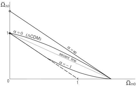
Figure 1: Schematic contour curves $\chi_{obs}=r_{inj}^{M}$ for $\alpha=-1,0$ and $\infty$, with $z_{obs}=\infty$ and $\Omega_{b0}=0$. The curves for intermediate values of $\alpha$ will interpolate monotonically between these extremes. Using $z_{obs}=1089$ instead does not change the curves significantly. The presence of baryonic matter prevents the $\alpha=-1$ curve from touching the flat line (dashed). The secant line (thin line) is a good approximation of the $\alpha=0$ curve.

For intermediate values of $\alpha$ we must turn to numerical integration to compute $\chi_{obs}$ and study quantitatively the effects of the GCG parameters on the detectability of the topology. We consider the set of topologies presented in Tables 1 and 2, and assess their (un)detectability based on current observational values of the cosmological density parameters and bounds on the parameter $\alpha$ of the GCG. We are particularly interested in the effect of the value of $\alpha$ on the potential detectability of the topology, as different values of $\alpha$ can be thought of as different models for the matter-energy content.

In the numerical computations we have set $\Omega_{b0}=0.04$ in equation (8). This value can be obtained from observations of light element abundances, combined with primordial Big-Bang nucleosynthesis analysis (Burles et al. BBN (2001), Kirkman et al. DH (2003)) and the value of the Hubble constant (Freedman freedman (2001)). For $\Omega_{0}$ we use the limits from a combination of CMBR and large-scale structure data obtained by Tegmark et al. (SDSSWMAP (2004)) for the $\Lambda$CDM case, $0.99<\Omega_{0}<1.03$. Finally we fix the total matter-like density parameter at $\bar{\Omega}_{m0}+\Omega_{b0}=0.3$. Our results however are not very sensitive to the precise value of $\bar{\Omega}_{m0}$. Indeed, for values of $\alpha$ not too negative ($\alpha>-0.5$), we have $\Delta\chi_{obs}/\chi_{obs}\simeq 0.15\,\Delta\bar{\Omega}_{m0}/\bar{\Omega}_{m0}$.

To quantify the dependency on $\alpha$ and $\Omega_{b0}$, we plot in figure (2) the depth $\chi_{obs}$ as a function of $\alpha$, for various values of $\Omega_{0}$. The plot with $\Omega_{b0}=0$ is shown in solid lines, and the plot with $\Omega_{b0}=0.04$ is given by the dashed lines.

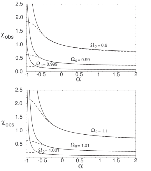
Figure 2: Survey depth $\chi_{obs}$, for several values of $\Omega_{0}=\Omega_{\mathrm{Ch}0}+\Omega_{b0}$, for hyperbolic (top) and spherical (bottom) universes, with $z_{obs}=1089$, and $\bar{\Omega}_{m0}+\Omega_{b0}=0.3$. The baryonic term is neglected in the solid lines and taken into account in the dashed lines.

The plots make clear a number of things. First, the value of $\chi_{obs}$ is not very sensitive to $\alpha$ for $\alpha>0$. Moreover, the change is very small for $\alpha>1$ ($\Delta\chi_{obs}/\chi_{obs}\simeq 0.3$ in the range $1\leq\alpha\leq\infty$). This implies that the undetectability conditions (3), which were derived for $\alpha\rightarrow\infty$, are not much more restrictive than the undetectabilty condition obtained in the case of the standard Chaplygin gas (i.e., $\alpha=1$). Note also that the presence of a small $\Omega_{b0}$ component does not change this picture in a significant way for positive values of $\alpha$. On the other hand, $\chi_{obs}$ changes substantially when $\alpha<0$. This was expected, since we have shown that if $\Omega_{b0}=0$ then $\chi_{obs}$ diverges in the limit $z\rightarrow\infty$ when $\alpha=-1$. The presence of a small amount of baryonic matter prevents this divergence, although $\chi_{obs}$ still changes appreciably for $\alpha<0$. It is clear then that for sufficiently negative values of $\alpha$, the precise value of $\Omega_{b0}$ plays an important role in the detection of cosmic topology in the GCG context.

In table 3 we display the manifolds from tables 1 and 2, along with their respective injectivity radii. The upper (for spherical manifolds) and lower (for hyperbolic ones) bounds on $\Omega_{0}$ so that the manifold’s topology is detectable in principle are shown in the table, for some noteworthy values of $\alpha$. We take the theoretical lower bound $\alpha=-1$; a numerical lower bound $\alpha=-1/2$ obtained from combining several observables and assuming a flat universe (see Makler et al. 2003b and Zhu Zhu (2004)); the $\Lambda$CDM case $\alpha=0$; and the standard Chaplygin Gas $\alpha=1$. The manifolds which are undetectable for $0.99\leq\Omega_{0}\leq 1.03$ are indicated with boldface.

Table 3: Minimum (maximum) values of $\Omega_{0}$ for each spherical (hyperbolic) topology to be potentially detectable (for $\bar{\Omega}_{M}=0.26,$ $\Omega_{b}=0.04$, and $z=1089$). Numbers in boldface indicate undetectabilty for the corresponding topologies.

Manifolds	$r_{inj}$	$\alpha=-1$	$\alpha=-0.5$	$\alpha=0$	$\alpha=1$
$D_{9}^{\ast},\ Z_{18}$	$\frac{\pi}{18}$	1.001	1.002	1.003	1.004
$D_{6}^{\ast},\ Z_{12}$	$\frac{\pi}{12}$	1.002	1.004	1.007	1.010
$I^{\ast},D_{5}^{\ast},\ Z_{10}$	$\frac{\pi}{10}$	1.003	1.005	1.010	1.015
$O^{\ast},D_{4}^{\ast},\ Z_{8}$	$\frac{\pi}{8}$	1.004	1.008	1.015	1.023
$T^{\ast},D_{3}^{\ast},\ Z_{6}$	$\frac{\pi}{6}$	1.007	1.014	1.026	1.042
$D_{2}^{\ast},\ Z_{4}$	$\frac{\pi}{4}$	1.016	1.031	1.059	1.094
m004(1,2)	0.183	0.999	0.998	0.997	0.995
m004(6,1)	0.240	0.998	0.997	0.994	0.991
m003(-4,3)	0.288	0.998	0.996	0.992	0.987
m003(-2,3)	0.289	0.998	0.996	0.992	0.987
m003(-3,1)	0.292	0.998	0.996	0.992	0.987
m009(4,1)	0.387	0.996	0.992	0.985	0.977
m007(3,1)	0.416	0.995	0.991	0.983	0.974

The table shows that the choice of $\alpha$ plays an important role in deciding on the detectability of these manifolds. In particular, negative values of $\alpha$ greatly favor detectability. All the manifolds above are potentially detectable for $\alpha=-1$, and all but $D_{2}^{\ast}$ and $Z_{4}$ are for $\alpha=-1/2$. In the case of $\alpha=1$, most of the selected hyperbolic and many of the singe action spherical manifolds are undetectable. It is clear that the detectability of individual topologies depends significantly on the value of $\alpha$, and in particular may greatly differ from the case of a $\Lambda$CDM model. This is an important point, inasmuch as it makes explicit the dependence of the detectability with respect to the model for the matter-energy content.

Of course one cannot list all the (infinite) manifolds in the dihedral and cyclic groups. These two classes are particularly important because as $\Omega_{0}\rightarrow 1$ from above, there is always an $n_{\ast}$ (or $m_{\ast}$) such that the topology corresponding to $Z_{n}$ (or $D_{m}^{\ast}$) is detectable in principle for $n>n_{\ast}$ (or $m>m_{\ast}$). We have seen that (3) provides a lower bound for $\chi_{obs}$ as a function of $\alpha$ and is also a fair approximation for the contour curves when $\alpha\geq 1$ for these manifolds. Solving (3) for $n_{\ast}$ and $m_{\ast}$ we can state that in a dihedral or lens space, for any value of $\alpha$ the topology is detectable (in principle) if

$$n_{\ast} \geq \mathrm{int}\left[\frac{\pi}{2}\frac{1}{\arctan(\sqrt{\Omega_{\mathrm{Ch}0}-1})}\right],$$

$$m_{\ast} \geq \mathrm{int}\left[\pi\frac{1}{\arctan(\sqrt{\Omega_{\mathrm{Ch}0}-1})}\right].$$ (16)

More specifically, for $\alpha\geq 1$ these are approximately equalities, since, as can be seen in Fig. 2, $\chi_{obs}$ is not very sensitive to the value of $\alpha$ for $\alpha\geq 1$. Recall that, although these expressions do not take baryons into account, their contribution is negligible for $\alpha\geq 1$. Thus, eqs. (3) provide an absolute lower bound for the detectability of cyclic and dihedral topologies. Any values of $n$ and $m$ greater than $n_{\ast}$ and $m_{\ast}$, respectively, will render the topology potentially detectable for any value of $\alpha$.

Given the increasing amount of high quality cosmological data, in particular the availability of high resolution full sky CMBR maps (see Spergel et al. WMAP-Spergel-et-al (2003)), we can expect to detect a non-trivial topology if it is present and if $r_{inj}<\chi_{obs}$. This can be done, for example, by observing matching circles in the CMBR maps. Indeed some topological signatures have recently been proposed and tested (see Luminet et al. Poincare (2003), Cornish et al. Cornishetal03 (2004), Roukema et al. Roukema (2004), and Aurich et al Aurich (2005)). One can then ask whether the hypothetical detection of a nontrivial topology may lead to a better knowledge of the cosmological model. In the case of the GCG, does the determination of a given topology impose any constraint on $\alpha$?

The answer is positive, as can be seen from figure (3). There we plot the contour curves $\chi_{obs}(\Omega_{0},\alpha)=r_{inj}^{\;M}$, in the $\Omega_{0}-\alpha$ parametric plane for the same topologies discussed in the previous section, where we fix $z_{obs}=1089$, $\Omega_{b0}=0.04$ and $\bar{\Omega}_{m0}=0.26$. Recall from section (3) that each such contour curve separates the parametric plane in two regions where the manifold in question is respectively potentially detectable and undetectable. It is clear, for example, that the detection of a binary tetrahedral topology ($T^{\ast}$) would place the constraint $\alpha<-0.2$ for current bounds on $\Omega_{0}$. If future observations tighten the range of $\Omega_{0}$ even closer to $1$, let’s say $\Omega_{0}=1.000\pm 0.003$, the detection of either $D_{9}^{\ast},\ Z_{18}$, m$004(1,2)$, or m$004(6,1)$ would imply $\alpha\lesssim-0.5$.

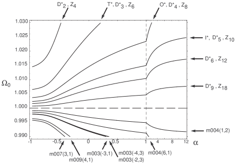
Figure 3: Curves of constant $\chi_{obs}=r_{inj}^{\;M}$, in the ($\Omega_{0}$, $\alpha$) plane for the same topologies discussed in the previous section. The $\alpha$ axis is compressed for $1\leq\alpha\leq 12$. Again we fix $z=1089$, and $\bar{\Omega}_{m0}+\Omega_{b0}=0.3$, with $\Omega_{b0}=0.04$.

Figure (3) shows that a topology that would be detectable in a $\Lambda$CDM universe is not necessarily ruled out if no observational topological signature is found. For example, if no sign is detected of the binary octahedral ($O^{\ast}$) topology in CMBR maps, it could simply be that $\alpha\gtrsim 2.5,$ so that this topology is in fact unobservable in the $\Lambda$CDM context.

4 Discussion and concluding remarks

We have considered the detectability of a non-trivial cosmic topology in a universe dominated by the GCG. This component offers the possibility of dark-matter/energy unification and is consistent with a number of cosmological observations. We have investigated how the detectability is altered with respect to changes in the model parameters, as well as to the choice of the model itself, using the GCG family as a concrete example.

In the case of the $\Lambda$CDM model, the detectablity of a manifold’s topology is a function of the component densities, $\Omega_{m0}$ and $\Omega_{\Lambda 0}$. The consideration of the GCG brings in a new parameter into the analysis, the steepness of the equation of state $\alpha$. We have shown that, for fixed $\Omega_{0}$ and $\bar{\Omega}_{m0}$, more topologies become potentially detectable as $\alpha$ decreases. We have obtained analytical results for $\alpha\rightarrow\infty$, establishing a lower bound for the detectability in the GCG case. In general, the detectability is not very sensitive to $\alpha$, for $\alpha>0$, but varies greatly for negative values of $\alpha$. In this latter case, the contribution of baryons is important and must be taken into account. For example, we have shown that for $\alpha=-1$ any topology would be potentially detectable if we neglect $\Omega_{b0}$. However, considering the baryonic contribution, many manifolds would still be unobservable.

It is now possible to expect detectable non-trivial topologies to leave a measurable imprint on CMBR maps. The detection of a cosmic topology is therefore a realistic possibility in the near future, and we have investigated what constraints would be imposed on the parameters of the model, by such a detection. For example, the hypothetical detection of a binary tetrahedral topology would place the constraint $\alpha<-0.2$ for $\Omega_{0}<1.02$, $\bar{\Omega}_{m0}=0.26$, and $\Omega_{b}=0.04$. A more thorough study of the inverse problem is developed in Makler et al. (paperGCGtopology (2005)).

In the present work we outline a method for studying the detectability of cosmic topology systematically for a family of cosmological models. Although this method was applied to the GCG model for DM and DE unification, it can be used to study other models or choices of variables. For instance, a more physically motivated parametrization might be to use $\Omega_{m0}^{eff}=\Omega_{\mathrm{Ch}0}\left(1-A\right)^{1/\left(1+\alpha\right)}+\Omega_{b}$, which is the fraction that behaves as CDM for early times and is measured from the matter clustering. This variable is more directly constrained by some observational data (see Makler et al. 2003b and Reis et al. entropy (2003)), and may be better suited for studies involving comparisons with observational constraints. This choice of variables is adopted in Makler et al. (paperGCGtopology (2005)).

An important point that emerges from these results is that given a set of observational constraints, the detectability of cosmic topology depends on the choice of the cosmological model. Thus, any attempt to rule out a given topology must take this into account.

- (1) Aurich, R., Lustig, S. & Steiner, F. 2005, astro-ph/0412569
- (2) Bento, M.C., Bertolami, O. & Sen, A.A. 2002, Phys. Rev. D 66, 043507
- (3) Bertone, G., Hooper, D. & Silk, J. 2005, Phys. Rept. 405, 279
- (4) Bilić, N., Tupper, G.B. & Viollier, R.D. 2002, Phys. Lett. B 535, 17
- (5) Burles, S., Nollett, K.M. & Turner, M.S. 2001, ApJ 552, L1
- (6) Cornish, N.J., Spergel, D.N. & Starkman, G.D. 1998, Class. Quant. Grav. 15, 2657
- (7) Cornish, N.J., Spergel, D.N. & Starkman, G.D. 2004, Phys. Rev. Lett. 92, 201302
- (8) Dev, A., Jain, D. & Alcaniz, J. S. 2004, AA 417, 847
- (9) Ellis, G.F.R. 1971, Gen. Rel. Grav. 2, 7
- (10) Freedman, W. 2001, AJ 553, 47
- (11) Gausmann, E., Lehoucq, R., Luminet, J.-P., Uzan, J.-P. & Weeks, J. 2001, Class. Quant. Grav. 18, 5155
- (12) Gomero, G.I., , Rebouças, M.J. & Tavakol, R. 2001, Class. Quantum Grav. 18, 4461
- (13) Gomero, G.I., , Rebouças, M.J. & Teixeira, A.F.F. 2001, Class. Quantum Grav. 18, 1885
- (14) Hodgson, C.D. & Weeks, J.R. 1994, Experimental Mathematics 3, 261
- (15) Kamenshchik, A., Moschella, U. & Pasquier, V. 2001, Phys. Lett. B 511, 265
- (16) Kirkman, D., Tytler, D., Suzuki, N.J., O’Meara, M. & Lubin, D. 2003, ApJ Suppl. 149, 1
- (17) Lachièze-Rey, M. & Luminet, J.-P. 1995, Phys. Rep. 254, 135
- (18) Lehoucq, R., Lachièze-Rey, M. & Luminet, J.-P. 1996, AA 313, 339
- (19) Levin, J. 2002, Phys. Rep. 365, 251
- (20) Luminet, J.-P., Weeks, J., Riazuelo, A., Lehoucq, R. & Uzan, J.-P. 2003, Nature 425, 593
- (21) Makler, M. 2001 Gravitational Dynamics of Structure Formation in the Universe, PhD Thesis, Brazilian Center for Research in Physics
- (22) Makler, M., Oliveira, S.Q. & Waga, I. 2003, Phys. Lett. B 555, 1
- (23) Makler, M., Oliveira, S.Q. & Waga, I. 2003, Phys. Rev. D 64, 123521
- (24) Makler, M., Mota, B. & Rebouças, M.J., to appear in Proceedings of the Xth Marcel Grossman Meeting
- (25) Makler, M., Mota, B. & Rebouças, M.J. 2005, submitted for publication
- (26) Mota, B., Rebouças, M.J. & Tavakol, R. 2003, Class. Quantum Grav. 20, 4837
- (27) Mota, B., Gomero, G.I., Rebouças, M.J. & Tavakol, R. 2004, Class. Quantum Grav. 21, 3361
- (28) de Oliveira-Costa, A., Tegmark, M., Zaldarriaga, M. & Hamilton, A. 2004, Phys. Rev. D 69, 063516
- (29) Perlmutter, S., et al. 1998, Nature 391, 51
- (30) Rebouças, M.J. & Gomero, G.I. 2004, Braz. J. Phys. 34, 1358; astro-ph/0402324
- (31) Reis, R.R.R., Waga, I., Calvão, M.O. & Jorás, S. E. 2003, Phys. Rev. D 68, 061302
- (32) Riess, A.G., et al. 1998, AJ, 116, 1009
- (33) Roukema, B.F., Bartosz, L., Cechowska, M., Marecki, A. & Bajtlik, S. 2004, AA 423, 821
- (34) Spergel, D.N. et al. 2003, ApJ Suppl. 148, 175
- (35) Starkman, G.D. 1998, Class. Quantum Grav. 15, 2529
- (36) Tegmark, M., et al. 2004, Phys. Rev. D 69, 103501
- (37) Tonry, J.L., et al. 2003, AJ 594, 1
- (38) Threlfall, W. & Seifert, H. 1932, Math. Annalen 104, 543
- (39) Uzan, J.-P. , Lehoucq, R. & Luminet, J.-P. 1999, AA 351, 766
- (40) Weeks, J.R. 1999, SnapPea: A computer program for creating and studying hyperbolic 3-manifolds, available at http://geometrygames.org/SnapPea/
- (41) Weeks, J.R. 2003, Mod. Phys. Lett. A 18, 2099
- (42) Weeks, J.R., Lehoucq, R. & Uzan, J-P. 2003, Class. Quant. Grav. 20, 1529
- (43) Wolf, J.A. 1984, Spaces of Constant Curvature, fifth ed., Publish or Perish Inc., Delaware
- (44) Zhu, Z.-H. 2004, AA 423, 421