Soft coincidence in late acceleration

Abstract

We study the coincidence problem of late cosmic acceleration by assuming that the present ratio between dark matter and dark energy is a slowly varying function of the scale factor. As dark energy component we consider two different candidates, first a quintessence scalar field, and then a tachyon field. In either cases analytical solutions for the scale factor, the field and the potential are derived. Both models show a good fit to the recent magnitude-redshift supernovae data. However, the likelihood contours disfavor the tachyon field model as it seems to prefer a excessively high value for the matter component.

I Introduction

Nowadays it is widely accepted that the present stage of cosmic expansion is accelerated reviews ; adam albeit there are rather divergent proposals about the mechanism behind this acceleration. A cosmological model of present acceleration should not only fit the high redshift supernovae data, the cosmic microwave background anisotropy spectrum and safely pass other tests, it must solve the coincidence problem as well, namely “why the Universe is accelerating just now?”, or in the realm of Einstein gravity “why are the densities of matter and dark energy of precisely the same order today?” coincidence -note that these two energies scale differently with redshift. While it might happen that this coincidence is just a “coincidence” -and as such no explanation is to be found- we believe models that fail to account for this cannot be regarded as satisfactory.

In a class of models designed to solve this problem the dark energy density “tracks” the matter energy density for most of the history of the Universe, and overcomes it only recently (see, e.g., Ref. trackers ). However, these models suffer the drawback of fine-tuning the initial conditions whereupon they are not, after all, much better than the conventional “concordance” model which rests on a mixture of matter and a fine-tuned cosmological constant sabino .

There is an especially successful subset of models based on an interaction between dark energy and cold matter (i.e., dust) such that the ratio $r$ of the corresponding energy densities tends to a constant of order unity at late times plb ; luca ; scale ; interacting ; dw ; somasri ; olivares thus solving the problem. However, the current observational information does not necessarily imply that $r$ ought to be strictly constant today. For the coincidence problem to be addressed a softer condition may suffice, namely that at present $r$ should be a slowly varying function of the scale factor with $r(a=a_{0})\simeq 3/7$, the currently observed ratio. By slowly varying we mean that the current rate of variation of $r(a)$ should be no much larger than $H_{0}$, where $H\equiv\dot{a}/a$ denotes the Hubble factor of the Friedamnn-Lemaitre-Robertson-Walker (FLRW) metric, and a zero subscript means present time. It should be noted that because the nature of dark matter and dark energy is largely unknown an interaction between both cannot be excluded a priori. In fact, the possibility has been suggested from a variety of angles angles .

To avoid a possible conflict with observational constraints on long-range forces only we consider that the baryon component of the matter does not participate in the the interaction and, further, to simplify the analysis -i.e., in order not to have an uncoupled component- we exclude the baryons altogether. While this might be seen as a radical step it should be taken into account that our study restricts itself to times near the present time and these are characterized, among other things, by a low value of the baryon energy density ($5$% or less of the total energy budget, approximately six times lower than the dark matter contribution and fourteen below the dark energy component spergel ) whereby it should not significantly affect our results. This is in keeping with the findings of Majerotto et al. majerotto . For interacting models encompassing most the Universe history in which the baryons enter the dynamical equations as a non-interacting component, see Refs. majerotto and luca .

The target of this paper is to present two models of late acceleration that fulfill “soft coincidence”, namely: $(i)$ when the dark energy is a quintessence scalar field, and $(ii)$ when the dark energy is a tachyon field. The latter was introduced by Sen sen and soon afterwards it became a candidate for driving inflation as well as late acceleration -see e.g., Ref. gary . The outline of this paper is as follows: Section II considers the quintessence model with a constant equation of state parameter. There it is assumed that the quintessence field slowly decays into dark matter with the equation of state of dust. Section III considers the tachyon field and again assumes a slowly decay into dust. This time, however, the equation of state parameter is allowed to vary. Finally, section IV summarizes our findings.

II The quintessence interacting model

We consider a two-component system, namely, cold dark matter, described by an energy density $\rho_{m}$, and a quintessence scalar field $\phi$ with energy density and pressure defined by

$$\rho_{\phi}=\textstyle{1\over{2}}\dot{\phi}^{2}+V(\phi)\,,\qquad\mbox{and}\qquad p_{\phi}=\textstyle{1\over{2}}\ \dot{\phi}^{2}-V(\phi),$$ (1)

respectively, in a spatially flat FLRW universe. The over dot indicates derivative with respect to the cosmic time and $V(\phi)$ is the quintessence scalar potential. We assume that these two components do not evolve separately but interact through a source (loss) term (say, $Q$) that enters the energy balances

$$\dot{\rho}_{m}+3H\rho_{m}=Q$$ (2)

and

$$\dot{\rho}_{\phi}+3H(\rho_{\phi}+p_{\phi})=-Q,$$ (3)

where in view of (1) last equation is equivalent to

$$\dot{\phi}\left[\ddot{\phi}+3H\dot{\phi}+V^{\prime}\right]=-Q.$$ (4)

In the following we constrain the interaction $Q$ by demanding that the solution to Eqs. (2) and (3) be compatible with a variable ratio between the energy densities $r(x)\equiv\rho_{m}/\rho_{\phi}$, where $x=a/a_{0}$ is the normalized scale factor, and that around the present time $r(x)$ is a smooth, nearly constant function with $r(x=1)=r_{0}$ being of order one. We also assume that the quintessence component obeys a barotropic equation of state, it is to say $p_{\phi}=w_{\phi}\rho_{\phi}$ with $w_{\phi}$ a negative constant (a distinguishing feature of dark energy fields -quintessence fields or whatever- is a high negative pressure). In virtue of these relations the set of dynamical equations reduces to a single equation

$$\dot{\rho}_{\phi}+3H\left(1+\frac{w_{\phi}+\frac{\dot{r}}{3H}}{1+r}\right)\rho_{\phi}=0\,,$$ (5)

whose solution is

$$\rho_{\phi}(x)=\rho_{\phi}^{(0)}\,e^{-3I(x)},$$ (6)

with

$$I(x)=\int_{1}^{x}{F(x^{\prime})\frac{dx^{\prime}}{x^{\prime}}}\,,\quad\mbox{where}\,\quad F(x)=1+\frac{w_{\phi}+{\textstyle{1\over 3}}xr^{\prime}(x)}{1+r(x)}\,,$$ (7)

and the prime means derivation with respect to $x$. On the other hand, by combining Friedmann’s equation

$$3H^{2}=\kappa(\rho_{m}+\rho_{\phi})\qquad(\kappa\equiv 8\pi G)$$ (8)

with Eq. (6) we get

$$H(x)=H_{0}\,\sqrt{\frac{1+r(x)}{1+r_{0}}}\,e^{-\frac{3}{2}I(x)},$$ (9)

where $H_{0}=\sqrt{\rho_{\phi}^{(0)}\kappa/3}$ denotes the current value of the Hubble factor. From this, it follows that

$$\frac{H_{0}}{\sqrt{1+r_{0}}}\left[t(x)-t_{0}\right]=\int_{1}^{x}{\frac{e^{\frac{3}{2}I(x^{\prime})}}{\sqrt{1+r(x^{\prime})}}\frac{dx^{\prime}}{x^{\prime}}}.$$ (10)

If this integral could be solved analytically, we would obtain the scale factor in terms of the cosmological time.

Equations (3) and (5) alongside  (6),  (7), and  (9) imply

$$Q(x)=\frac{3H_{0}\rho_{\phi}^{(0)}}{\sqrt{1+r_{0}}}\,\frac{1}{\sqrt{1+r(x)}}\,\left[\frac{x\,r^{\prime}(x)}{3}-w_{\phi}\,r(x)\right]\,e^{-\textstyle{9\over{2}}I(x)}.$$ (11)

Note that $Q(x)$ is a positive-semidefinite function, as it should. A negative $Q(x)$ would imply a transfer of energy from the matter to the scalar field which migth violate the second law of thermodynamics. While in view of the unknown nature of dark matter and dark energy we cannot say for certain that these components fulfill the aforesaid law, in the absence of any evidence against it, the most natural thing is to assume that they obey it.

From the definitions (1) and the equation of state $p_{\phi}=w_{\phi}\rho_{\phi}$ the quintessence field and its potential are given by

$$\phi(x)=\phi_{0}+\sqrt{\frac{3(1+w_{\phi})}{\kappa}}\int_{1}^{x}{\sqrt{\frac{1}{1+r(x^{\prime})}}\,\frac{dx^{\prime}}{x^{\prime}}},$$ (12)

and

$$V(x)=V_{0}\,e^{-3I(x)},$$ (13)

respectively. Here $\phi_{0}$ is an integration constant, and $V_{0}=\textstyle{1\over{2}}\left(1-w_{\phi}\right)\rho_{\phi}^{(0)}$.

As said before, we apply the above formalism to the case in which the variable $x$ is not far from unity whence the ratio $r(x)$ can be approximated by

$$r(x)\simeq r_{0}+\varepsilon_{0}(1-x),$$ (14)

where $r_{0}$ is the present value of the ratio between the energy densities $\rho_{m}$ and $\rho_{\phi}$, and $\varepsilon_{0}$ is a small positive-definite constant. We do not consider negative values for $\varepsilon_{0}$ since it would imply that $r(x)$ was increasing in the recent past and therefore that it oscillates. While we are unaware of any definitive argument against this possibility it looks certain that only contrived models may lead to this behavior. Further, oscillations in $r(x)$ may seriously jeopardize the well tested picture of structure formation springel . (Note in passing that the choice (14) implies that $\mid\dot{r}(x)\mid\lesssim H_{0}$ for $x\sim{\cal O}(1)$).

It follows that

$$F(x)=1+\frac{\alpha_{1}-\alpha_{2}x}{\alpha_{3}-\alpha_{4}x}\,,$$ (15)

where the $\alpha_{i}$ are constants given by

$$\alpha_{1}=w_{\phi},\quad\alpha_{2}=\textstyle{1\over{3}}\varepsilon_{0},\quad\alpha_{3}=1+r_{0}+\varepsilon_{0},\quad\alpha_{4}=\varepsilon_{0},$$ (16)

respectively. With this, we obtain

$$\rho_{m}(x)=\rho_{\phi}^{(0)}\left(\frac{\alpha_{3}-\alpha_{4}}{\alpha_{3}-\alpha_{4}x}\right)(\alpha_{3}-1-\alpha_{4}\,x)\,x^{-3\left(\frac{\alpha_{1}+\alpha_{3}}{\alpha_{3}}\right)}.$$ (17)

and

$$\rho_{\phi}(x)=\rho_{\phi}^{(0)}\left(\frac{\alpha_{3}-\alpha_{4}}{\alpha_{3}-\alpha_{4}x}\right)\,x^{-3\left(\frac{\alpha_{1}+\alpha_{3}}{\alpha_{3}}\right)},$$ (18)

The Hubble parameter can be written as

$$H(x)=H_{0}\,x^{-\frac{3}{2}\left(\frac{\alpha_{1}+\alpha_{3}}{\alpha_{3}}\right)},$$ (19)

where $H_{0}$ was given above. From this expression the scale factor is shown to follow a power-law dependence on time

$$a(t)=a_{0}\left(\frac{t}{t_{0}}\right)^{\frac{2\,\alpha_{3}}{3(\alpha_{1}+\alpha_{3})}}.$$ (20)

For the Universe to accelerate, the constraint $\frac{2\,\alpha_{3}}{3\left(\alpha_{1}+\alpha_{3}\right)}>1$ must be fulfilled, i.e.,

$$1+r_{0}+\varepsilon_{0}<-3w_{\phi}.$$ (21)

This, alongside the condition that the energy densities decrease with expansion implies

$$-w_{\phi}<1+r_{0}+\varepsilon_{0}<-3w_{\phi}.$$ (22)

Fig. 1 shows a good fit to the “gold” set of supernovae data points of Riess et al. adam .

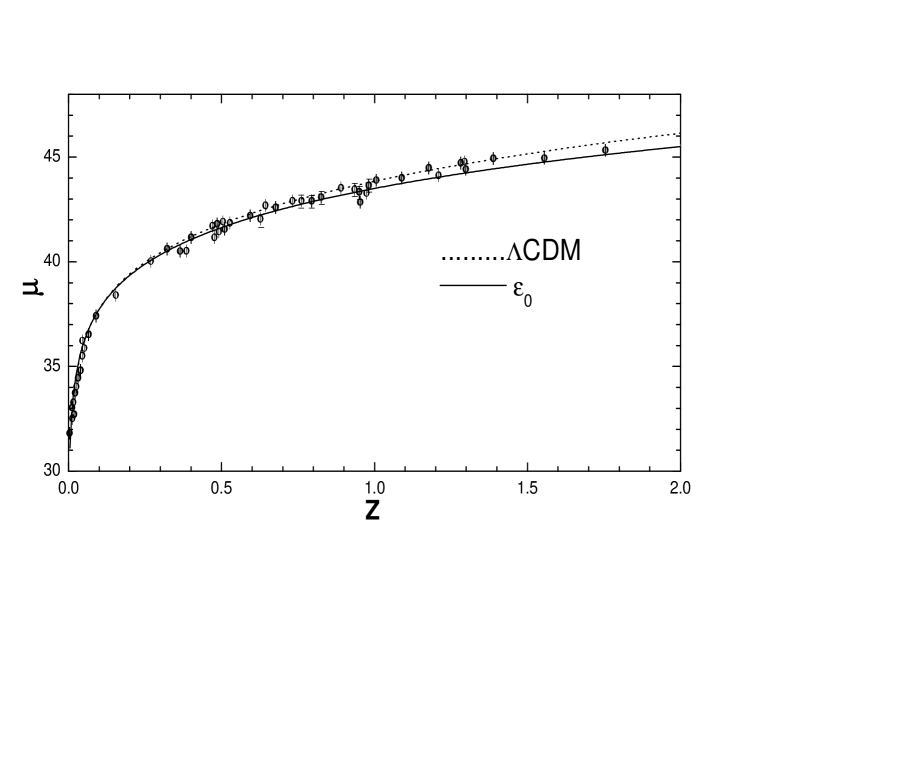
Figure 1: Distance moduli vs redshift for the quintessence–dark matter interacting model. In plotting the graphs the expression $\mu=5\log d_{L}+25$, with $d_{L}=(1+z)\int^{z}_{0}H^{-1}(z^{\prime})dz^{\prime}$ in units of megaparsecs was assumed. Here $w_{\phi}=-0.75$, $\varepsilon_{0}=0.077$ and $r_{0}=0.27$. For comparison we have also plotted the prediction of the concordance $\Lambda$CDM model with $\Omega_{m0}=0.3$. The data points correspond to the “gold” sample of type Ia supernovae of Ref. adam .

The likelihood contours are depicted in Fig. 2. The mean values of the free parameters are: $\Omega_{\phi}=0.78538$, $w_{\phi}=-0.757284$, $\varepsilon_{0}=0.0777764$. Notice that $\Omega_{\phi}$ is above the concordance $\Lambda$CDM value of $0.73$ and that $w_{\phi}$ is significantly larger than the value found in non-interacting models. However, we have not considered phantom fields (scalar fields as given by Eq. (1) do not encompass phantom behavior), otherwise a shift of $w_{\phi}$ toward more negative values should be expected. Notice (top panels) that the parameter $\varepsilon_{0}$ is rather degenerate.

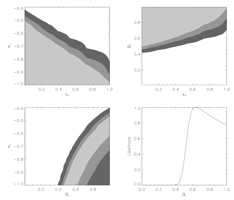
Figure 2: Likelihood contours for the quintessence–matter interacting model showing the 68%, 90% and 99% confidence intervals. The likelihoods are marginalized over the rest of parameters. The prior $\Omega_{m}+\Omega_{\phi}=1$ was used. The right bottom panel shows the probability function of the quintessence parameter density.

Under restriction  (21) the interaction term reads

$$Q(x)=-3H_{0}\rho_{\phi}^{(0)}\left[w_{\phi}+\frac{\alpha_{4}x}{3[(\alpha_{3}-1-\alpha_{4}x)]}\right](\alpha_{3}-\alpha_{4})\frac{\left(\alpha_{3}-1-\alpha_{4}x\right)}{\left(\alpha_{3}-\alpha_{4}x\right)^{2}}\,x^{-\textstyle{9\over{2}}\left(\frac{\alpha_{1}+\alpha_{3}}{\alpha_{3}}\right)},$$ (23)

see Fig. 3.

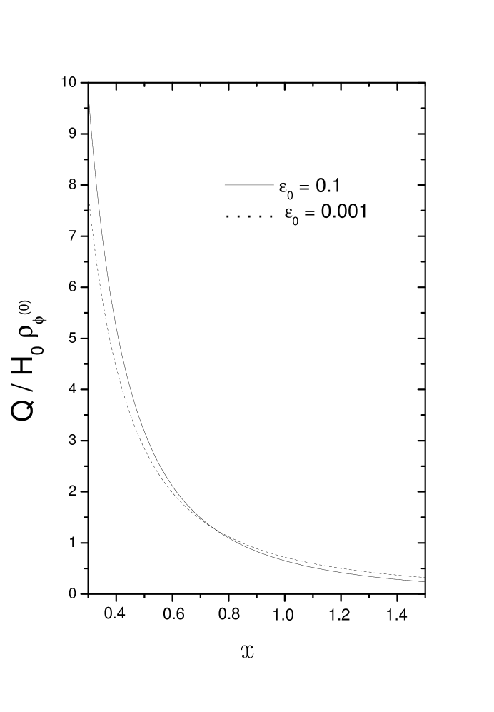
Figure 3: Evolution of the interaction term with expansion. The lower $\varepsilon_{0}$, the slower the decrease of the quintessence field. Here $w_{\phi}=-0.8$ and $r_{0}=3/7$

.

In its turn, the scalar field $\phi$ and the scalar potential $V(x)$ are given by

$$\phi(x)=\phi_{0}\left[\frac{\tanh^{-1}\left(\sqrt{1-\frac{\alpha_{4}}{\alpha_{3}}x}\right)}{\tanh^{-1}\left(\sqrt{1-\frac{\alpha_{4}}{\alpha_{3}}}\right)}\right]\,,$$ (24)

and

$$V(x)=V_{0}\left(\frac{\alpha_{3}-\alpha_{4}}{\alpha_{3}-\alpha_{4}x}\right)\,x^{-3\left(\frac{\alpha_{1}+\alpha_{3}}{\alpha_{3}}\right)},$$ (25)

respectively. Here $\phi_{0}=\sqrt{\frac{12}{\kappa}\left(\frac{1+w_{\phi}}{\alpha_{3}}\right)}\tanh^{-1}\left[\sqrt{1-\frac{\alpha_{4}}{\alpha_{3}}}\right]$, and $V_{0}=\textstyle{1\over{2}}(1-w_{\phi})\rho_{\phi}^{(0)}$, see Fig. 4.

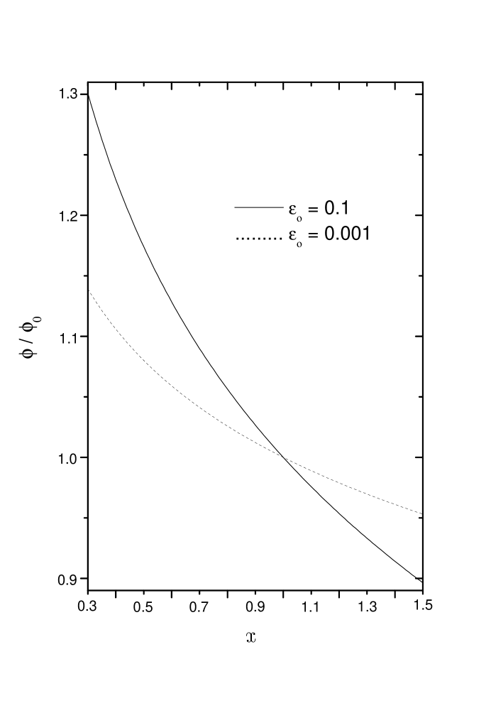
Figure 4: Evolution of the scalar field with expansion. Again, $w_{\phi}=-0.8$ and $r_{0}=3/7$.

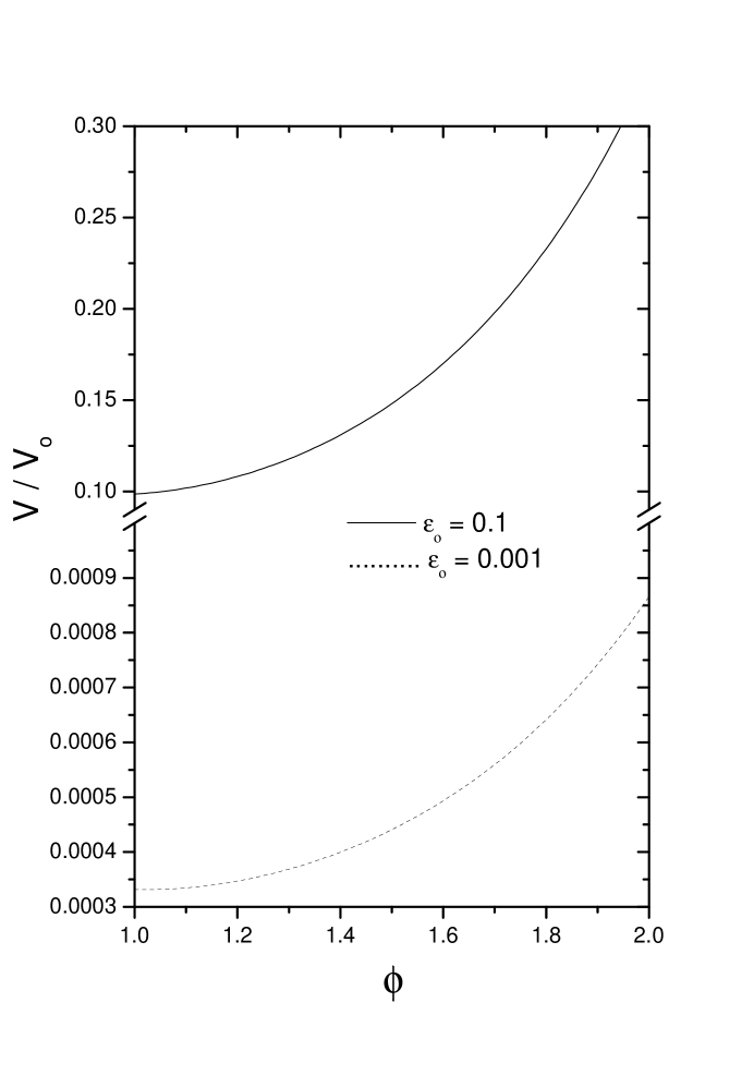
Figure 5: The effective potential versus the scalar field. Here $w_{\phi}=-0.8$ and $r_{0}=3/7$.

Equations  (24) and (25) lead to

$$V(\phi)=\frac{V_{0}\left(1-\frac{\alpha_{4}}{\alpha_{3}}\right)}{\tanh^{2}\left(\sqrt{\frac{\kappa\alpha_{3}}{12\left(1+w_{\phi}\right)}}\,\phi\right)}\,\left[\sqrt{\frac{\alpha_{3}}{\alpha_{4}}}\,\,\mbox{sech}\left(\sqrt{\frac{\kappa\alpha_{3}}{12\left(1+w_{\phi}\right)}}\,\phi\right)\right]^{-6\left(\frac{\alpha_{1}+\alpha_{3}}{\alpha_{3}}\right)}\,.$$ (26)

Figures 4 and 5 taken together show that the potential decreases with the Universe expansion. While we do not know whether there is any field theory backing this potential it is intriguing to see that around $\phi=0$ it behaves as

$$V(\phi)\sim C_{1}\phi^{-2}+C_{2}+C_{3}\phi^{2}+C_{4}\phi^{4}+...\,$$ (27)

where the $C_{i}$’s are constants. The first term is used in quitessence models -see e.g., Ref. potentials , whereas the third and fourth terms of the expansion are well–known potentials in inflation theory (chaotic potentials) Linde ; the second term plays the role of a cosmological constant. This leads us to surmise that, in reality, $V(\phi)$ might be considered an effective potential resulting from the combination of a number of fields.

III The tachyon interacting model

The tachyon field naturally emerges as a straightforward generalization of the Lagrangian of the relativistic particle much in the same way as the scalar field $\phi$ arises from generalizing the Lagrangian of the non–relativistic particle bagla . Recently, the realization of its potentiality as dark matter shiu and dark energy awakened has awakened the interest in it. We begin by succinctly recalling the basic equations of the tachyon field to be used below where its interaction with cold dark matter (dust) will be considered.

The stress–energy tensor of the tachyon field

$$T^{(\varphi)}_{ab}=\frac{V(\varphi)}{\sqrt{1+{\varphi}^{,c}{\varphi}_{,c}}}\left[-g_{ab}\left(1+{\varphi}^{,c}{\varphi}_{,c}\right)+\varphi_{,a}\varphi_{,b}\right]\ ,$$ (28)

admits to be written in the perfect fluid form

$$T^{(\varphi)}_{ab}=\rho_{\varphi}u_{a}u_{b}+p_{\varphi}\left(g_{ab}+u_{a}u_{b}\right),$$ (29)

where the energy density and pressure are given by

$$\rho_{\varphi}=\frac{V(\varphi)}{\sqrt{1-\dot{\varphi}^{2}}}\,,\qquad\mbox{and}\qquad p_{\varphi}=-V(\phi){\sqrt{1-\dot{\varphi}^{2}}},\$$ (30)

respectively, with

$$\dot{\varphi}\equiv\varphi_{,a}u^{a}=\sqrt{-g^{ab}\varphi_{,a}\varphi_{,b}}\,,\quad\mbox{and}\quad u_{a}=-\frac{\varphi_{,a}}{\dot{\varphi}}\ ,\quad\mbox{where}\quad u^{a}u_{a}=-1.$$ (31)

In the absence of interactions other than gravity the evolution of the energy density is governed by $\dot{\rho}_{\varphi}=-3H\dot{\varphi}^{2}\rho_{\varphi}$, therefore when $\dot{\varphi}^{2}<1$ it decays at a lower rate than that for dust. It approaches the behavior of dust for $\dot{\varphi}^{2}\rightarrow 1$, thereby in this limit the tachyon field behaves dynamically as pressureless matter does. Consequently, we shall assume $\dot{\varphi}^{2}<1$ since for $\dot{\varphi}^{2}=1$ both components obey the same equation of state for dust.

For an interacting mixture of a tachyon field and cold dark matter, with energy density $\rho_{m}$ and negligible pressure, the interaction term, $Q$, between these two components is described by the following balance equations

$$\dot{\rho}_{m}+3H(\rho_{m}+\Pi_{m})=Q\ ,$$ (32)

$$\dot{\rho}_{\varphi}+3H\dot{\varphi}^{2}\rho_{\varphi}=-Q\,.$$ (33)

The $\Pi_{m}$ term, on the left hand side of Eq. (32), accounts for the fact that the matter component may be endowed with a viscous pressure or perhaps it is slowly decaying into dark matter and/or radiation decay . In either case one can model this term as $\Pi_{m}=\alpha\rho_{m}H$ with $\alpha$ a small negative constant since $\Pi_{m}$ is a small correction to the matter pressure -see winfried and references therein.

As before, we consider the ratio between the densities of matter and tachyonic energy a function $r(x)$ of the normalized scale factor (to be specified later), and again, we must have $Q(x)>0$ -its expression is to be found below. Then, equations  (32) and (33) combine to

$$\dot{\rho}_{\varphi}+3H\left[1+\frac{w_{\varphi}+\alpha r(x)+\frac{r^{\prime}(x)\,x}{3}}{1+r(x)}\right]\rho_{\varphi}=0\qquad(x\equiv a/a_{0})\,.$$ (34)

The latter can be solved to

$$\rho_{\varphi}(x)=\rho_{\varphi}^{(0)}e^{-3\tilde{I}(x)}\,,\qquad\mbox{where}\qquad\tilde{I}(x)=\int_{1}^{x}{\tilde{F}(x^{\prime})\,\frac{dx^{\prime}}{x^{\prime}}},$$ (35)

with

$$\tilde{F}(x)=1+\frac{w_{\varphi}(x)+\alpha r(x)+\textstyle{1\over{3}}r^{\prime}(x)x}{1+r(x)}.$$ (36)

The interaction term takes the form

$$Q(x)=3\rho_{\varphi}^{(0)}H(x)\left(\frac{r(x)}{1+r(x)}\right)\left[\alpha-w_{\varphi}(x)+\frac{xr^{\prime}(x)}{3r(x)}\right]e^{-3\tilde{I}(x)}.$$ (37)

and the tachyonic scalar field and its potential obey

$$\varphi(x)=\varphi_{0}+\frac{\sqrt{1+r_{0}}}{H_{0}}\int_{1}^{x}{\sqrt{\frac{1+w_{\varphi}(x^{\prime})}{1+r(x^{\prime})}}\,e^{\frac{3}{2}\tilde{I}(x^{\prime})}}\,\frac{dx^{\prime}}{x^{\prime}},$$ (38)

and

$$V(x)=V_{0}\sqrt{-w_{\varphi}(x)}\,\,e^{-3\tilde{I}(x)},$$ (39)

respectively.

Up to now we have left the ratio function $r(x)$ free. As before, we specify it for $x$ values around unity as

$$r(x)\simeq r_{0}+\varepsilon_{0}(1-x),$$ (40)

where $r_{0}=(\rho_{m}/\rho_{\varphi})_{0}$, and $\varepsilon_{0}$ is once again a small positive-definite constant. Likewise, we assume that the equation of state parameter $w_{\varphi}$ is given by

$$w_{\varphi}(x)=w_{0}+w_{1}(1-x),$$ (41)

where $w_{0}$ and $w_{1}$ are constants, the first one denotes the current value of the $w_{\varphi}(x)$ function, and the second one is minus its first derivative, which is expected to be small. Thus,

$$\tilde{F}(x)=1+\frac{a_{1}-b_{1}x}{a_{2}-b_{2}x},$$ (42)

where the constants $a_{i}$ and $b_{i}$ stand for

$$a_{1}=\alpha r_{0}+w_{0}+w_{1}+\varepsilon_{0},\qquad a_{2}=1+r_{0}+\varepsilon_{0}$$ (43)

and

$$b_{1}=w_{1}+(\alpha+\textstyle{1\over{3}})\varepsilon_{0},\qquad b_{2}=\varepsilon_{0},$$ (44)

respectively. It follows that

$$\rho_{m}(x)=\rho_{\varphi}^{(0)}\,(1+r_{0})^{3\beta_{1}}\,x^{-3\beta_{2}}\,[r_{0}+\varepsilon_{0}(1-x)]\,[1+r_{0}+\varepsilon_{0}(1-x)]^{-3\beta_{1}}\,,$$ (45)

as well as

$$\rho_{\varphi}(x)=\rho_{\varphi}^{(0)}\,(1+r_{0})^{3\beta_{1}}\,x^{-3\beta_{2}}\,[1+r_{0}+\varepsilon_{0}(1-x)]^{-3\beta_{1}},$$ (46)

with

$$\beta_{1}=\frac{b_{1}}{b_{2}}-\frac{a_{1}}{a_{2}}=\frac{w_{1}}{\varepsilon_{0}}+\left(\alpha+\textstyle{1\over{3}}\right)-\left[\frac{\alpha r_{0}+w_{1}+w_{0}+\varepsilon_{0}}{1+r_{0}+\varepsilon_{0}}\right],$$

and

$$\beta_{2}=1+\frac{a_{1}}{a_{2}}=\frac{1+w_{1}+2\varepsilon_{0}+r_{0}(1+\alpha)}{1+r_{0}+\varepsilon_{0}}\,.$$

The Hubble function

$$H(x)=H_{0}\,(1+r_{0})^{\frac{3\beta_{1}-1}{2}}\,x^{\frac{-3\beta_{2}}{2}}\,\,[1+r_{0}+\varepsilon_{0}(1-x)]^{\frac{(-3\beta_{1}+1)}{2}}\,,$$ (47)

follows from the Friedmann’s equation.

Although last expression is comparatively simple, the scale factor derived from it is not

$$\frac{3\beta_{2}}{2}(1+r_{0})^{\frac{3\beta_{1}-1}{2}}\,H_{0}\,(t-t_{0})=x^{\frac{3\beta_{2}}{2}}(1+r_{0}+\varepsilon_{0}(1-x))^{\frac{3\beta_{1}-1}{2}}$$

$$\times\;\,\,_{2}F_{1}\left(\left[\frac{3\beta_{2}}{2},\frac{1-3\beta_{1}}{2}\right],\left[1+\frac{3\beta_{2}}{2}\right];\frac{\varepsilon_{0}\,x}{1+r_{0}+\varepsilon_{0}}\right)-C_{1}\,,$$ (48)

where ${}_{2}F_{1}$ is the hypergeometric function hyperg and

$$C_{1}=\left[(1+r_{0})\left(1-\frac{\varepsilon_{0}}{1+r_{0}+\varepsilon_{0}}\right)^{-1}\right]^{\frac{3\beta_{1}-1}{2}}\,_{2}F_{1}(x=1).$$

Fig. 6 portrays the evolution of the scale factor in terms of the cosmological time as well as the deceleration factor $q\equiv-\ddot{a}/(aH^{2})$ versus the redshift for two selected values of the parameters.

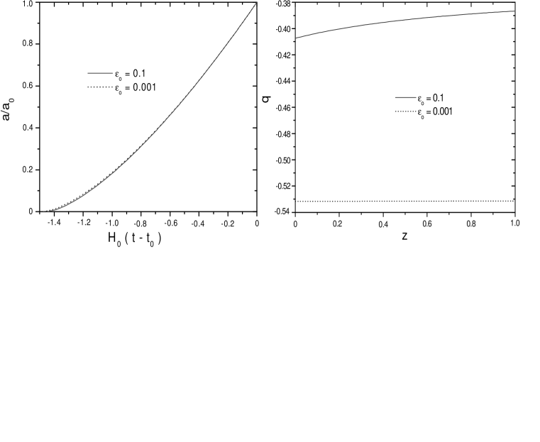
Figure 6: The left panel shows the scalar factor as a function of cosmological time. The right panel shows the deceleration parameter $q$ as a function of the redshift $z=x^{-1}-1$. In both cases $w_{0}$=-0.9, $w_{1}$=0.002, $r_{0}=3/7$ and $\alpha$=-0.2.

As Fig. 7 shows the model fits the supernova data points not less well than the concordance $\Lambda$CDM model does. The likelihood contours, Figs. 8 and 9, were calculated with the method of Markov’s chains. We used the prior $\Omega_{m}+\Omega_{\varphi}=1$ and that the parameters $w_{0}$ and $w_{1}$ are restricted by the condition that the value of the right hand side of Eq. (41) must lay in the interval $[-1,-1/3)$. The mean values of the parameters are: $\Omega_{\varphi}=0.246$, $w_{0}=-0.773$, $w_{1}=0.22$, $\varepsilon_{0}=0.0087$, $\alpha=-0.76$. Here, $\varepsilon_{0}$ is not so weakly constrained by the supernovae data as in the quintessence model. The present model predicts a mild evolution of the equation of state parameter with redshift. This is slightly at variance with the findings of Jassal et al. Jassal , but agrees with the model independent analysis of Alam et al. alam .

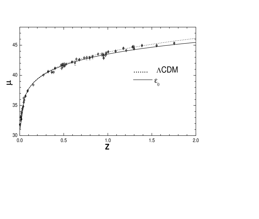
Figure 7: Distance moduli vs redshift for the tachyon–dark matter interacting model. In plotting the graphs the expression $\mu=5\log d_{L}+25$, with $d_{L}=(1+z)\int^{z}_{0}H^{-1}(z^{\prime})dz^{\prime}$ in units of megaparsecs was assumed. We have taken the values of the best fit model, namely: $w_{0}=-0.99$, $w_{1}=0.95$, $\varepsilon_{0}=0.0042$, $\alpha=-0.98$ and $r_{0}=0.136$. For comparison we have also plotted the prediction of the concordance $\Lambda$CDM model with $\Omega_{m0}=0.3$. The data points correspond to the “gold” sample of type Ia supernovae of Ref. adam .

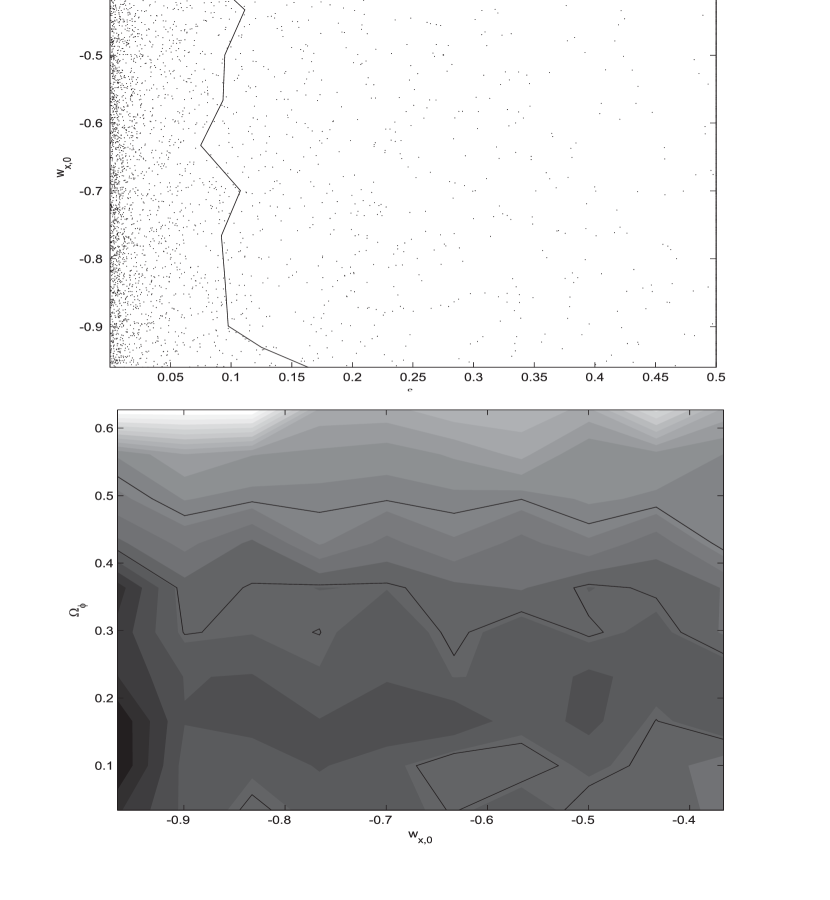
Figure 8: Likelihood contours for the tachyon–matter interacting model ($w_{x,0}$ vs. $\epsilon_{0}$ -top panel-, and $\Omega_{\varphi}$ vs. $w_{x,0}$, bottom panel) showing the 68% and 98% confidence intervals. The likelihoods are marginalized over the rest of parameters.

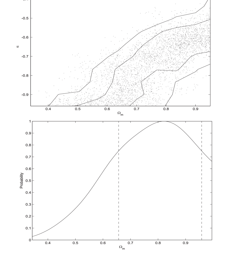
Figure 9: Top panel: likelihood contours for the tachyon–matter interacting model ($\alpha$ vs. $\Omega_{m})$) showing the 68% and 98% confidence intervals. Bottom panel: probability function of the matter density parameter. The likelihoods are marginalized over the rest of parameters.

The interaction term is given by

$$Q(x)=Q_{0}\,\frac{(1+r_{0})^{\frac{9\beta_{1}-1}{2}}}{[3r_{0}(\alpha-w_{0})-\varepsilon_{0}]}\left\{3[\alpha-w_{0}-w_{1}(1-x)][r_{0}+\varepsilon_{0}(1-x)]-\varepsilon_{0}x\right\}$$

$$\times\,\,x^{\frac{-9\beta_{2}}{2}}\left\{1+r_{0}+\varepsilon_{0}(1-x)\right\}^{\frac{1-9\beta_{1}}{2}}\,,$$ (49)

with $Q_{0}=\textstyle{1\over{2}}\rho_{\varphi}^{(0)}\,H_{0}[3r_{0}(\alpha-w_{0})-\varepsilon_{0}]$.
Likewise, the tachyon field and the potential are found to be

$$\varphi(x)=\varphi_{0}+\frac{(1+r_{0})^{\frac{1-3\beta_{1}}{2}}}{H_{0}}\int_{1}^{x}x^{\prime\frac{3\beta_{2}}{2}-1}\sqrt{1+w_{0}+w_{1}(1-x^{\prime})}(1+r_{0}+\varepsilon_{0}(1-x^{\prime}))^{\frac{3\beta_{1}-1}{2}}dx^{\prime}$$ (50)

and

$$V(x)=\rho_{\varphi}^{(0)}(1+r_{0})^{3\beta_{1}}\sqrt{-w_{0}-w_{1}(1-x)}\,x^{-3\beta_{2}}[1+r_{0}+\varepsilon_{0}(1-x)]^{-3\beta_{1}}\,,$$ (51)

respectively -see Fig. 10.

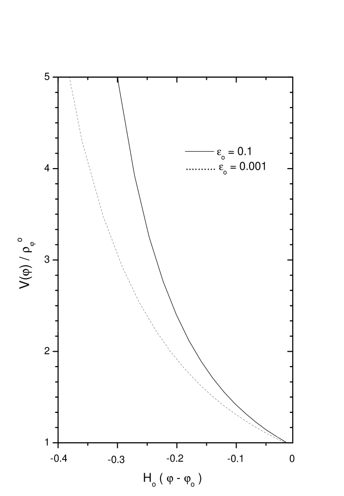
Figure 10: The effective potential as a function of the tachyonic field. Again, $w_{0}$=-0.9, $w_{1}$= 0.002, $r_{0}=3/7$ and $\alpha$= - 0.2.

IV Concluding remarks

We have studied two models of late acceleration by assuming $(i)$ that dark energy and non-relativistic dark matter do not conserve separately but the former decays into the latter as the Universe expands, and $(ii)$ that the present ratio of the dark matter density to dark energy density varies slowly with time, i.e., $\mid\dot{r}\mid_{0}\,\leq H_{0}$. This second assumption is key to determine the interaction $Q$ between both components.

In the quintessence model (section II) we have considered the equation of state parameter constant while in the tachyon field model (section III) we have allowed it to vary slightly. Actually, there is no compelling reason to impose that this parameter should be a constant. However, Jassal et al. Jassal have pointed out that the WMAP data spergel imply that in any case it cannot vary much. By contrast, Alam et al. using the sample of “gold” supernovae of Riess et al. adam find a clear evolution of $w$ in the redshift interval $0\leq z\leq 1$; however when strong priors on $\Omega_{m0}$ and $H_{0}$ are imposed this result weakens. Nevertheless, the analysis of these two papers assume that the two main components (matter and dark energy) do not interact with each other except gravitationally. The parameter $w_{0}$ presents degeneration in both models, therefore we must wait for further and more accurate SNIa data, perhaps from the future SNAP satellite, or to resort to complementary observations of the CMB.

In both cases (quintessence and tachyon), we have found analytical expressions for the relevant quantities (i.e., the scale factor, the field and the potential) and the solutions are seen to successfully pass the magnitude-redshift supernovae test -see Figs. 1 and 7. Nevertheless, it is apparent that the the tachyon model favors rather high values of the matter density parameter (see bottom right panel of Fig. 8) which is at variance with a variety of measurements of matter abundance at cosmic scales peebles which, taken as a whole, hint that $\Omega_{m}$ should not exceed $\sim 0.45$. In consequence, the quintessence model appears favored over the tachyon model. Our work may serve to build more sophisticated models aimed to simultaneously account for the present acceleration and the coincidence problem.

Previous studies of interacting dark energy aimed to solve the coincidence problem by demanding that the ratio $r$ be strictly constant at late times needed to prove the stability of $r$ at such times. This was achieved by showing that the models satisfied an attractor condition that involved the equation of state parameter of matter and dark energy as well as the Hubble factor and its temporal derivative plb ; interacting ; dw . Since in the case at hand the coincidence problem is solved with a (slowly) varying ratio $r$ no stability proof is necessary at all and no attractor condition is needed.

Our analysis was confined to times not far from the present (i.e., for $x\sim{\cal O}(1)$. To recover the evolution of the Universe at earlier times ($x\ll 1$), when the matter density dominated and produced via gravitational instability the cosmic structures we observe today, we must generalize our study along the lines of Refs. interacting and dw and include the baryon component in the dynamic equations as an uncoupled fluid.

We restricted ourselves to scenarios satisfying $w>-1$. Scenarios with $w<-1$ (the so-called “phantom” energy models) violate the dominant energy condition though, nevertheless, they are observationally favored rather than excluded alessandro and exhibit interesting features caldwell that might call for “new physics”. We defer the study of phantom models presenting soft coincidence to a future publication.