Evaluation of Cosmic Ray Rejection Algorithms on Single-shot Exposures

1 Introduction

Telescope observations suffer from the isotropic influx of (hadronic) cosmic rays striking their charge coupled device (CCD) detectors. In imaging these cosmic rays manifest as features with highly significant power at spatial frequencies ($\sim$one–several pixels) too high to be considered as legitimate objects (Rhoads 2000). Although there exist some uses for such cosmic rays (e.g. Pimbblet & Bulmer (2005) use cosmic rays in the generation of random numbers), generally one will want to detect and remove them.

Cosmic rays accumulate linearly in time on a detector and significant numbers are accumulated on an image or spectrum during longer exposures. Particularly when obtained in the higher radiation environment in orbit or outside the Earth’s magnetic field, images may suffer extensive data loss. For example, Offenberg et al. (1999) predict that up to 10 per cent of the Next Generation Space Telescope field of view may be affected by cosmic rays during a 1000s exposure. Efficient mechanisms for detecting and removing such defects are a vital consideration.

There are a plethora of approaches to the problem of cosmic ray rejection (CRR herein). The most frequently used solution is to have multiple images of the same astronomical target: cosmic rays are very unlikely to hit the same pixel more than once in a series of exposures. The images in which the cosmic rays are not present are then used to compute a replacement value (Shaw & Horne 1992; Windhorst, Franklin & Neuschaefer 1994; Zhang 1995; Freudling 1995; Fruchter & Hook 1997).

A tougher CRR problem arises in the case of single-shot exposures (e.g. for fast moving targets; time-critical observations or data processing; or where multiple images are simply unavailable; Pimbblet & Drinkwater 2004). In these instances image processing techniques must exploit the intrinsic properties of CCD cosmic ray events: their sharpness and high power at high spatial frequency. A number of methods have been developed to identify and replace pixels affected by cosmic rays in both imaging and spectroscopic data. Some of these include median or mean filtering (e.g. Dickinson’s IRAF tasks qzap, xzap and xnzap; http://www.starlink.ac.uk/iraf/ftp/iraf/extern-v212/xdimsum/xdimsum.readme), applying a threshold on the contrast of high intensity objects with surrounding pixels (e.g. IRAF task cosmicrays), convolution with specially designed adaptations of a point-spread function (PSF; Rhoads 2000), Laplacian edge detection (van Dokkum 2001), trainable classification of objects in an image (Murtagh 1992; Salzberg et al. 1995; SExtractor by Bertin & Arnouts, 1996) and analysis of the image data histogram (Pych 2004).

In implementing such a process, a maximum possible number of cosmic rays should be detected, flagged and ‘cleaned’ (replaced by a reasonable interpolated pixel value). Coincidently, the method must minimise the number of non-cosmic ray pixels that are falsely flagged to prevent loss of useful data.

This work presents an investigation into the performance of several CRR techniques for single-shot astronomical image processing. The primary aims are to make a comparison of the selected techniques and to examine their performance under different conditions. In Section 2 we present the rejection algorithms, details of the real and artificial datasets to which they are applied and the measures of performance used. The results of the tests are presented in Section 3, followed by a discussion of the results and the subsequent conclusions of the study in Section 4.

2 Evaluation

2.1 Algorithms

Of the available cosmic ray detection and rejection algorithms, the following four commonly used methods were selected for testing (identified by the developer and algorithm name): Rhoads’ (2000) IRAF script, jcrrej2; van Dokkum’s (2001) IRAF script, L.A.Cosmic; Pych’s (2004) C script, dcr; and Dickinson’s IRAF task, xzap (http://www.starlink.ac.uk/iraf/ftp/iraf/extern-v212/xdimsum/xdimsum.readme). All of these algorithms are idempotent: repeat usage of them produces no further effect. In implementing each algorithm, the user provides the input to a number of free parameters that customise the behaviour of the process. These must, by necessity, be adjusted experimentally to obtain the best detection and reconstruction for a given image. Here we briefly review the pertinent details of the selected algorithms and comment on the omission of several potential candidates.

Rhoads’ (2000) IRAF task implements a linear filtering process in which the free parameters are the image PSF and noise properties, the upper sigma clipping threshold for cosmic ray identification and a choice of the algorithm used to replace flagged pixels. The process convolves the image with a function derived from the difference between a Gaussian PSF and a scaled delta function. Pixels constituting cosmic ray events are then identified as those with intensities lying above the threshold value. The algorithm performs multiple iterations of the process to ensure that pixels ‘shielded’ by cosmic ray neighbours in previous applications can detected. Rhoads (2000) indicates that the probability of the algorithm falsely flagging a pixel containing legitimate object flux as a cosmic ray will not exceed that for a blank sky pixel, in order to decrease the rejection of true data. This safety check is likely to cost some efficiency in rejecting cosmic rays on real objects. The point is also made that well sampled data with, in practice, a seeing of $\geq$ 2 pixels is required for successful operation of the algorithm (Rhoads 2000). The output of the algorithm is a cosmic ray mask image in which only the cosmic ray affected pixels are assigned non-zero flux values. The Rhoads’ method does not directly output a cleaned image from which the detected cosmic rays have been removed and are replaced. An independent algorithm is required in order to complete the cosmic ray rejection process (for example, the IRAF fixpix task), though this has not been performed in these tests of the capabilities of the cosmic ray rejection algorithms.

The L.A.Cosmic – Laplacian Cosmic Ray Identification – algorithm (van Dokkum 2001) relies on the sharpness of the edges of cosmic ray objects in the detection process. The free parameters are: a detection limit for cosmic rays in terms of the background standard deviation ($\sigma$), a criterion for the detection of neighbouring pixels and a contrast limit for discriminating between cosmic rays and other objects. Again, the process is iterative, and at each step makes an estimate of the image noise properties and gain (if not provided at the input), identifies cosmic ray pixels, differentiates between cosmic rays and objects and fixes the flagged pixels. When no further cosmic ray candidates are detected, the iterations halt and the cleaned image and a bad pixel map of the detected objects are output. The algorithm has been designed with the intention of application to potentially undersampled data from the Hubble Space Telescope (HST), and the author makes recommendations as to appropriate example settings for such images.

Pych (2004) takes a different approach to cosmic ray detection. Rather than using an image filtering or modeling technique, the algorithm makes an analysis of the histogram of counts in small sub-sections of the image. The free parameters include a threshold value, the size of the sub-frame box and details about the method of interpolation and replacement of flagged pixels. The user can also specify a growing radius within which pixels surrounding those flagged as cosmic rays should also be flagged. Cosmic ray objects in an image exhibit a non-Gaussian profile and therefore affect the local image statistics, causing a deviation from the expected Gaussian distribution of counts. The algorithm examines the histogram for anomalous high-count points that are separated by more than the given threshold from the main distribution. The program creates a cosmic ray map and cleaned image after a specified number of iterations of the detection and replacement process. We note that Pych (2004) recommends the method as most appropriate for spectroscopic data, and less effective than other methods, such as those of Rhoads (2000) and van Dokkum (2001), in the case of images with a narrow PSF.

The final technique examined is the IRAF xzap task by Dickinson, a component of the IRAF xdimsum package. Unlike the other algorithms, this method is non-iterative, applying a spatial median filter to the image to perform an unsharp masking process and flagging pixels above a supplied threshold in a single detection step. The task will detect the background sky standard deviation, though the process requires manual examination of the image and identification and input of a section of the images that contains only sky background and is free of objects and cosmic rays. Other free parameters when applying the task to an image are the median filter box size, the cosmic ray object ‘zapping’ threshold, the threshold value for object identification and the cutoff for sky pixel rejection. Several parameters are also available to cause pixels surrounding detected cosmic rays to be flagged in addition, and for setting pixels surrounding objects as a buffer around the object. A map of the detected cosmic rays and a cleaned image are produced.

It is worth mentioning several other CRR algorithms that, though perhaps accessible, were omitted from the study. The IRAF task cosmicrays (Wells & Bell, http://star-www.rl.ac.uk/iraf/ftp/iraf/docs/clean.ps.Z) of the ccdred package detects pixels above a specified threshold and flags them as cosmic rays if they match a flux ratio criteria relative to surrounding pixels. Effective application of the process is time-consuming, requiring either an interactive examination process to determine the appropriate flux ratio, or prior identification and input of the nature and location of a sample of image objects so that the parameter can be determined automatically. In initial testing, the performance of this algorithm did not match that of the other candidate processes closely enough to warrant more rigorous assessment. Pych (2004) also notes its poor performance relative to his own algorithm and an inability to remove multiple pixel cosmic ray events.
Trainable classifier methods have also been omitted from the study, because the reliance on a training set adds an element of subjectivity in its selection, and requires time to obtain. xnzap (http://www.starlink.ac.uk/iraf/ftp/iraf/extern-v212/xdimsum/xdimsum.readme) is another method included in the IRAF xdimsum package. It operates very similarly to xzap, but utilises an averaging filter rather than a median filter. It was decided to select only one of the two tasks for testing, and the choice was dictated largely by the greater popularity of the median filtering method and the results of preliminary tests.
Discriminating use of the SExtractor package (Bertin & Arnouts 1996) is another conceivable means of detecting cosmic rays. SExtractor builds a catalogue of objects in an image, selecting candidates based on a set of detection criteria such as a threshold intensity, area on the CCD, and various deblending properties. Whilst promising, developing the required technique is outside the scope of this study.

2.2 Mock data

In order to equitably compare the selected CRR methods the IRAF artdata package is used to generate a controlled dataset of artificial images. Stars and galaxies are simulated with the starlist and gallist tasks, respectively, the images are compiled with mkobjects, and mknoise is used to add noise and cosmic rays events (of various ‘morphologies’). The simulated images are 2048x2048 pixels in size, with Poisson noise added to an average background of 1000 counts, producing a standard deviation in the background of 22.5 counts. Each image has a gain of 2, a 5 electron read noise and FWHM of seeing of 4 pixels. The cosmic ray objects are first combined with galaxy and/or star objects in the datasets and other noise properties are added as the last step in creating an image. mknoise generates cosmic ray objects in an image with an elliptical Gaussian profile defined by the following input parameters: a random intensity (with a maximum of 30000 counts in our images), the radius at FWHM (in pixels), the minor to major axial ratio, and the position angle. The cosmic rays are added iteratively, varying the input parameters, in order to generate a realistic range of cosmic ray shapes, sizes and orientations. Appropriate combinations of the cosmic ray morphology parameters are generated by selecting the geometric value for each event randomly from one of the categories in Table 1. In each image to which cosmic rays are added, the frequency of events from categories 1, 2 and 3 is in the ratio 2:1:1 respectively (derived from an inspection of cosmic ray events in our real data). Each cosmic ray is oriented with a random position angle between 1^∘ and 180^∘.

Table 1: The radius and axial ratio for the 3 categories of cosmic rays added to the artificial images.

Category	Radius range	Axial ratio range
	(pixels)
1 (small)	0.4 – 1.0	0.01 – 1.00
2 (non-elongated)	1.00 – 2.00	0.10 – 0.40
3 (elongated)	2.0 – 5.0	0.005 – 0.100

2.2.1 Test Methods

We identify two independent image properties that are relevant to the investigation of CRR techniques and with which we can describe a particular astronomical image:

1. the density of real (non-noise) objects in the field; and

2. the frequency of cosmic ray affected pixels.

Evidently, the CRR task should become more difficult as either of these properties increase and provide greater opportunity for intersection between cosmic rays and objects and loss of data to impinging cosmic rays. A qualitative measure of the former attribute is used in developing the mock dataset. Three images are created that exemplify three distinct and disparate degrees of object density as shown in Figure 1. The first, Figure 1(a), is the trivial case of an image consisting simply of a uniform noise background, the second, Figure 1(b), a field containing a number of sparse stellar and galactic objects and the third, Figure 1(c), an extremely crowded image containing a large globular star cluster.

(a) Poisson noise background: empty field

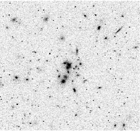
(b) Intermediate object density: sparse galactic and stellar field

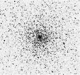
(c) High object density: globular star cluster

Figure 1: Central sections of the mock images demonstrating three degrees of object density.

The frequency of cosmic ray events is quantified using a cosmic ray ‘filling factor’. This is defined as the percentage of image pixels that are part of a cosmic ray event. For the simulated cosmic rays, such pixels are defined to be those that, after embedding the cosmic ray image in a noise background, have an intensity $\geq 4\sigma$ above the mean background level. Eleven levels (see Table 2) of cosmic ray filling factor are used in combination with the three base images to create an overall set of 33 images. For each level, a known number of cosmic ray objects are added to the images to create an approximately even distribution of filling factors. The SExtractor package (Bertin & Arnouts 1996) is used to catalogue the number of cosmic ray objects that are then present in each image, since the addition of Poisson noise obscures the weaker and smaller cosmic rays added. A mask image is created for each level indicating the location of all cosmic ray affected pixels (with intensity $\geq 4\sigma$ and excluding ‘hot’ background pixels). The number of cosmic ray pixels can then be counted and expressed as a percentage of the total image pixels to give the cosmic ray filling factor for each level, as shown in Table 2. The dependance of the final value on the random distribution and morphologies of the events prevents us arbitrarily selecting evenly spread, round numbers for the filling factor variable.

Table 2: Cosmic ray filling factor levels used in mock data trials.

Filling factor	N(cosmic rays)
(per cent)
0.06	233
0.12	463
0.24	918
0.37	1357
0.49	1801
0.61	2232
0.73	2675
0.86	3117
0.98	3550
1.10	3986
1.22	4412

Selecting the optimal settings of the free parameters for a given method of CRR in an image is a compromise between maximising the cosmic ray detections, minimising the number of false detections and ensuring a satisfactory cleaning of the image. Ideally, it would be preferable to experiment iteratively with the settings of an algorithm for each cosmic ray-affected image, to determine the combination of parameters that produces results of the quality required for an intended application. This is a prohibitively time consuming process, in the case of a time series analysis, where a large number of images need to be processed. In this investigation however, given prior knowledge of the details of the cosmic rays in the image and to provide a fair comparison of the methods tested, experimentation is extensive. The CRR procedures are repeatedly applied to a selected artificial image of intermediate object density (Figure 1(b)) and $\sim$0.7 per cent filling factor (Table 2), as the relevant task inputs are iteratively varied. The detection pixel map produced in each instance is examined to determine the number of flagged pixels known to be true cosmic rays and, as a result, the number of falsely flagged pixels. The process is defined to be ‘optimised’ (at least for this image) by the parameter set resulting in the maximum number of genuine cosmic ray pixel detections with a false detection rate of less than 0.01 per cent. The appropriate parameter set for each algorithm is then used to process each image of the mock dataset and the outcomes are used as the basis for comparison of the performance of the processes. In this way we impose a consistent standard on each algorithm and evaluate at a similar level of performance across the dataset, under the assumption that similar noise properties among the images will ensure reasonable results in each case.

For those algorithms that produce a cleaned version of the image, another important aspect of the performance is the quality of this image reconstruction. Explicitly, we are concerned with how well the value of flagged cosmic ray pixels are interpolated from the real data, the degree to which cleaning of false detections affects the image data and whether artifacts of the cleaning process can be observed in the output image.

2.3 Real data

The capabilities of the algorithms are also evaluated using a real image that contains true cosmic rays incurred during the exposure. The observation was made with the Wide Field Imager (WFI) on the Anglo-Australia Telescope, which consists of an 8k x 8k array of 8 CCD panels. The mosaic image that is the subject of tests contains sparse stellar and galactic objects and a significant sample of true cosmic rays. The FWHM of seeing is 5.3 pixels. In addition to the genuine noise events present, a sample of artificial cosmic rays is added to the images and the CRR performance is assessed by a blind test. The success of detection and removal of the simulated cosmic rays is taken to be indicative of the efficiency of real cosmic ray removal. 600 events with morphologies similar to that described in Section 2.2 above are added randomly across the image, and a cosmic ray map is created of all pixels affected by the artificial cosmic rays so that detections of artificial objects can be examined. Cosmic ray pixels are again defined as those containing flux $\geq 4\sigma$ above the mean background level. These tests are more qualitatively conducted than the artificial image testing presented in the previous section. The algorithms are applied several times to each image, making manual adjustments to the free parameters in an attempt to customise the process to the image. The best result is selected by visual inspection of the output.

3 Results

3.1 Mock Data

Using various manipulations of the output images (cosmic ray maps and cleaned images) with the artificial cosmic ray mask images, it is possible to quantify the following properties of the results for each subject image:

1. The number of true cosmic ray pixels that are detected; and

2. The number of pixels that are falsely flagged as cosmic rays (e.g. pixels containing only object or improbably high background flux).

The value of (i) is taken to be the best indicator of the efficiency of detection of cosmic ray events. The results are expressed as the fraction of the total number of cosmic ray pixels in the original image (those contributing to the image filling factor). Figure 2 presents the detection efficiency results from the mock data trials decribed in Section 2.2, for the four algorithms as a function of the cosmic ray filling factor.

(a) Detection efficiencies of the Rhoads (2000) and xzap algorithms.

(b) Detection efficiencies of the Pych (2004) and van Dokkum (2001) algorithms.

Figure 2: Cosmic ray pixel detection efficiency results. For images of similar object density, the effiency of detection is independent of the cosmic ray filling factor, though reduced by increasing object density. Poisson errors are indicated as a median error magnitude.

The false detections made during the CRR process, (ii), represent real data that is altered by the algorithm. We wish to minimise this data loss, of which we would generally be unaware of unless the results are thoroughly examined by eye. Figure 3 shows the numbers of spurious detections made by the algorithms during the testing of simulated images. These results, as a function of the filling factor, are presented individually for the different algorithms such that the effect of image properties can be more clearly observed. It is seen that comparable levels of false detections are made amongst the test subjects, with the exception of the Pych algorithm in the high object density limit.

(a) van Dokkum algorithm

(b) Pych algorithm

(c) Rhoads algorithm

(d) xzap algorithm

Figure 3: The number of spurious detections made by each algorithm as a function of filling factor, with simple Poissonian errors. Unlike the detection efficiency, the rate of false detections appear to have some dependency on the cosmic ray density for all other than Pych’s algorithm. The adverse effect of increasing object density is again demonstrated in these results.

3.2 Verification

The efficiency and false detection results can be confirmed using the reconstructed clean image if one is output by the algorithm. Of those tested, the van Dokkum, Pych and xzap algorithms produce a cleaned image as direct output so that assessment of the quality of cleaning is applicable. Analysis of the cleaned image confirms that the van Dokkum and Pych processes clean only those pixels that are flagged; that is, the number original image pixels that are altered is equal to the number of pixels indicated as detections in the output cosmic ray map. The Pych algorithm provides an option to flag pixels surrounding detections (and hence clean them), however these options are not utilised in order to avoid the resulting spurious detections that would be associated with the cosmic ray events. Notably, the xzap task is found to clean more pixels than are flagged, although again, the parameters that specify neighbouring pixels to be flagged or altered have not been applied. Thus, more of the actual cosmic ray pixels are altered and the ‘cleaning efficiency’ is approximately 2 percentage points higher than is indicated by the detection efficiencies of Figure 3(d). Examining the reconstructed images also then reveals a greater number of false detections surrounding detected cosmic ray pixels.

3.3 Real Data

The results of the blind tests on the real data appear in Table 3. These are the best results that could be obtained with limited experimentation. The large image size brought to notice the issue of time constraints, and here the Pych and xzap processes gain some advantage in requiring far less operating time than either the Rhoads or van Dokkum algorithms, which are relatively computationally expensive. The van Dokkum algorithm, however, clearly produces the best detection performance. This is in contrast to the mock data results. We consider that there may be an over abundance of larger cosmic ray events in our mock data. We suggest that this contributes to decreased performance of the van Dokkum algorithm on the mock data, since it is observed that events missed by this method are generally the largest cosmic ray events present.

Table 3: The best fractional cosmic ray efficiencies achieved for the real data set. Errors are simple Poissonian errors.

CRR Method	N(detections)	Error	Efficiency	Error
	(pixels)	(pixels)
van Dokkum	5969	77	0.86	0.015
Rhoads	5410	74	0.78	0.014
Xzap	5405	74	0.78	0.014
Pych	5267	73	0.76	0.014

4 Discussion and Conclusions

It is interesting to note that the filling factor appears to have little or no effect on the performance of cosmic ray detection (Figure 2). Only the Pych results show even a noticeable drop in the efficiency of detection with increasing filling factor,in the range of values tested. This is contrary to our intuitive prediction that the detection efficiency would be significantly affected by the larger numbers of intersecting events as the filling factor is increased. Also from Figure 2 the image object density is of greater importance, causing significant reductions in performance as it is increased. This is most noticable in the results from the Rhoads algorithm, which are markedly better for the empty, noise image. As would be expected, it is also clearly illustrated by the effects on the rate of spurious detections; in particular by the Pych algorithm results (Figure 3), which exhibit a dramatic increase in false detections in the most dense image field where there is a much larger number of candidate objects for false dectection.

In terms of detection, the algorithms do not perform as well as expected in the tests of the empty, noise image. It is presumed that a much better result would be obtained for the trivial case by determining the optimising parameter set using the empty image, eliminating the need for the algorithm to distinguish between objects and cosmic rays.

The false detection rates, with the exception of the results from Pych’s algorithm, appear to exhibit some dependence on the filling factor, in addition to being affected by the object density. Unlike the effects of increasing the object density which, in providing more objects that could potentially be falsely flagged as cosmic rays, might be expected, the increase in false detections with filling factor is unexpected and counter-intuitive. It is explained, however, by comparison of false detection image maps from each algorithm with the original cosmic ray maps created for addition to the simulated images, prior to the addition of background noise and imposing the definition of cosmic rays as objects with intensities $\geq 4\sigma$. It is clear the vast majority of false detections made by the van Dokkum and Rhoads algorithm and most of those made by the xzap algorithm are sub-threshold simulated cosmic rays or pixels at the edges of simulated cosmic rays. These pixels are then not true false detections, but instances where the addition of noise to the image with added cosmic rays has ’smeared’ the edges and low-intesity cosmic rays to below the subsequently defined cosmic ray threshold. The Pych algorithm results do not exhibit the same detection of sub-threshold cosmic rays and so the results in Figure 3(b) show no filling factor dependency. In hindsight, a more successful method would remove subthreshold pixels from cosmic ray before adding them to the artificial images. An indication of the numbers of false detections made by the van Dokkum, Rhoads and xzap algorithms can be better derived from the values detected at very low filling factors.

The quality of the image cleaning is best illustrated by example, since it is somewhat objective and is largely judged by the visual appearance. Figure 4 compares a portion of the test image, of intermediate object and cosmic ray density, and the reconstructed image output by the three algorithms that produce a cleaned image. The original image, prior to cosmic ray addition, is at top in Figure 4(a), with the true cosmic ray image beneath. Figures 4(b), 4(c) and 4(d) show the cleaned output image above and the detected cosmic ray map below from the van Dokkum, Pych and xzap algorithms, respectively.

(a) Original image

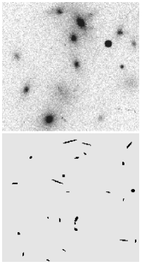
(b) van Dokkum algorithm

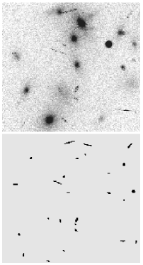
(c) Pych algorithm

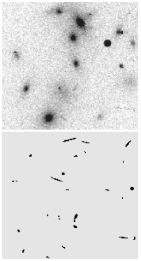
(d) xzap algorithm

Figure 4: A sample of resulting cleaned and cosmic ray map image sections for the artifical image that is used to optimise the algorithm performance in the tests.

From general observations of the results obtained throughout the study, the van Dokkum algorithm produces a very well-cleaned image, though the algorithm tends sometimes to miss detecting the relatively larger and less elongated cosmic ray events. The cleaned output of the xzap algorithm is also impressive in many cases, though the use of a small median filter box (to reduce detections of true objects) can cause only sections of cosmic rays to be detected, and hence some remnant to remain in the image. Though the Rhoads algorithm does not directly output a cleaned image, the algorithm sets the highest standard of detection in the mock data trials, and performs well on the real data tested. Pych’s (2004) advice that his algorithm is designed for spectroscopic, rather than imaging, data should perhaps be heeded, as the alorithm’s performance on the imaging data tested was certainly not equal to that of the others. However, it must be emphasised that since no comparative testing has been performed on spectroscopic data, and the Pych algorithm performance may well exceed that of other methods here. The analysis of the image in small subframes often produces spurious detections of objects at the frame edges and sometimes leaves artifacts in the image, such as anomolous alteration of data at the edges or outer regions of multiple-pixel cosmic rays. All the algorithms make spurious detections at regions of overexposure on the CCD, and at regions of non-uniformity in the background flat-fielding, such as striations where the mean background levels are significantly altered to higher intensities.

In conclusion, the primary findings of the investigation are summarised below:

1. The cosmic ray detection efficiencies and false detection rates of the CRR algorithms tested are independent of the density of cosmic ray events in an image (in the range of ‘filling factors’ tested), but are affected by the density of true objects native to the field observed.

2. From the mock data trials, Rhoads’ detection algorithm exhibits the highest cosmic ray detection efficiency of those tested, and exhibits a reasonable (less than 0.02 per cent) false detection rate in mock data trials. It is followed closely by the van Dokkum algorithm, which actually supercedes the results of Rhoads’ algorithm when applied to the real observational data sample described.

3. The van Dokkum algorithm produces the most satisfactory cleaned image as output, though it is a relatively slow process. The IRAF xzap algorithm provides a faster alternative, at a cost of a decrease in the quality of the result.

Further investigation and testing of both a more extensive set of images types (particularly to include spectroscopic data) and cosmic ray rejection methods would be prudent to elaborate on and extend the results presented here.

References

- Bertin & Arnouts (1996) Bertin E., Arnouts S., 1996, A&AS, 117, 393
- Freudling (1995) Freudling W., 1995, PASP, 107, 85
- Fruchter & Hook (1997) Fruchter A., Hook R. N., 1997, SPIE, 3164, 120
- Murtagh (1992) Murtagh F. D., 1992, ASPC, 25, 265
- Offenberg et al. (1999) Offenberg J. D., Sengupta R., Fixsen D. J., Stockman P., Nieto-Santisteban M., Stallcup S., Hanisch R., Mather J. C., 1999, ASPC, 172, 141
- Pimbblet & Bulmer (2005) Pimbblet K. A., Bulmer M., 2005, PASA, 22, 1
- Pimbblet & Drinkwater (2004) Pimbblet K. A., Drinkwater M. J., 2004, MNRAS, 347, 137
- Pych (2004) Pych W., 2004, PASP, 116, 148
- Rhoads (2000) Rhoads J. E., 2000, PASP, 112, 703
- Salzberg et al. (1995) Salzberg S., Chandar R., Ford H., Murthy S. K., White R., 1995, PASP, 107, 279
- Shaw & Horne (1992) Shaw R. A., Horne K., 1992, ASPC, 25, 311
- van Dokkum (2001) van Dokkum P. G., 2001, PASP, 113, 1420
- Windhorst, Franklin, & Neuschaefer (1994) Windhorst R. A., Franklin B. E., Neuschaefer L. W., 1994, PASP, 106, 798
- Zhang (1995) Zhang C. Y., 1995, ASPC, 77, 514