FADC Pulse Reconstruction Using a Digital Filter for the MAGIC Telescope

(a) Max-Planck-Institute for Physics, Munich, Germany
(b) Institut de Fisica d Altes Energies, Bellaterra, Spain
(c) University and INFN Padova, Italy

Presently, the MAGIC telescope uses a 300 MHz FADC system to sample the transmitted and shaped signals from the captured Cherenkov light of air showers. We describe a method of Digital Filtering of the FADC samples to extract the charge and the arrival time of the signal: Since the pulse shape is dominated by the electronic pulse shaper, a numerical fit can be applied to the FADC samples taking the noise autocorrelation into account. The achievable performance of the digital filter is presented and compared to other signal reconstruction algorithms.

1 Introduction

The purpose of the MAGIC Telescope [1] is the observation of high energy gamma radiation from celestial objects. When the gamma quanta hit the earth atmosphere they initiate a cascade of photons, electrons and positrons. The latter radiate short flashes of Cherenkov light which can be recorded by a Cherenkov telescope. The FWHM of the pulses is about 2 ns.

In order to sample this pulse shape with the 300 MSamples/s FADC system [2], the original pulse is folded with a stretching function leading to a FWHM greater than 6 ns. To increase the dynamic range of the MAGIC FADCs the signals are split into two branches with gains differing by a factor 10. Figure 1a) shows a typical average of identical signals.

In order to discriminate the small signals from showers in the energy range below 100 GeV against the light of the night sky (LONS) the highest possible signal to noise ratio, signal reconstruction resolution and a small bias are important.

Monte Carlo (MC) based simulations predict different time structures for gamma and hadron induced shower images as well as for images of single muons [7]. An accurate arrival time determination may therefore improve the separation power of gamma events from the background events. Moreover, the timing information may be used in the image cleaning to discriminate between pixels whose signal belongs to the shower and pixels which are dominated by randomly timed background noise.

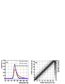
Figure 1: a) Average normalized reconstructed high and low gain pulse shapes and pulse shape implemented in the MC simulations [3]. b) Noise autocorrelation matrix $\boldsymbol{B}$ for open camera and averaged over all pixels (galactic telescope pointing).

2 Digital Filter

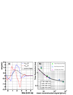
Figure 2: a) Amplitude weights $w_{\mathrm{amp}}(t_{0})\ldots w_{\mathrm{amp}}(t_{5})$ for a window size of 6 FADC slices for the pulse shape used in the MC simulations, see text. b) Timing resolution for calibration LED pulses [6].

The goal of the digital filtering method [4, 5] is to optimally reconstruct from FADC samples the amplitude and arrival time of a signal whose shape is known. Thereby, the noise contributions to the amplitude and arrival time reconstruction are minimized.

For the digital filtering method, three assumptions have to be made:

• The normalized signal shape has to be always constant.

• The noise properties must be constant, especially independent of the signal amplitude.

• The normalized noise auto-correlation has to be constant.

Due to the artificial pulse stretching by about 6 ns on the receiver board all three assumptions are fullfilled to a good approximation. For a more detailed discussion see [8].

Let $g(t)$ be the normalized signal shape, $E$ the signal amplitude and $\tau$ the time shift between the physical signal and the predicted signal shape. Then the time dependence of the signal, $y(t)$, is given by $y(t)=E\cdot g(t-\tau)+b(t)\ ,$ where $b(t)$ is the time-dependent noise contribution. For small time shifts $\tau$ (usually smaller than one FADC slice width), the time dependence can be linearized. Discrete measurements $y_{i}$ of the signal at times $t_{i}\ (i=1,...,n)$ have the form $y_{i}=E\cdot g_{i}-E\tau\cdot\dot{g}_{i}+O(\tau^{2})+b_{i}$, where $\dot{g}(t)$ is the time derivative of the signal shape.

The correlation of the noise contributions at times $t_{i}$ and $t_{j}$ can be expressed in the noise autocorrelation matrix $\boldsymbol{B}$: $B_{ij}=\langle b_{i}b_{j}\rangle-\langle b_{i}\rangle\langle b_{j}\rangle$. Figure 2 shows the noise autocorrelation matrix for an open camera. It is dominated by LONS pulses shaped to 6 ns.

The signal amplitude $E$, and the product $E\tau$ of amplitude and time shift, can be estimated from the given FADC measurements $\boldsymbol{y}=(y_{1},...,y_{n})$ by minimizing the deviation of the measured FADC slice contents from the known pulse shape with respect to the known noise auto-correlation: $\chi^{2}(E,E\tau)=(\boldsymbol{y}-E\boldsymbol{g}-E\tau\dot{\boldsymbol{g}})^{T}\boldsymbol{B}^{-1}(\boldsymbol{y}-E\boldsymbol{g}-E\tau\dot{\boldsymbol{g}})+O(\tau^{2})$ (in matrix form). This leads to the following solution for $\overline{E}$ and $\overline{E\tau}$:

$$\overline{E}=\boldsymbol{w}_{\text{amp}}^{T}(t_{\text{rel}})\boldsymbol{y}+O(\tau^{2})\quad\mathrm{with}\quad\boldsymbol{w}_{\text{amp}}(t_{\text{rel}})=\frac{(\dot{\boldsymbol{g}}^{T}\boldsymbol{B}^{-1}\dot{\boldsymbol{g}})\boldsymbol{B}^{-1}\boldsymbol{g}-(\boldsymbol{g}^{T}\boldsymbol{B}^{-1}\dot{\boldsymbol{g}})\boldsymbol{B}^{-1}\dot{\boldsymbol{g}}}{(\boldsymbol{g}^{T}\boldsymbol{B}^{-1}\boldsymbol{g})(\dot{\boldsymbol{g}}^{T}\boldsymbol{B}^{-1}\dot{\boldsymbol{g}})-(\dot{\boldsymbol{g}}^{T}\boldsymbol{B}^{-1}\boldsymbol{g})^{2}}\ ,$$ (1)

$$\overline{E\tau}=\boldsymbol{w}_{\text{time}}^{T}(t_{\text{rel}})\boldsymbol{y}+O(\tau^{2})\quad\mathrm{with}\quad\boldsymbol{w}_{\text{time}}(t_{\text{rel}})=\frac{({\boldsymbol{g}}^{T}\boldsymbol{B}^{-1}{\boldsymbol{g}})\boldsymbol{B}^{-1}\dot{\boldsymbol{g}}-(\boldsymbol{g}^{T}\boldsymbol{B}^{-1}\dot{\boldsymbol{g}})\boldsymbol{B}^{-1}{\boldsymbol{g}}}{(\boldsymbol{g}^{T}\boldsymbol{B}^{-1}\boldsymbol{g})(\dot{\boldsymbol{g}}^{T}\boldsymbol{B}^{-1}\dot{\boldsymbol{g}})-(\dot{\boldsymbol{g}}^{T}\boldsymbol{B}^{-1}\boldsymbol{g})^{2}}\ ,$$ (2)

where $t_{\text{rel}}$ is the relative phase between $g(t)$ and the FADC clock. Thus $\overline{E}$ and $\overline{E\tau}$ are given by a weighted sum of the discrete measurements $y_{i}$ with the weights for the amplitude, $w_{\text{amp}}(t_{\text{rel}})$, and time shift, $w_{\text{time}}(t_{\text{rel}})$, plus $O(\tau^{2})$. To reduce $O(\tau^{2})$ the fit can be iterated using $g(t_{1}=t-\tau)$ and the weights $w_{\mathrm{amp/time}}(t_{\text{rel}}+\tau)$ [4, 8]. Figure 2 a) shows the amplitude and timing weights for the MC pulse shape. The first weight $w_{\mathrm{amp/time}}(t_{0})$ is plotted as a function of $t_{\text{rel}}$ in the range $[-0.5,0.5[\ T_{\text{ADC}}$, the second weight in the range $[0.5,1.5[\ T_{\text{ADC}}$ and so on.

The expected contributions of the noise to the error of the estimated amplitude and timing only depend on the the shape $g(t)$, and the noise auto-correlation $B$. Analytic expressions can be found in references [4, 8].

3 Performance and Discussion

Figure 2b) shows the measured timing resolution for different calibration LED pulses as a function of the mean reconstructed pulse charge. For signals of 10 photo-electrons the timing resolution is as good as 700 ps, for very large signals a timing resolution of about 200 ps can be achieved.

Figure 3 shows the charge and arrival time resolution as a function of the input pulse height for MC simulations (no PMT time spread and no gain fluctuations) assuming an extra-galactic background for different signal extraction algorithms. The digital filter yields the best charge and timing resolution of the studied algorithms [8].

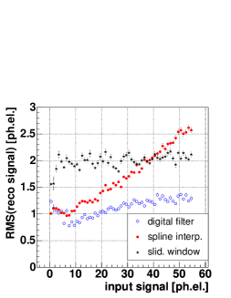
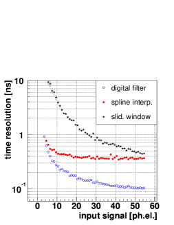
Figure 3: Charge and arrival time resolution as a function of the input pulse height for MC simulations for the Digital Filter, a cubic spline interpolation (charge= spline integral, time=half maximum position) and a sliding window of 6 FADC slices (charge=samples sum, time = pulse barycenter) [8].

For known constant signal shapes and noise auto-correlations the digital filter yields the best theoretically achievable signal and timing resolution. Due to the pulse shaping of the Cherenkov signals the algorithm can be applied to reconstruct their charge and arrival time, although there are some fluctuations of the pulse shape and noise behavior. The digital filter reduces the noise contribution to the error of the reconstructed signal. Thus it is possible to lower the image cleaning levels and the analysis energy threshold [8]. The timing resolutions is as good as a few hundred ps for large signals.

References

- [1] C. Baixeras et al. (MAGIC Collab.), Nucl. Instrum. Meth. A518 (2004) 188.
- [2] F. Goebel et al. (MAGIC Collab.), in Proceedings of the 28th ICRC, Tokyo, 2003.
- [3] A. Moralejo et al., MC Simulations for the MAGIC Telescope, In preparation.
- [4] W. E. Cleland and E. G. Stern, Nucl. Instrum. Meth. A338 (1994) 467.
- [5] A. Papoulis, Signal analysis, McGraw-Hill, 1977.
- [6] T. Schweizer et al., IEEE Trans. Nucl. Sci. 49 (2002) 2497.
- [7] R. Mirzoyan et al., to be published in proceedings of the conference Towards a Network of Atmospheric Cherenkov Detectors VII, 27-29 April 2005 Palaiseau, France.
- [8] H. Bartko et al., In preparation, to be submitted to Nucl. Inst. Meth.