The age of the Galactic thin disk from Th/Eu nucleocosmochronology

The first determination of the age of the Galactic thin disk from Th/Eu nucleocosmochronology was accomplished by us in Papers I and II. The present work aimed at reducing the age uncertainty by expanding the stellar sample with the inclusion of seven new objects – an increase by 37%. A set of [Th/Eu] abundance ratios was determined from spectral synthesis and merged with the results from Paper I. Abundances for the new, extended sample were analyzed with the aid of a Galactic disk chemical evolution (GDCE) model developed by us is Paper II. The result was averaged with an estimate obtained in Paper II from a conjunction of literature data and our GDCE model, providing our final, adopted disk age $T_{\mathrm{G}}=(8.8\pm 1.7)\leavevmode\nobreak\ \mbox{Gyr}$ with a reduction of 0.1 Gyr (6%) in the uncertainty. This value is compatible with the most up-to-date white dwarf age determinations ($\lesssim 10$ Gyr). Considering that the halo is currently presumed to be $(13.5\pm 0.7)\leavevmode\nobreak\ \mathrm{Gyr}$ old, our result prompts groups developing Galactic formation models to include an hiatus of $(4.7\pm 1.8)\leavevmode\nobreak\ \mathrm{Gyr}$ between the formation of halo and disk.

1 Introduction

The age of the Galactic thin disk is an important constraint for Galactic formation models. It is usually estimated by dating the oldest open clusters with isochrones or white dwarfs with cooling sequences. These methods are strongly dependent on stellar evolution models and on numerous physical parameters known at different levels of uncertainty. Nucleocosmochronology is only weakly dependent on main sequence stellar evolution models, allowing for a nearly independent crosscheck of other techniques.

We were the first to determine an age for the Galactic disk from Th/Eu nucleocosmochronology – del Peloso et al. 2005b (Paper I) and del Peloso et al. 2005a (Paper II), based on the PhD thesis of one of us (del Peloso 2003). This work, the last part in a series of three articles, aims at reducing the uncertainty in this determination by expanding the stellar sample from Papers I and II with objects observed only after the publication of del Peloso (2003) and deriving a new age from this extended sample. With this intent, we determined [Th/Eu] abundance ratios for a sample of Galactic disk stars and employed Galactic disk chemical evolution models developed by us in the chronological analysis.

2 Sample selection, observations and data reduction

Sample selection, observations and data reduction were carried out following exactly the same procedures described in detail in Paper I. In what follows we provide a brief overview of these topics.

The stellar sample of this work is composed of seven F8–G5 dwarfs and subgiants (Table 1). As the objective of this work is the determination of the age of the Galactic disk, we performed a kinematic analysis of the objects to help ensure that they do not belong to the Galactic halo. We calculated the objects’ $U$, $V$, and $W$ spatial velocity components (Table 2) and constructed a $V$ vs. [Fe/H] diagram (Figure 1) using metallicities from the literature (Table 3). According to Schuster et al. (1993), objects located above the displayed cut-off line belong to the Galactic halo, whereas those located below the line belong to the halo. It can be seen that all sample stars are located far above the cut-off line. For a star to cross the line, the literature metallicities would have to have been overestimated by at least 1.2 dex, which is very unlikely. After having determined our own metallicities (Table 4), we confirmed that results from the literature agree with our values to 0.1 dex.

Table 1: Selected stellar sample.

HD	HR	HIP	Name	R.A.	DEC	Parallax		V		Spectral type
				2000.0	2000.0	(mas)				and
				(h m s)	(d m s)					luminosity class
1461	72	1499	–	00 18 42	$-$08 03 11	42.	67	6.	46	G5 V
157 089	–	84 905	–	17 21 07	+01 26 35	25.	88	6.	95	G0–2 V
162 396	6649	87 523	–	17 52 53	$-$41 59 48	30.	55	6.	20	F8 IV–V
189 567	7644	98 959	–	20 05 33	$-$67 19 15	56.	45	6.	07	G3 V
193 307	7766	100 412	–	20 21 41	$-$49 59 58	30.	84	6.	27	G0 V
196 755	7896	101 916	$\kappa$ Del	20 39 08	+10 05 10	33.	27	5.	05	G5 IV
210 918	8477	109 821	–	22 14 39	$-$41 22 54	45.	19	6.	23	G5 V

References: Coordinates: SIMBAD (FK5 system); parallaxes: Hipparcos catalogue (Perryman & ESA 1997); visual magnitudes: Bright Star Catalogue (Warren & Hoffleit 1987) for stars with an HR number and SIMBAD for those without; spectral types and luminosity classes: Michigan Catalogue of HD Stars (Houk & Cowley 1975; Houk 1978; Houk & Swift 1999) for all stars, with the exception of HD 196 755 (Bright Star Catalogue).

Table 2: Radial velocities ($RV$) and spatial velocity components ($U$, $V$, and $W$) of the sample stars, in a right-handed Galactic system and relative to the LSR. All values are in km s^-1.

HD	$RV$		$U$		$V$		$W$
1461	$-$9.	3	$-$15.	3 $\pm$0.7	$-$36.	7 $\pm$1.0	+17.	0 $\pm$0.4
157 089	$-$161.	1	$-$156.	0 $\pm$1.1	$-$35.	5 $\pm$1.0	$-$2.	8 $\pm$1.8
162 396	$-$16.	4	$-$13.	3 $\pm$0.4	$-$5.	5 $\pm$0.7	$-$24.	0 $\pm$1.3
189 567	$-$10.	0	$-$59.	7 $\pm$1.6	$-$26.	4 $\pm$0.7	$-$42.	6 $\pm$2.0
193 307	+18.	6	+47.	4 $\pm$1.2	$-$43.	3 $\pm$1.6	+40.	8 $\pm$2.0
196 755	$-$52.	7	$-$48.	0 $\pm$0.8	$-$29.	5 $\pm$0.6	$-$11.	2 $\pm$1.0
210 918	$-$18.	6	$-$37.	4 $\pm$0.9	$-$86.	9 $\pm$1.6	$-$1.	8 $\pm$0.7

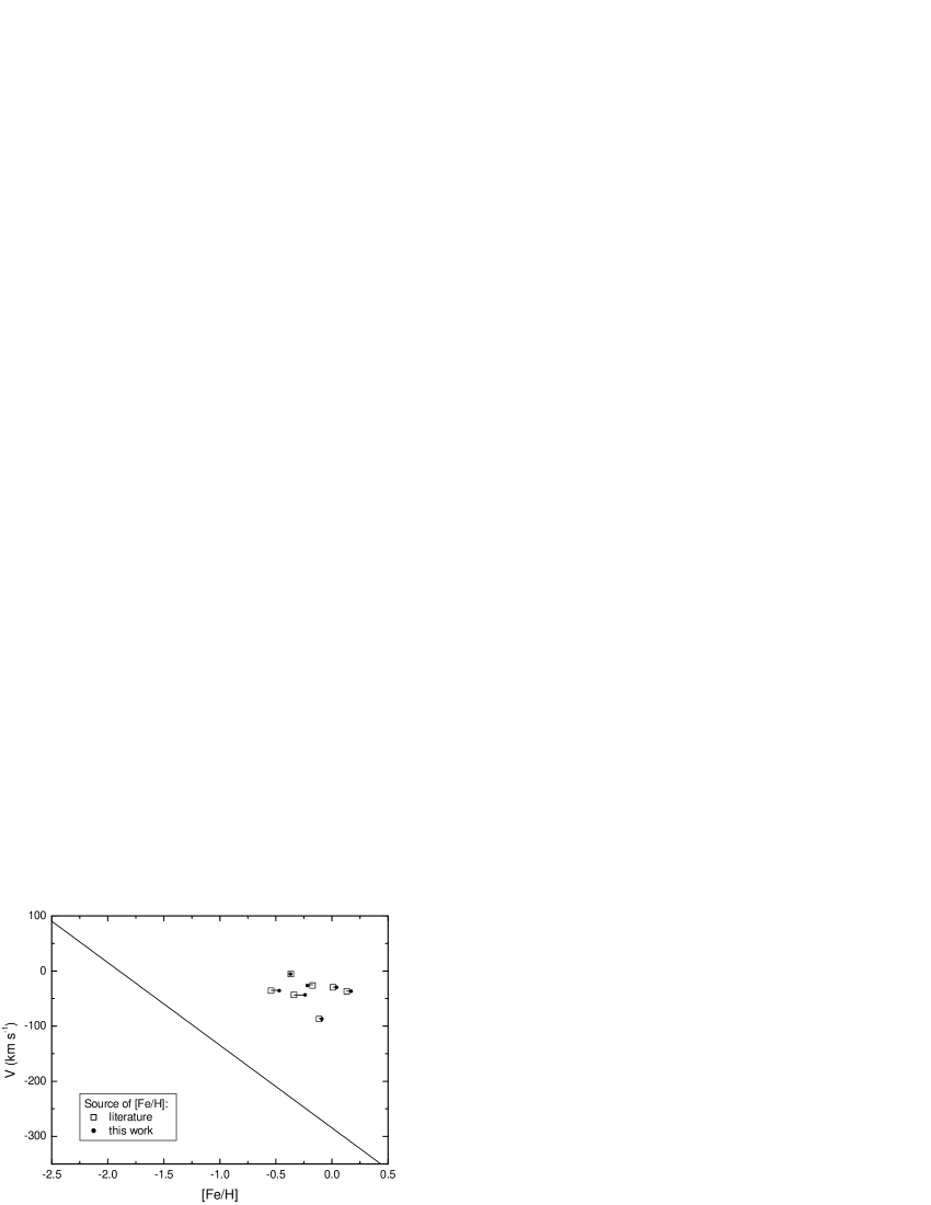
Figure 1: V vs. [Fe/H] diagram for the sample stars. The diagonal line is a cut off between the halo and the disk populations (below and above, respectively). Velocity components V were calculated by us. The metallicities initially employed, represented as open squares, were taken from the literature (Table 3); small filled circles represent metallicities derived in this work.

Table 3: Photometric indices and metallicities for all sample stars. Metallicities were taken from the literature for use in the kinematic characterization of the sample and as input for the first step in the iterative determination of atmospheric parameters.

HD	($B-V$)	Ref.	($b-y$)	Ref.	$\beta$	Ref.	($V-K$)	Ref.	($B_{\mathrm{T}}-V_{\mathrm{T}}$)	Ref.	$[$Fe/H$]$	Ref.
1461	0.68	1	0.422	3	2.596	4	1.518	7	0.764	9	+0.13	10
157 089	0.57	2	0.379	3	2.584	5	1.434	7	0.619	9	$-$0.54	11
162 396	0.54	1	0.347	4	2.612	4	–	–	0.563	9	$-$0.37	10
189 567	0.64	1	0.406	3	2.583	6	1.516	7	0.718	9	$-$0.17	10
193 307	0.55	1	0.365	3	2.604	5	–	–	0.617	9	$-$0.34	10
196 755	0.72	1	0.432	3	–	–	–	–	0.765	9	+0.01	10
210 918	0.65	1	0.404	3	2.590	6	1.500	8	–	9	$-$0.12	10

References: 1 - Warren & Hoffleit (1987); 2 - Mermilliod (1987); 3 - Olsen (1994); 4 - Grønbech & Olsen (1976, 1977); 5 - Olsen (1983); 6 - Schuster & Nissen (1988); 7 - di Benedetto (1998); 8 - Koornneef (1983); 9 - Perryman & ESA (1997); 10 - Taylor (2003); 11 - Cayrel de Strobel et al. (2001).

High resolution, high signal-to-noise ratio spectra were obtained for all objects with the Fiber-fed Extended Range Optical Spectrograph (FEROS;  Kaufer et al. 1999) fed by the 1.52 m European Southern Observatory (ESO) telescope, in the ESO-Observatório Nacional, Brazil, agreement (March and August 2001). Spectra were also obtained with a coudé spectrograph fed by the 1.60 m telescope of the Observatório do Pico dos Dias (OPD), LNA/MCT, Brazil (May and October 2000; May, August, and October 2002), and with the Coudé Échelle Spectrometer (CES) fiber-fed by ESO’s 3.60 m telescope (August 2003). FEROS spectra are reduced automatically during observation by a script executed using the European Southern Observatory Munich Image Data Analysis System (ESO-MIDAS) immediately after the CCD read out. OPD and CES spectra were reduced by us using the Image Reduction and Analysis Facility (IRAF), following the usual steps of bias, scattered light and flat field corrections, and extraction.

3 Atmospheric parameters

A set of homogeneous, self-consistent atmospheric parameters was determined for the sample stars, following the procedure described in detail in Paper I. Effective temperatures were derived from photometric calibrations (Table 3) and H$\alpha$ profile fitting; surface gravities were obtained from $T_{\mathrm{eff}}$, stellar masses and luminosities; microturbulence velocities and metallicities were obtained from detailed, differential spectroscopic analysis, relative to the Sun, using EWs of Fe i and Fe ii lines. The final, adopted values of all atmospheric parameters are presented in Table 4.

Table 4: Adopted atmospheric parameters, including the photometric and H$\alpha$ effective temperatures used to obtain the adopted mean values, and the stellar masses used to obtain the surface gravities.

HD	$T_{\mathrm{eff}}$ (K)				$m_{\mbox{\scriptsize\sun}}$	$\log g$	[Fe/H]	$\xi$ (km s-1)
	Phot.	H$\alpha$	MEAN
1461	5727	5705	5717		1.01	4.33	+0.17	1.20
157 089	5827	5742	5785		0.93	4.09	$-$0.47	0.90
162 396	6072	5979	6026		1.04	4.08	$-$0.37	1.36
189 567	5704	5715	5710		0.90	4.36	$-$0.22	1.01
193 307	5999	5956	5978		1.05	4.11	$-$0.24	1.25
196 755	5665	5613	5639		1.58	3.70	+0.04	1.42
210 918	5733	5708	5721		0.95	4.27	$-$0.09	1.15

4 Abundances of contaminating elements

Eu and Th abundances were determined by spectral synthesis of the Eu ii line at 4129.72 Å and of the Th ii line at 4019.13 Å, respectively. In the synthesis calculations, abundances of the elements that contaminate these spectral regions (Ti, V, Cr, Mn, Co, Ni, Ce, Nd, and Sm) were kept fixed in the values determined using EWs and the atmospheric parameters obtained by us; see Paper I for a full description of the employed method. Table 5 presents a sample of the EW data. Its complete content, composed of the EWs of all measured lines, for the Sun and all sample stars, is only available in electronic form at the CDS. Column 1 lists the central wavelength (in angstroms), Col. 2 gives the element symbol and degree of ionization, Col. 3 gives the excitation potential of the lower level of the electronic transition (in eV), Col. 4 presents the solar $\log gf$ derived by us, and the subsequent columns present the EWs, in mÅ, for the Sun and the other stars, from HD 1461 to HD 210 918.

Table 5: A sample of the EW data. The complete content of this table is only available in electronic form at the CDS. For a description of the columns, see text (Sect. 4).

$\lambda$ (Å)	Element	$\chi$ (eV)	$\log gf$	Sun	$\cdots$	HD 210 918
5668.362	V i	1.08	$-$0.920	8.5	$\cdots$	11.9
5670.851	V i	1.08	$-$0.452	21.6	$\cdots$	23.7
5727.661	V i	1.08	$-$0.657	9.5	$\cdots$	12.1
$\vdots$	$\vdots$	$\vdots$	$\vdots$	$\vdots$	$\vdots$	$\vdots$
5427.826	Fe ii	6.72	$-$1.371	6.4	$\cdots$	0.0
6149.249	Fe ii	3.89	$-$2.711	40.9	$\cdots$	39.5

Abundance results are presented in Table 6. No detailed uncertainty assessment was carried out. We have rather adopted an average of the uncertainties presented in Paper I: 0.08 dex for Mn, 0.09 dex for Fe, Ti, and Co, 0.10 dex for V, Cr, Ce, and Nd, and 0.11 dex for Ni and Sm. These values are used as error bars in Fig. 2, which shows the abundance patterns for all elements. Note that the abundances for the sample of this work (filled squares) agree very well with those from Paper I (open squares).

Table 6: Fe, Ti, V, Cr, Mn, Co, Ni, Ce, Nd, and Sm abundances, relative to H. N is the number of absorption lines effectively used for each abundance determination.

HD	[Fe i/H]	N	[Fe ii/H]	N	[Fe/H]	N	[Ti/H]	N	[V/H]	N	[Cr/H]	N	[Mn/H]	N
1461	+0.16	52	+0.19	8	+0.17	60	+0.16	28	+0.16	5	+0.18	19	+0.21	6
157 089	$-$0.47	31	$-$0.47	7	$-$0.47	38	$-$0.21	20	$-$0.21	3	$-$0.42	18	$-$0.66	4
162 396	$-$0.38	41	$-$0.33	8	$-$0.37	49	$-$0.29	18	$-$0.17	2	$-$0.35	16	$-$0.41	5
189 567	$-$0.23	44	$-$0.20	7	$-$0.22	51	$-$0.12	22	$-$0.10	3	$-$0.21	19	$-$0.29	6
193 307	$-$0.24	45	$-$0.22	9	$-$0.24	54	$-$0.21	19	$-$0.12	4	$-$0.21	19	$-$0.33	6
196 755	+0.04	45	+0.06	9	+0.04	54	+0.03	28	$-$0.01	5	+0.06	20	$-$0.01	6
210 918	$-$0.09	47	$-$0.09	7	$-$0.09	54	$-$0.01	28	$-$0.04	5	$-$0.08	18	$-$0.14	6

HD	[Co/H]	N	[Ni/H]	N	[Ce/H]	N	[Nd/H]	N	[Sm/H]	N
1461	+0.21	8	+0.19	10	+0.08	5	+0.13	2	+0.17	1
157 089	$-$0.33	7	$-$0.45	7	$-$0.47	5	$-$0.21	2	$-$0.42	1
162 396	$-$0.22	3	$-$0.32	7	$-$0.36	4	$-$0.12	2	$-$0.44	1
189 567	$-$0.15	8	$-$0.26	9	$-$0.17	4	+0.04	2	$-$0.10	1
193 307	$-$0.17	6	$-$0.29	8	$-$0.29	5	$-$0.08	2	$-$0.39	1
196 755	+0.00	8	+0.03	10	+0.03	5	+0.08	2	$-$0.09	1
210 918	$-$0.05	8	$-$0.11	9	$-$0.07	5	+0.07	2	$-$0.03	1

Figure 2: Abundance patterns for all contaminating elements. Filled squares are data for this work; open squares are data from Paper I.

5 Eu and Th abundances

Our determination of Eu abundances by spectral synthesis used FEROS spectra. As the abundances used for age determination in Paper I were obtained with the CES coupled to the Coudé Échelle Spectrograph (CAT), we converted our results to the CAT system, using the equation derived in Sect. 5.1.1 of Paper I (see their Fig. 15): $\mathrm{[Eu/H]}_{\mathrm{CAT+CES}}=-0.00462+0.96480\,\mathrm{[Eu/H]}_{\mathrm{FEROS}}$. Table 7 presents the [Eu/H], [Th/H], and [Th/Eu] abundance ratios for our sample. As uncertainty, we adopted an average of the values presented in Paper I: 0.04 dex for [Eu/H], 0.11 dex for [Th/H], and 0.08 dex for [Th/Eu].

Table 7: [Eu/H], [Th/H], and [Th/Eu] abundance ratios.

HD	[Eu/H]	[Th/H]	[Th/Eu]
1461	+0.09	+0.08	$-$0.01
157 089	$-$0.12	$-$0.28	$-$0.16
162 396	$-$0.23	$-$0.12	+0.11
189 567	+0.08	+0.02	$-$0.06
193 307	$-$0.13	$-$0.01	+0.12
196 755	+0.02	+0.09	+0.07
210 918	+0.03	$-$0.01	$-$0.04

In Fig. 3, we compare our [Eu/H] abundance ratios to those from Woolf et al. (1995, WTL95), Koch & Edvardsson (2002, KE02), and Paper I. These are the best works available with Eu abundances for Galactic disk stars, in terms of care of analysis and sample size. Although two of our objects (HD 1461 and HD 157 089) exhibit considerable discrepancy with Paper I, our results present behavior and dispersion similar to WTL95/KE02.

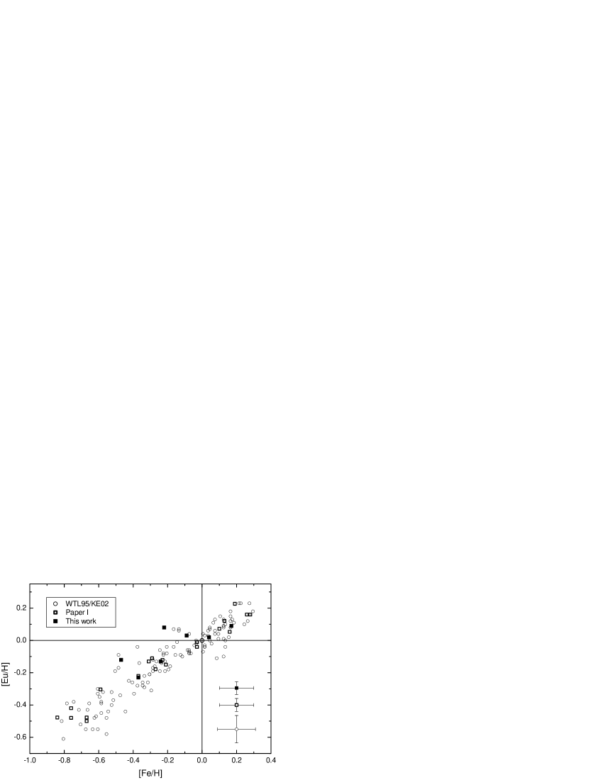
Figure 3: [Eu/H] vs. [Fe/H] diagram for our sample stars, and those from Paper I, WTL95, and KE02. Average error bars for the three data sets are provided in the lower right corner.

Th spectral synthesis employed CES spectra fed by the 3.60 m ESO telescope, whereas the abundances in Paper I were obtained with the CES fed by the CAT. Our results were converted to the CAT system, using the equation derived in Sects. 5.2.1 of Paper I (see their Fig. 20): $\mathrm{[Th/H]}_{\mathrm{CAT+CES}}=-0.01500+0.86000\,\mathrm{[Th/H]}_{\mathrm{CAT+3.60\leavevmode\nobreak\ m}}$.

In Fig. 4, we compare our [Eu/H] abundance ratios to those from Morell et al. (1992, MKB92) and Paper I. These are the best works available with Th abundances for Galactic disk stars, in terms of care of analysis and sample size. Our results are in good accord with them.

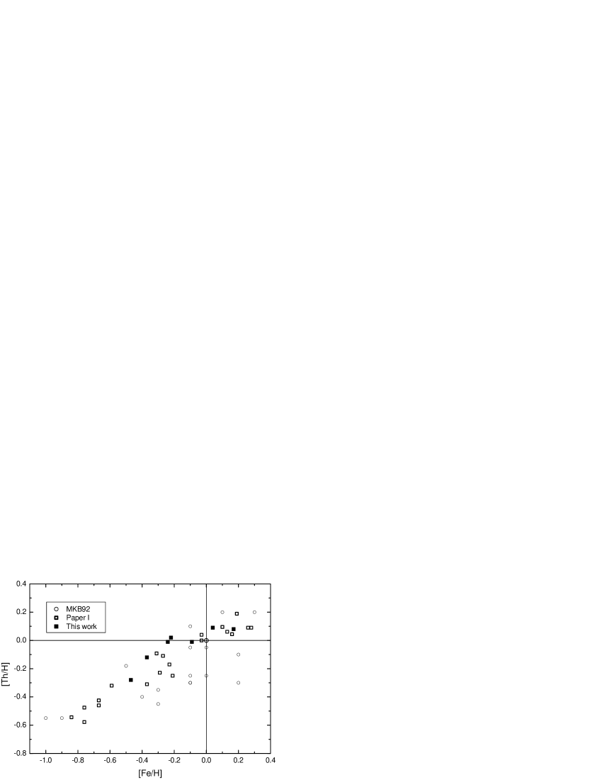
Figure 4: [Th/H] vs. [Fe/H] diagram for our sample stars, and those from Paper I and MKB92. Our results are in good accord with MKB92, but show a lower dispersion.

6 Chronological analysis

In order to estimate the age of the Galactic disk, we compared the stellar [Th/Eu] abundance ratios with curves calculated using a Galactic disk chemical evolution (GDCE) model. In this model, developed by us based on Pagel & Tautvaišienė (1995), it was assumed that the so-called “universality of the r-process abundances” is valid for second and third r-process peaks and can be extended to the actinides. Such extension may not be legitimate, as two ultra-metal-poor stars – CS 31 082-001 (Cayrel et al. 2001 and Hill et al. 2002) and CS 30 306-132 (Honda et al. 2004) – have been recently shown to have Th/Eu abundance ratios much higher than expected for their age. This could indicate that they have been formed from matter enriched in actinides, relatively to second r-process peak elements. However, it is not yet clear if CS 31 082-001 and CS 30 306-132 are merely chemically peculiar objects or if their discrepancies could be present in other yet unobserved stars. A detailed description of the GDCE model was presented in Paper II.

The abundances for our sample were determined in exactly the same way as those from Paper I, as the objective of this work is to expand the sample used for chronological analysis. Accordingly, we merged our abundance data with those from Paper I, resulting in a set of 28 objects. The theoretical model curves and the observed abundance data are presented in Fig. 5.

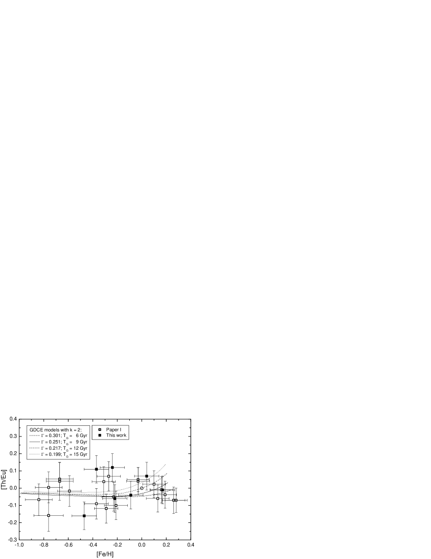
Figure 5: [Th/Eu] vs. [Fe/H] diagram for our sample stars and those from Paper I. Curves were calculated using our GDCE model for the four different Galactic disk ages shown in the legend.

The age of the curve that best fits the observed data was computed by minimizing the total deviation between the curves and the data. 26 of the 28 objects in the merged sample were actually used in the determination; two objects from Paper I were disregarded because they are too metal-rich, falling out of the interval where the curves are defined. Considering that in Paper II 19 objects were actually employed in the analysis, this work accomplishes a 37% increase in sample size. An uncertainty for the age, related solely to the uncertainties in the abundances, was computed through a Monte Carlo simulation. It must be noted that this is only an assessment of the internal uncertainty of the analysis, and does not take into consideration the uncertainties of the GDCE model itself, which are very difficult to estimate. The uncertainty related to the model could very well be the main source of age uncertainty. These procedures are fully described in Paper II. The final value obtained using the merged abundance data set is $(8.8\pm 1.8)\leavevmode\nobreak\ \mathrm{Gyr}$. This result, 0.6 Gyr larger and with an uncertainty 0.1 Gyr lower than that of Paper II, matches very well the estimate obtained from literature data and the GDCE model ($8.7^{+5.8}_{-4.1}\leavevmode\nobreak\ \mathrm{Gyr}$). These estimates were combined using the maximum likelihood method, assuming that each one follows a Gaussian probability distribution, which results in a weighted average using the reciprocal of the square uncertainties as weights. The final, adopted Galactic disk age is

$$T_{\mathrm{G}}=(8.8\pm 1.7)\leavevmode\nobreak\ \mbox{Gyr.}$$

7 Conclusions

We determined [Th/Eu] abundance ratios for a sample of seven Galactic disk F8–G5 dwarfs and subgiants. The analysis was carried out in exactly the same way as that of Paper I, so that we could merge the data, resulting in a totally homogeneous extended sample of 28 objects; 26 of these were actually used in the nucleocosmochronological analysis. A GDCE model, developed in Paper II, was used in conjunction with the stellar abundance data to compute an age for the Galactic disk: $(8.8\pm 1.8)\leavevmode\nobreak\ \mathrm{Gyr}$. In Paper II, Th/Eu production and solar abundance ratio data taken from the literature were analyzed with our GDCE model, yielding $8.7^{+5.8}_{-4.1}\leavevmode\nobreak\ \mathrm{Gyr}$. These two results were combined using the maximum likelihood method, resulting in $\mbox{FINAL }T_{\mathrm{G}}=(8.8\pm 1.7)\leavevmode\nobreak\ \mbox{Gyr}$.

The inclusion of seven more stars in the abundance data base had two main consequences: it increased the age obtained from our stellar data by 0.6 Gyr, rendering it more compatible with the age determined from literature data, and it decreased the uncertainty of the final, adopted age by 0.1 Gyr, i.e., a 6% reduction. Our result remains compatible with the most up-to-date white dwarf ages derived from cooling sequence calculations, which indicate a low age ($\lesssim 10\leavevmode\nobreak\ \mathrm{Gyr}$) for the disk (Oswalt et al. 1995; Bergeron et al. 1997; Leggett et al. 1998; Knox et al. 1999; Hansen et al. 2002). Considering that the age of the oldest halo globular clusters are currently estimated at $(13.5\pm 0.7)\leavevmode\nobreak\ \mathrm{Gyr}$ (Pont et al. 1998; Jimenez 1999; Gratton et al. 2003; Krauss & Chaboyer 2003), an hiatus of $(4.7\pm 1.8)\leavevmode\nobreak\ \mathrm{Gyr}$ between the formation of halo and disk must be taken into consideration in future Galactic formation models.