IRAS 16293$-$2422: proper motions, jet precession, the hot core, and the unambiguous detection of infall

Abstract

We present high spatial resolution observations of the multiple protostellar system IRAS 16293$-$2422 using the Submillimeter Array (SMA) at 300 GHz, and the Very Large Array (VLA) at frequencies from 1.5 to 43 GHz. This source was already known to be a binary system with its main components, A and B, separated by $\sim 5^{\prime\prime}$. The new SMA data now separate source A into two submillimeter continuum components, which we denote Aa and Ab. The strongest of these, Aa, peaks between the centimeter radio sources A1 and A2, but the resolution of the current submillimeter data is insufficient to distinguish whether this is a separate source or the centroid of submillimeter dust emission associated with A1 and A2. Archival VLA data spanning 18 years show proper motion of sources A and B of 17 mas yr^-1, associated with the motion of the $\rho$ Ophiuchi cloud. We also find, however, significant relative motion between the centimeter sources A1 and A2 which excludes the possibility that these two sources are gravitationally bound unless A1 is in a highly eccentric orbit and is observed at periastron, the probability of which is low. A2 remains stationary relative to source B, and we identify it as the protostar which drives the large-scale NE–SW CO outflow. A1 is shock-ionized gas which traces the location of the interaction between a precessing jet and nearby dense gas. This jet probably drives the large-scale E–W outflow, and indeed its motion is consistent with the wide opening angle of this flow. The origin of this jet must be located close to A2, and may be the submillimeter continuum source Aa. Thus source A is now shown to comprise three (proto)stellar components within $1^{\prime\prime}$. Source B, on the other hand, is single, exhibits optically-thick dust emission even at 8 GHz, has a high luminosity, and yet shows no sign of outflow. It is probably very young, and may not even have begun a phase of mass loss yet.

The SMA spectrum of IRAS 16293$-$2422 reports the first astronomical identification of many lines of organic and other molecules at 300 and 310 GHz. The species detected are typical of hot cores, the emission from which is mainly associated with source A. The abundances of second generation species, especially of sulphur-bearing molecules, are significantly higher than predicted by chemical models for this source to date, and we suggest that shocks are probably needed to explain these enhancements. The peaks in the integrated emission from molecules having high rotation temperatures coincide with the centimeter source A1, also highlighting the key role of shocks in explaining the nature of hot cores. Finally, we use the high brightness temperature of the submillimeter dust emission from source B to demonstrate the unambiguous detection of infall by observing redshifted SO ($7_{7}$$-$$6_{6}$) absorption against the emission from its dust disk.

1 Introduction

Our understanding of the formation of binary and multiple stellar systems in clusters lags significantly behind that of isolated star formation, and yet this is the mode in which most stars form. The origin of the problem is the following: the distribution of the companion-star fraction for T Tauri stars and field G dwarfs peaks at separations $\sim 40$–60 AU (e.g., Patience et al. 2002), while the ability to resolve structure on these size scales during the star formation process, when the protostars are deeply embedded and invisible at optical and infrared wavelengths, is not yet routinely available. Distinguishing between the possible binary formation mechanisms, such as prompt fragmentation during collapse or the formation of instabilities in massive disks (Tohline 2002), therefore remains difficult. Until the instruments needed to test these theories observationally become available, we must focus on identifying binary protostars and on understanding their interactions with their immediate environments.

IRAS 16293$-$2422 was one of the first protostars to be identified as a potential binary system, based on the separation of the millimeter continuum emission into two peaks (Mundy, Wilking, & Myers 1986), and on the detection of centimeter radio continuum emission from each component (Wootten 1989). Since then it has been extensively studied using single-dish telescopes and interferometers, and has been found to drive two separate CO outflows (Mizuno et al. 1990; Stark et al. 2004). To date it has been assumed that each of the binary components drives one of the outflows, although the northern binary component, source B, exhibits very narrow linewidths and little evidence of high velocity gas close to the source. This latter fact led Stark et al. (2004) to propose that source B is a T Tauri star and that the outflow it drove in the past is now a fossil flow, but this interpretation also has its problems. Thus it is not even clear yet which sources drive which outflows. IRAS 16293$-$2422 also exhibits strong emission from organic and other species more typically associated with hot cores in massive star-forming regions (e.g., van Dishoeck & Blake 1998), especially at the position of the southern component, source A (Bottinelli et al. 2004; Kuan et al. 2004).

IRAS 16293$-$2422 was also one of the first sources for which the detection of infall in the surrounding envelope was claimed (Walker et al. 1986), based on redshifted self-absorption observed in a line of CS. The presence of the outflows and other velocity gradients across the cloud core made the claim controversial, however (Menten et al. 1987; Narayanan, Walker, & Buckley 1998). There remain, therefore, several outstanding issues relating to the nature of the components of the binary system in IRAS 16293$-$2422: the relative evolutionary states of the two components; the origin of the two outflows; the nature of the hot core emission and its relationship to the two binary components; and the dynamics of the gas associated with the two components including the identification of gravitational collapse.

The high spatial resolution now available with the Submillimeter Array (SMA), and the wide bandwidth enabling many spectral lines to be covered simultaneously, makes this an ideal instrument with which to try to answer some of the outstanding questions relating to IRAS 16293$-$2422. The association of this source with strong, spatially-compact dust emission also raises the prospect of excellent image quality using self-calibration techniques (Pearson & Readhead 1984). The particular frequency settings chosen for the SMA observations presented here were aimed at optimizing the possibility of detecting the high dipole-moment molecule H₂CO in absorption against the compact dust emission, as discussed in Section 4.4.

Many observations of IRAS 16293$-$2422 have also been made using the Very Large Array (VLA) over the years, establishing one of the longest time baselines for high-resolution centimeter radio measurements of any source. Here we combine new SMA data with an analysis of archival VLA data spanning 18 years, shedding new light on the nature of the centimeter and millimeter sources embedded in the cloud core.

IRAS 16293$-$2422 lies in the L1689 dark cloud within the $\rho$ Ophiuchi star-forming region. The distance to $\rho$ Oph has been reported to be 160 pc based on optical and infrared photometry of stars associated with the $\rho$ Oph cloud (Chini 1981), and more recently a distance of 120 pc was obtained from the reddening of optical Hipparcos and Tycho data (Knude & Høg 1998). The high extinction toward $\rho$ Oph limits optical reddening techniques to the outer edges of the cloud. For this reason, and to enable direct comparison with most of the published literature on IRAS 16293$-$2422, we assume a distance of 160 pc. However, derived quantities that depend on distance are given with $D$ explicit, and if the interpretation of any result depends sensitively on $D$ this is discussed.

2 Observations

2.1 Submillimeter wavelength SMA data

The submillimeter observations of IRAS 16293$-$2422 were made using the SMA located on Mauna Kea, Hawaii. Data were obtained on 2004 June 25 and 2004 July 27, in its “extended” and “compact” configurations respectively. The correlator was configured to cover 2 GHz of bandwidth, centered close to the frequency of the H₂CO $4_{13}\rightarrow 3_{12}$ line at 300.836635 GHz, in the lower sideband of the receiver. The intermediate frequency of the SMA is 5 GHz, giving an upper sideband centered 10 GHz higher. Data are obtained from both sidebands. The instrumental phase and amplitude variations were monitored by observing the nearby calibrators NRAO 530 and PKS J1625$-$2527. Absolute flux calibration was obtained from observations of Callisto and the quasar 3C454.3, which was assumed to have a flux density of 4.6 Jy at 300 GHz. The spectral response of the bandpass was obtained from measurements of 3C454.3 and PKS J1924$-$2914. The uncertainty in the absolute flux calibration is estimated to be 10% for the continuum, but is somewhat worse ($\sim 20$%) for individual channels in the spectral line data because of the signal-to-noise ratio obtained for the bandpass calibration.

The 2 GHz total bandpass was divided into 24 overlapping correlator segments. Twenty-three of these were set up to have 128 channels covering 104 MHz (channel separation 0.8125 MHz). The other segment had 512 channels over the same bandwidth, centered on the H₂CO line, to provide a spectral resolution of 0.203 MHz (0.2 km s^-1). The lower sideband in particular contained several strong emission lines, so a continuum dataset was formed from an average of the line-free channels in the lower and upper sidebands. This continuum emission was then subtracted from the spectral line data. Four of the correlator segments at the high(low) frequency end of the lower(upper) sideband exhibited problems, and have been excluded from the data entirely.

The data were reduced using the SMA data reduction package MIR and also using MIRIAD and AIPS. The continuum emission is strong enough for self-calibration techniques to be used to correct for tropospheric phase fluctuations on timescales shorter than the observations of the phase calibrators. The synthesized CLEAN beam using an AIPS robust weighting of 0, intermediate between natural and uniform to optimize both resolution and sensitivity (Briggs 1995), is $1.91^{\prime\prime}\times 0.90^{\prime\prime}$ at P.A. 24^∘, and the rms noise in the resulting continuum image is 19 mJy beam^-1. This noise level is approximately a factor of 10 times the theoretical noise expected for typical system temperatures of 400 K, and is primarily due to the problems of imaging sources comprising considerable extended emission using a sparse array. The rms noise in continuum-subracted, line-free channels is approximately 3 times theoretical. The primary beam of the SMA at the frequency of these observations is approximately 34^′′ FWHM. None of the images presented here has had a primary beam correction applied for display purposes, but all of the quantitative results have been obtained from images that have been corrected for the response of the primary beam.

2.2 Centimeter wavelength VLA data

We have also retrieved all of the available continuum data for IRAS 16293$-$2422 from the VLA archive that have sufficient resolution to separate components A and B ($\theta_{\rm beam}\lesssim 5^{\prime\prime}$). Most of these have previously been reported in the literature, and Table 1 summarizes the datasets and gives references to the descriptions of those data; the details of the observing parameters can be found in these references. For all the data not previously published, the time-dependent amplitude and phases were calibrated using the quasars PKS J1626$-$2951 or PKS J1625$-$2527, and the absolute flux density scale was obtained from measurements of 3C286. The uncertainty in the overall absolute flux density scale used by the VLA is estimated to be 5% from 0.4 to 15 GHz (Baars et al. 1977), and 10% at 22 and 43 GHz. However, there is some evidence of variability in the emission from source A from multi-epoch VLA measurements (see Section 3.1.2 below), so an overall uncertainty of 10% is also assumed for this source at the lower frequencies where only one epoch is available, namely, 1.5 and 5 GHz. All the data were reduced and imaged using AIPS.

While in general our images and flux densities agree to within 2-$\sigma$ of those previously published, there is one exception. The 15 GHz image from Wootten (1989) shows that source A comprises two objects, denoted A1 and A2, with A1 having a peak flux density per beam approximately three times stronger than A2. Our image, on the other hand, shows that the two components have comparable peak flux densities per beam. The difference arises because self-calibration using the 5 GHz image as a model was applied to the data presented by Wootten. Self-calibration can only improve an image if there is a sufficiently high signal-to-noise ratio in the visibility data; unfortunately, this is not the case for the 15 GHz data, and under these circumstances false source structure can be introduced if self-calibration is used. Our image has not had any self-calibration applied, and we believe it to be more reliable than that presented by Wootten.

All the archival VLA data were observed in B1950 coordinates. For comparison with the SMA data all the VLA data have been precessed to J2000. Furthermore, the position used for one of the phase calibrators, PKS J1626$-$2951, has been refined and improved over the years. All the VLA data using PKS J1626$-$2951 as a phase calibrator have therefore been adjusted to match the latest position in the VLA Calibrator Manual, of R.A. (J2000) = $16^{\rm h}26^{\rm m}06\fs 0208$, dec. (J2000) = $-29^{\circ}51^{\prime}26\farcs 971$. The absolute positions for all the VLA phase calibrators used are good to $\sim 2$ mas.

3 Results

3.1 Continuum emission

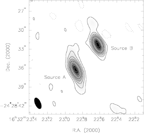
Figure 1: Continuum image of IRAS 16293$-$2422 at $\nu=305$ GHz with CLEAN beam $1.91^{\prime\prime}\times 0.90^{\prime\prime}$ at P.A. $24^{\circ}$, shown at bottom left. Contours are spaced at $-$3, 3, 8, 15, 24, 35, 48, 63, 80, 99, and 120 times the rms noise of 19 mJy beam^-1. The peak 1 mm flux densities for sources A and B are $2.08\pm 0.02$ and $2.63\pm 0.02$ Jy beam^-1 respectively.

The $\lambda=1$ mm SMA continuum image of IRAS 16293$-$2422 is shown in Fig. 1. Integrated flux densities from the SMA and archival VLA data are summarized in Table 2, and plotted in Fig. 2. Where multiple epochs at a particular frequency are available, the error quoted is the standard deviation of the multi-epoch measurements combined with the absolute uncertainty in quadrature. Fig. 2 also includes data points from other measurements reported in the literature that have sufficient resolution to separate sources A and B, at 110 and 230 GHz (Bottinelli et al. 2004) and at 354 GHz (Kuan et al. 2004). Power-law fits to the interferometric data, $F_{\nu}\propto\nu^{\alpha}$, are also plotted for $\nu<100$ GHz and $\nu>100$ GHz. The fact that sources A and B are embedded in extended emission from the surrounding envelope in fact makes the spectral indices derived from formal fits to the $\nu>100$ GHz data rather more uncertain than the errors given in Fig. 2, since no attempt has been made here to match the $u$-$v$ coverage at each frequency. Indeed, that this is a potential problem can clearly be seen for the 230 GHz flux density from Bottinelli et al. (2004), for which the shortest baseline is a factor of $\sim 2$ longer than that of the 110 GHz data. This is also illustrated in the 110 GHz images reported by Looney, Mundy, & Welch (2000). The 230 GHz data have therefore not been included in the fit. Interpolating between the 1.3 mm and 850 $\mu$m total integrated single-dish flux densities from Schöier et al. (2002) using a power law we expect a total 1 mm flux density of 18 Jy; the SMA is therefore filtering out approximately 60% of the continuum emission associated with the extended envelope. At 43 GHz the largest angular scale to which the VLA is sensitive in the A-configuration is 1.3^′′. The 43 GHz measurements available to date seem to be sensitive only to the compact emission components also responsible for the emission at lower frequencies, and are missing flux associated with the more extended emission detected at higher frequencies.

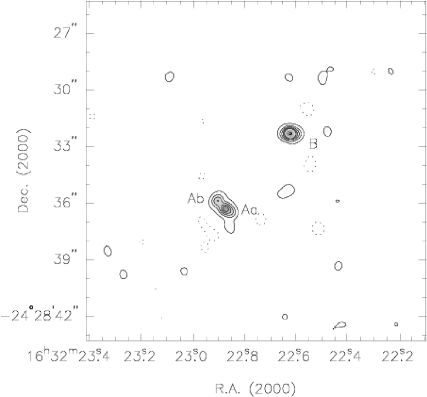
Figure 3: Left: plot of visibility amplitude against $u$-$v$ distance projected along a position angle of $-45^{\circ}$. Right: Continuum image obtained using only data $>55$ k$\lambda$, super-uniform weighting, and a circular restoring CLEAN beam of $0.4^{\prime\prime}$ FWHM. Contours are at the same levels as in Fig. 1.

The 1 mm continuum emission detected by the SMA from sources A and B comprises both extended components and more compact emission. In order to assess the relative contributions from both, we have made an image using only the long baseline data (a lower limit of 55 k$\lambda$ was chosen from inspecting plots of visibility flux versus $u$-$v$ distance, the point at which the circumbinary envelope starts to contribute significantly to the overall flux: see Fig. 3), increasing the relative weights of the longest baselines (super-uniform weighting), and restoring the image with a CLEAN beam of $0.4^{\prime\prime}$, slightly smaller than half the fringe spacing on the longest baseline, $0.54^{\prime\prime}$ (Fig. 3). This image essentially illustrates the location of the CLEAN components derived from the deconvolution of the point spread function, as obtained from the longest baselines present in the data. It is apparent in this “super-resolution” image that while the compact emission from source B remains singly-peaked, source A comprises a compact source close to the position of the overall continuum peak in Fig. 1, along with a second, new source offset by 0.64^′′ to the northeast. This object does not coincide with any of the previously-identified sources in this region (the closest is the centimeter radio source A1, which is $\sim 0.4^{\prime\prime}$ to the southwest), and contains approximately 30% of the flux associated with the compact emission from source A in Fig. 3. We interpret this new source as a candidate protostar. In what follows we denote the stronger of the two components Aa, and the new candidate companion Ab. Table 3 gives positions and flux densities for the compact emission components shown in Fig. 3. The fraction of the flux detected by the interferometer associated with the compact emission shown in Fig. 3 for source A is $\sim 60$%, and for source B is $\sim 90$%.

Since source A is now shown to comprise multiple submillimeter and centimeter radio components we use “source A” to refer to the combination of all components, Aa+Ab+A1+A2. Discussion of an individual component will refer directly to the name of that component.

3.1.1 Proper motion and the relationship between the centimeter and submillimeter sources

In order to investigate the relationship between the submillimeter emission and the radio continuum sources, we first need to account for the proper motion of the sources. The proper motion of sources A and B has been reported previously by Loinard (2002), based on two epochs of VLA 8 GHz data (1989 and 1994), and indicate motion presumably associated with the L1689N cloud in which sources A and B are embedded (see also Curiel et al. 2003). When observed at high resolution the centimeter radio emission from source A comprises two components, denoted A1 (to the east) and A2 (to the west) by Wootten (1989), separated by 0.35^′′. We show below that the overall structure of the centimeter radio emission from source A has been changing with time, so the simpler structure of source B makes measurement of its proper motion more straightforward. In Fig. 4 we plot the position of source B derived from the SMA data, and all the VLA data having a resolution of 1^′′ or better, as a function of time, along with the offset between sources A2 and B, and between A1 and A2, for those measurements which resolve the two components of source A. Fig. 4 demonstrates that the proper motion of sources A2 and B are in common, and that their motion is primarily in declination. The overall proper motion of sources A2 and B, 17 mas yr^-1, corresponds to $13(D/{\rm 160~{}pc})$ km s^-1. Fig. 4 also illustrates significant motion of A1 relative to A2, amounting to $10(D/{\rm 160~{}pc})$ km s^-1.

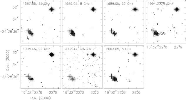
Figure 5: VLA data (contours) overlaid on the 1 mm super-resolution image, after aligning source B in the different epochs. The crosses indicate the positions given in Table 3. The size of the crosses are not proportional to the positional accuracy of the submillimeter sources.

We have corrected for the proper motions described above, and other uncertainties in the absolute positions caused by using different quasars for the phase calibration for some of the measurements, by shifting all the archival VLA to align source B with the 1 mm position in Table 3. Fig. 5 presents the result of overlaying the shifted radio continuum emission on the 1 mm super-resolution continuum image. When observed with sufficient resolution to separate the two centimeter radio sources A1 and A2 it is clear first that their orientation has been changing over the years as indicated in Fig. 4, and second that they lie on either side of the submillimeter continuum source Aa. In Fig. 6 we plot the projected separation between A1 and A2, and their position angle, as a function of time. Considering only the 8 GHz data we might conclude that the separation between A1 and A2 has been increasing slightly, and that the rate at which the position angle is changing is slowing down. However, this conclusion becomes marginal when the results at other frequencies are included. Fig. 4 shows that a linear fit to the position offsets in R.A. and dec. matches the data well. The projected separation between A1 and A2 has remained constant, at $0.35^{\prime\prime}\pm 0.02^{\prime\prime}$, while the position angle is equally well-fitted by a straight line as by a second order polynomial function. The quadratic function shown in Fig. 6 (dotted line) turns over in 2014, so regular monitoring will be needed over the next few years to establish whether the rate of change in position angle is indeed slowing down, as suggested by the three 8 GHz points.

Since the 1 mm SMA data are not able to resolve the separation of the two centimeter radio sources, it is important to establish whether the apparent location of Aa between A1 and A2 in the super-resolution image is real, or whether the location of the CLEAN components just corresponds to the centroid of submillimeter emission associated directly with A1 and A2. To test this we have made simulated images comprising a source at Ab, and sources at the positions of A1 and A2 from epoch 2003.65 (the most recent VLA data) with a total flux that of Aa given in Table 3. We find that for a flux ratio $F_{\rm A2}/F_{\rm A1}$ of unity the peak is indeed located at the observed position of Aa in Fig. 3. For a flux ratio of 1.8, the same as that observed at 8 GHz for this epoch, the peak position would be offset by 0.12^′′, which is more than 6-$\sigma$ away from that measured. We therefore conclude that if the centimeter radio sources A1 and A2 are each associated with dust continuum emission, their submillimeter flux ratio is close to unity. The resulting implications for the nature of Aa, A1, and A2 is discussed further in Section 4.

3.1.2 Source variability

Along with the clear secular structural evolution of the radio emission from source A shown in Fig. 5, there is also evidence for flux variability. Fig. 7 illustrates the integrated flux density for sources A and B as a function of time at 8, 15, and 22 GHz, where the error bars include the absolute flux uncertainty described in Section 2.2. At all three frequencies, source B is consistent with being nonvariable, apart from the earliest 15 GHz measurement which comes from the data first presented by Wootten (1989). These data suffered significantly from poor tropospheric phase stability, and an analysis of images of the phase calibrator for this epoch suggests that the observed flux densities for IRAS 16293$-$2422 are $\sim 20$% too low due to the decorrelation. We have not, therefore, included the flux density measurements from this epoch in the average 15 GHz flux densities plotted in Fig. 2 for sources A and B, and exclude it from our discussion of variability here. Thus we conclude that the flux density of source B is constant in time, at all three frequencies measured.

Source A, on the other hand, clearly exhibits a trend of decreasing flux density between 1988 and 2003 at both 8 and 15 GHz, while the spectral index remains approximately constant. The observations able to separate the centimeter radio components show that the emission from both A1 and A2 has been decreasing, but that A1 is fading faster than A2, with $F_{\rm A2}/F_{\rm A1}\sim 0.7$ around epoch 1990, compared to $\sim 1.8$ in 2003. During this time the position angle of the vector joining A1 and A2 has traversed the position angle of the vector joining the submillimeter components Aa and Ab (see Fig. 5). It is possible that the dramatic variability of A1 has been produced by the interaction of a wind or jet with Ab and/or dense gas in its immediate environment, or from intrinsic variability of the source of ionized gas. The origin and properties of this plasma is discussed further in Section 4.1.

Possible short term variability of the 15 GHz radio emission has been investigated by Estallela et al. (1991) between 1987 and 1988. No evidence for variability on timescales of several hours to a year was found by those authors, but this is consistent with the variability of source A on longer timescales, as demonstrated by Fig. 7.

3.2 Spectroscopy

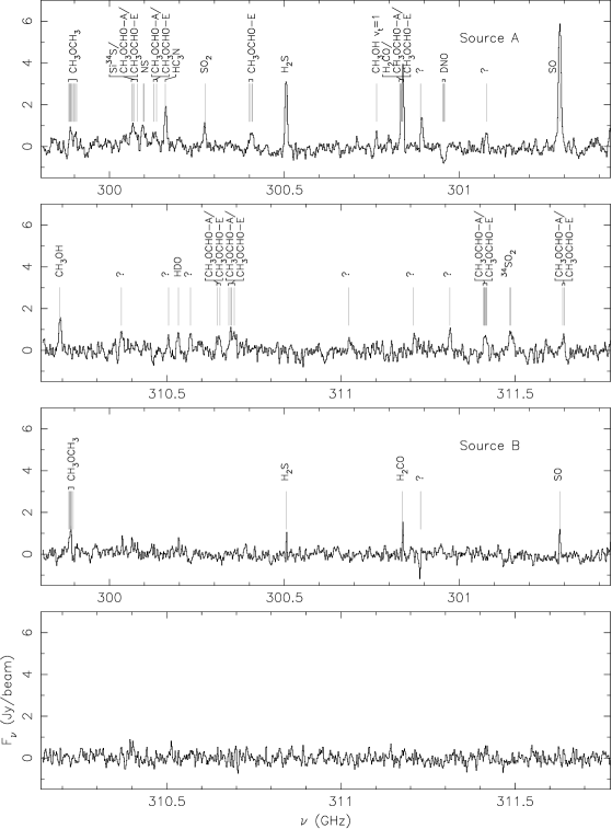
Figure 8: Spectra of the lower and upper sidebands in the SMA data smoothed over 4 channels (3.25 MHz) for source A (top two panels) and source B (bottom two panels).

All the molecular line emission was imaged with an AIPS robust weighting parameter of 2, close to natural weighting, to give the best sensitivity. The resulting synthesized CLEAN beam is $2.45^{\prime\prime}\times 1.22^{\prime\prime}$ at P.A. $31^{\circ}$ for both lower and upper sidebands. Fig. 8 shows the full lower and upper sideband spectra for sources A and B, averaged over boxes approximately $1.5^{\prime\prime}\times 1.5^{\prime\prime}$ in size. Only one other spectrum covering $\nu\sim 300$ GHz has been reported in the literature, a low spectral resolution (200 MHz) observation of the Orion molecular cloud core by Serabyn & Weisstein (1995). Fig. 8 therefore shows the first astronomical detection of many of the lines indicated. Line identifications have been obtained from a comparison with the spectral line catalogs of Pickett et al. (1998) and Müller et al. (2001). Line identifications are particularly difficult for the weak transitions of organic species, for which many potential blends are possible within a typical linewidth of a few MHz. Firm identifications of organic molecules have therefore only been made when all transitions lying within the lower or upper sideband are observed with the expected relative line strengths. The main organic species that have been detected are dimethyl ether (CH₃OCH₃), A- and E-type methyl formate (CH₃OCHO), cyanoacetylene (HC₃N), methanol (CH₃OH), and formaldehyde (H₂CO). A possible line of Si³⁴S may be blended with methyl formate emission. Other significant species detected are the sulphur-bearing molecules NS, SO₂, H₂S, and SO, and the deuterated species DNO (in absorption) and HDO. Several lines remain unidentified, emphasizing the need for more complete line lists for complicated organic molecules at submillimeter wavelengths. Table 4 summarizes the transitions of all molecules observed, and gives integrated line fluxes for positively-identified lines not blended with emission from other species, and also for H₂CO, which is blended with methyl formate emission.

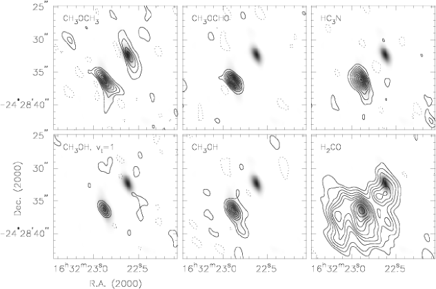
Figure 9: Location of emission from organic species detected towards IRAS 16293$-$2422. The emission from CH₃OCH₃ is the sum of both the 5$-$4 and 8$-$7 transitions in Table 4, and the CH₃OCHO image is made from the sum of all A- and E-type lines not blended with other species. For all images apart from H₂CO the contours are linearly spaced at approximately 2$\sigma$ intervals of 2.43 (CH₃OCH₃), 1.97 (CH₃OCHO), 1.96 (HC₃N), 1.53 (CH₃OH, $v_{t}=1$), and 2.34 (CH₃OH) Jy km s^-1. For H₂CO the contours are at $-$1, 1, 2, 3.5, 5, 6.5, 8, 10, 12, 14, 17, and 20 times 2.04 Jy km s^-1.

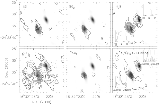
Figure 10: Emission from sulphur-bearing species. For display purposes the H₂S emission is integrated over the width of the narrow line associated with source B, to avoid spectral dilution. Spectra of sources A and B are also plotted in the bottom left corner (source A) and top right corner (source B) of the H₂S panel. In the bottom right panel the emission is integrated over the line marked in Fig. 8 as Si³⁴S/CH₃OCHO-A/CH₃OCHO-E. Unsmoothed spectra are also plotted for source A (bottom left corner) and source B (top right corner) in this panel, with the locations of the lines indicated: the Si³⁴S line is marked explicitly, and the other three lines are transitions of methyl formate, as listed in Table 4. For all images apart from SO the contours are linearly spaced at approximately 2$\sigma$ intervals of 1.43 (NS), 2.00 (SO₂), 1.02 (H₂S), 1.98 (³⁴SO₂), and 2.59 (Si³⁴S) Jy km s^-1. For SO the contours are at $-$1, 1, 2, 3.5, 5, 7, 9, 12, 15, 19, 23 and 28 times 2.62 Jy km s^-1.

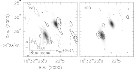
Figure 11: Emission and absorption from deuterated species. Contours are linearly spaced at approximately 2$\sigma$ intervals of 2.80 (DNO), and 2.64 (HDO) Jy km s^-1. Dotted contours are negative. DNO is detected in absorption toward source A, and its unsmoothed spectrum, with the location of DNO lines indicated, is in the bottom left of the DNO panel.

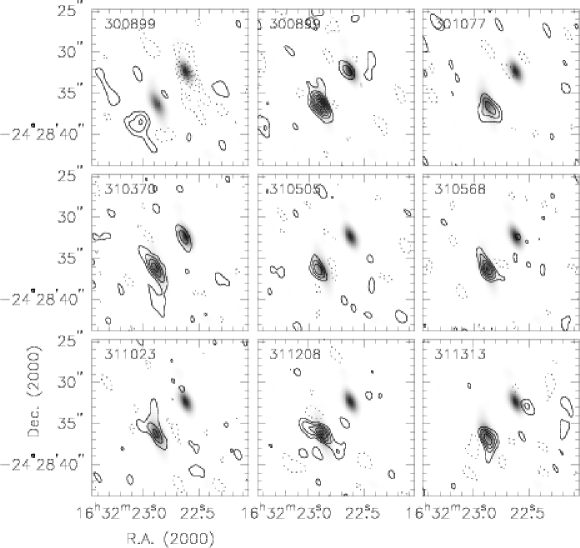
Figure 12: Emission from unidentified lines. Each panel is marked with the approximate center rest frequency of the line in MHz. In the case of the 300899 MHz line, there is a feature detected in absorption toward source B to the redshifted side of the strong emission line observed toward source A. It is possible that these originate from completely different lines, but in the absence of further information they have both been designated as 300899 MHz here. All contours are linearly spaced at approximately 2$\sigma$ intervals.

Lines detected at 6$\sigma$ or better in integrated emission (corresponding approximately to a flux density cutoff of 0.7 Jy beam^-1 in Fig. 8) are displayed in Figs. 9–12, showing that the molecular line emission is centered close to source A, with some species also exhibiting emission coincident with source B. Unlike the results for H₂CCO and $c$-C₃H₂ reported by Kuan et al. (2004), none of the molecules we detect in emission are associated only with source B and not source A. There is, however, a significant detection of absorption toward source B in an unidentified line.

Single-dish observations have indicated the presence of three separate physical and chemical components in IRAS 16293$-$2422: a cold, outer envelope with $T\sim 10$–20 K, a circumbinary envelope with $T\sim 40$ K approximately $10^{\prime\prime}$ in size, and a compact, warm component ($T\gtrsim 80$ K) only a few arcsec in extent (van Dishoeck et al. 1995; Ceccarelli et al. 2000). Of course, there is probably a continuous temperature gradient throughout the envelope, with these size scales representing temperatures at which molecules are liberated from the surface of dust grains, and where ice mantles evaporate (Schöier et al. 2002; Doty, Schöier, & van Dishoeck 2004). Subsequent gas-phase chemistry can then cause significant jumps in the abundances of certain species. Further, gas phase abundances, particularly of sulphur-bearing species, can be dramatically changed by the passage of a shock (Wakelam et al. 2004a; Viti et al. 2001).

The presence of these different regimes in the envelope mean that single-dish measurements of beam-averaged column densities, and their conversion to abundances through comparison with (single-dish) beam-averaged H₂ column densities, will not give good estimates of the local abundance. To minimize this problem for our interferometer data we do the following. Molecular column densities have been calculated by integrating over emission regions having a signal-to-noise ratio $\geq 2\sigma$, using rotation temperatures derived from rotation diagrams (cf. Goldsmith & Langer 1999) either reported previously in the literature, or from new analyses presented below. The corresponding molecular hydrogen column densities for determining local abundances are obtained from a 1 mm SMA dust continuum image made with the same weighting and beam size as the molecular line data, and masked to match the extent of the molecular emission. We adopt a 300 GHz dust opacity $\kappa_{\rm 300~{}GHz}=1.5$ cm² g^-1, a gas to dust ratio $M_{\rm g}/M_{\rm d}=100$, and $T_{\rm dust}=40$ K, as described in Section 4.1.

The H₂ column density derived from the dust emission is inversely proportional to the assumed temperature, but since the line of sight towards sources A and B probably includes emission from dust at $\sim 20$ to 80 K, a value of 40 K will not introduce errors of more than a factor of 2 or 3. Other sources of uncertainty are likely to dominate the derived abundances, such as the uncertainty in the absolute value of the dust opacity, the uncertainty in the assumed rotation temperatures, the presence of temperature gradients in the emission regions, and the assumption of local thermodynamic equilibrium. Table 5 summarizes the derived or assumed rotation temperatures, and the average column densities and abundances for each molecule. The abundances for sources A and B cannot be separated due to the dependence of the rotation temperature estimates on single dish data: even the new estimates presented below use supplemental single dish data from the literature. Thus, only a composite abundance is listed in Table 5. Instances where there is circumstantial evidence of a significant difference between the two sources are noted below in comments on the individual molecular species.

In the notes below we also compare the derived abundances with previous attempts to model or predict chemical abundances in IRAS 16293$-$2422 by Schöier et al. (2002) and Doty et al. (2004); the model abundances from these studies are also presented in Table 5. The Schöier et al. (2002) model is based on a detailed analysis of the radiative transfer of the observed single dish continuum and molecular line emission from IRAS 16293$-$2422. This model uses the derived density and temperature profiles as a function of radius from analysis of the continuum data to determine empirically the best fit to the molecular line data by varying the abundances as a function of radius. In contrast Doty et al. (2004) use the density profile derived by Schöier et al. (2002) and the UMIST chemical network database (Millar, Farquhar, & Willacy 1997) to determine directly the temperature profile and the abundances as a function of time and radius. In order to compare these models with our SMA data we only consider the abundances reported by Schöier et al. and Doty et al. on small size scales, corresponding to $r<2.5\times 10^{15}$ cm (i.e., $1\arcsec$ at 160 pc). Further comparison of these model results and our data are presented in Section 3.2.5.

3.2.1 Organic species

The compact, warm component of the envelope shows many features in common with the hot cores usually associated with more massive star-forming regions, albeit on a much smaller size scale. In such hot cores, the hydrogenated “first-generation” molecular species released from ices on the dust grains, such as H₂CO and CH₃OH, then form the basis of further gas-phase chemical reactions to form more complex “second-generation” species, such as CH₃OCH₃ and CH₃OCHO (e.g., Charnley, Tielens, & Millar 1992). Initial attempts to detect these second-generation, complex organic molecules toward IRAS 16293$-$2422 using single-dish telescopes provided only upper limits (van Dishoeck et al. 1995), and Schöier et al. (2002) interpreted this to mean that the time needed to form these molecules is not available on such small scales in an infalling envelope close to a low-mass protostar. However, very compact emission from several complex organic species has now been reported by Bottinelli et al. (2004) and Kuan et al. (2004), and is also shown in Fig. 9, suggesting that the earlier non-detections were due to beam dilution. A range of emission structure is exhibited by the organic molecules detected in our SMA study (see Fig. 9), from the unresolved emission from a high-energy transition of torsionally-excited methanol, to extended emission from formaldehyde.

CH₃OCH₃

Dimethyl ether is associated with both sources A and B. Cazaux et al. (2003) have also detected emission from 7$-$7, 8$-$7, and 14$-$13 transitions using the IRAM 30m telescope, and we plot a rotation diagram including these data in Fig. 13, from which the rotation temperature and total column density listed in Table 5 is derived. Chemical models require high gas-phase abundances of methanol to produce dimethyl ether (Millar, Herbst, & Charnley 1991), and timescales $\sim 10^{4}$–$10^{5}$ yr. The abundance measured here, $\sim 8\times 10^{-8}$, is similar to that predicted by models for the Orion compact ridge, where the grain mantles are rich in methanol (Charnley et al. 1992; Caselli, Hasegawa, & Herbst 1993). However, it is significantly in excess of that predicted by the physical-chemical modeling of IRAS 16293$-$2422 by Doty et al. (2004), who obtain a maximum value of $\sim 3\times 10^{-9}$. The Schöier et al. (2002) model predicts a dimethyl ether abundance of $<4\times 10^{-8}$, within a factor of two of the SMA value.

CH₃OCHO

The large number of transitions detected from A- and E-type methyl formate are unfortunately severely blended throughout the spectrum, and we have made no attempt to separate them to provide independent column density and abundance measurements. The image shown in Fig. 9 comprises all the emission from both A- and E-type methyl formate not blended with other species. Note that unlike the methyl formate images presented by Bottinelli et al. (2004) and Kuan et al. (2004), we do not detect any methyl formate emission associated with source B. In the case of the Bottinelli et al. result this may be explained by the fact that these authors observed somewhat lower energy transitions than those presented here, consistent with the gas excitation temperatures (and CH₃OCHO column density) at source B being lower than for source A. However, the methyl formate transitions detected by Kuan et al. toward source B are higher in energy, which is difficult to reconcile with the upper limit of our non-detection (about a factor of two less than their detection). The formation of methyl formate is thought to arise from chemical reactions involving either formaldehyde or methanol when these species are evaporated from the surface of dust grains (e.g., Horn et al. 2004) both of which are primarily associated with source A (Fig. 9).

HC₃N

The emission from the relatively high energy level transition of HC₃N is compact and associated with source A, and the rotation diagram for this molecule (Fig. 13) also indicates high temperatures on these size scales (Table 5). However, there is clearly also emission from the more extended, cooler, envelope, and the $J$=5$-$4 flux reported by Suzuki et al. (1992) lies considerably above the best-fit $T_{\rm rot}\sim 320$ K obtained using only the higher-lying transitions. The abundance derived, $1\times 10^{-9}$, is in good agreement with those obtained for the inner envelope from an analysis of single-dish data (Schöier et al. 2002), but is an order of magnitude higher than that predicted by Doty et al. (2004) for small size scales, of $\sim 1\times 10^{-10}$.

CH₃OH

Methanol is detected in both its ground and first torsionally-excited states. The ground state emission is fairly compact with a slight NE-SW extension. The emission from the $v_{t}=1$ line is unresolved, but offset by +0.1^′′ in R.A. from the continuum position of Aa, close to A1. This line has the highest energy of any of the transitions observed, with $E_{\rm upper}=732.4$ K. Since only one transition of the torsionally-excited state was observed we regard this detection as tentative until other lines have been identified.

The rotation temperature derived from many lines of CH₃OH by van Dishoeck et al. (1995) has been used in calculating the column density and abundance from the ground and torsionally-excited state emission in Table 5. Both the column densities and abundances are in good agreement with the models of Schöier et al. (2002) and Doty et al. (2004).

H₂CO

The formaldehyde emission is very extended and originates from both the warm, compact, inner envelope, and the $\sim 40$ K circumbinary envelope. The peak line brightness temperature is 42 K, indicating that especially toward source A the emission has significant optical depth. The H₂CO emission is unfortunately blended with several lines of methyl formate that fall on the low frequency side of the formaldehyde line. Using the column densities derived by Cazaux et al. (2003) for methyl formate (and noting that these authors assumed a size of 2^′′ for the emitting region), rotation temperatures between 65 and 100 K give potential contributions to the integrated flux in the formaldehyde line reported in Table 4 of 5–10%. We have subtracted 5% (corresponding to $T_{\rm rot}\sim 65$ K) from the integrated flux, and use the rotation temperature derived by van Dishoeck et al. (1995) of 80 K for deriving H₂CO column densities and abundances in Table 5. An abundance of $\sim 1\times 10^{-7}$ matches those predicted on small size scales by the Schöier et al. and Doty et al. models to within a factor of 2. The column density also matches the models reasonably well, when it is taken into account that there is considerable extended formaldehyde emission from the envelope that has been resolved out by the interferometer (see also Schöier et al. 2004).

3.2.2 Sulphur-bearing species

NS

Our detection of NS is the first reported for IRAS 16293$-$2422. In deriving its column density and abundance we have assumed a temperature of 100 K, similar to that observed for the other hot core species. Viti et al. (2001) predict that the abundance of NS is significantly enhanced by shocks, and that a high NS/CS abundance ratio is indicative of the evaporation of grain mantles with subsequent chemical processing over a few $\times 10^{4}$ yr. Comparison with the CS abundance derived by Blake et al. (1994) gives NS/CS $\sim 0.6$ for IRAS 16293$-$2422, similar to the Viti et al. models that require the grain mantles to have evaporated early on, enabling significant subsequent chemical processing. However, whether the evaporation is caused by sputtering in shocks or by thermal evaporation is less easily determined from the models using just the NS/CS ratio.

H₂S

H₂S emission is associated with both sources A and B, with the emission at B having a much narrower line width, as has been observed in some other species (e.g., Kuan et al. 2004; also see the H₂S profile insets in Fig. 10). Its emission is somewhat extended, and the rotation diagram gives $T_{\rm rot}=60$ K (Fig. 14). However, the observed abundance, $\sim 9\times 10^{-8}$, is significantly higher than that predicted by the Doty et al. model, for which $\sim 3\times 10^{-9}$ is obtained at $t=3\times 10^{3}$ yr, and $\lesssim 10^{-11}$ for $t=3\times 10^{4}$ yr. However, our abundance estimate for H₂S is in very good agreement with that predicted by Schöier et al. (2002). The narrower line width of H₂S toward source B suggests that the column density and abundance toward this source may be lower than the composite value given in Table 5.

SO and SO₂

SO and SO₂ are formed in the gas phase, but may also be present in grain mantles. The SO₂ emission reported here originates from the highest energy SO₂ transition reported so far in the literature for IRAS 16293$-$2422 ($E_{\rm upper}=519.1$ K). The emission lies significantly above the best fit to the rotation diagram presented by Blake et al. (1994) of $T_{\rm rot}=95$ K, and results in considerable curvature in that rotation diagram indicative of the presence of temperature gradients. Using only those lines with $E_{\rm upper}>200$ K, we find $T_{\rm rot}\sim 135$ K for the compact emission (Fig. 14), and have used this in deriving the column density and abundances for both SO₂ and ³⁴SO₂. The resulting isotopic ratio is $N$(SO₂)/$N$(³⁴SO₂) = 17, similar to that derived for S/³⁴S from CS in the interstellar medium, of $\sim 22$ (Wilson & Rood 1994). The measured abundance for SO₂, $\sim 1\times 10^{-7}$, is an order of magnitude higher than that predicted by Doty et al. (2004) of $1\times 10^{-8}$, but is in good agreement with the analysis of Schöier et al. (2002).

The SO line is the strongest in the entire spectrum. Its peak line brightness temperature is 46 K, indicating significant optical depth. Indeed, Blake et al. (1994) derive their rotation temperature of 80 K from the ³⁴SO isotopomer instead, because of high optical depth in the transitions of SO they observed. The measured abundance, $5\times 10^{-7}$, is two orders of magnitude higher than that predicted by Doty et al. (2004), of $\sim 4\times 10^{-9}$. The SO abundance in the Schöier et al. (2002) model is within a factor of two of our estimate.

Si³⁴S

We also report the possible detection of Si³⁴S, although it is blended with both A- and E-type methyl formate emission, and should at present be regarded as tentative.

3.2.3 Deuterated species

The envelope surrounding IRAS 16293$-$2422 exhibits remarkably high abundances of deuterated species. Bright, extended D₂CO has been observed (Ceccarelli et al. 1998, 2001; Loinard et al. 2000), and even triply-deuterated methanol, CD₃OH (Parise et al. 2004a). Typical fractionations are 5–20%, depending on the species (e.g., Roberts et al. 2002; Parise et al. 2004a). High deuterium fractionation is thought to be the result of grain surface chemistry under low temperature conditions, and the deuterated molecules are observed when they are subsequently desorbed back into the gas phase (Ceccarelli et al. 2001).

DNO

Here we report the probable detection of deuterated HNO in absorption against source A. DNO has the best match in frequency for the absorption feature at 300955 MHz, but there are no other reports of either HNO or DNO observations in the literature for IRAS 16293$-$2422. For other sources, however, Snyder et al. (1993) and Ziurys, Hollis, & Snyder (1994) suggest a NO/HNO abundance ratio of $\sim 100$–800, and van Dishoeck et al. (1995) report an upper limit for a NO line towards IRAS 16293$-$2422. Unfortunately this upper limit is for a high energy transition, and so does not give a very stringent upper limit on the NO column density, $N$(NO) $<1\times 10^{19}$ cm^-2 (2$\sigma$). Both NO and HNO are expected to be associated with the cooler, outer envelope in IRAS 16293$-$2422 (see the predicted column densities of Doty et al. 2004), and the energy of the 300955 MHz transitions are relatively low, consistent with observing this line in absorption and resolving out much of the extended emission from the envelope. The optical depth of the absorption feature is $\approx 0.45$, which for an excitation temperature of 15–20 K implies a column density $N$(DNO) $\sim 3\times 10^{15}$ cm^-2. This is consistent with the NO upper limit if NO/HNO $\sim 300$, and DNO/HNO $\sim 0.1$.

HDO

We also detect a relatively high-energy transition of deuterated water, HDO. Parise et al. (2004b) have recently performed an analysis of the HDO abundance in different components of the envelope of IRAS 16293$-$2422, finding a considerably higher abundance in the inner region, where the ices have evaporated from the dust grains, compared with the outer envelope. Fig. 11 shows that the emission region for the high-energy transition is indeed very compact. In Fig. 15 we show the rotation diagram for HDO, including other data from the literature. The one point that lies significantly away from the best-fit line for $T_{\rm rot}=236$ K is a measurement from Parise et al. (2004b) obtained with a 10^′′ beam pointed at source B. Since the HDO emission is in fact associated with source A, the emission was probably close to the half-power point of the beam (or worse, if the pointing was off by only a few arcsec). We have therefore not used this point in the fit. The derived abundance is about a factor of 4 lower than that obtained by Parise et al.

3.2.4 Unidentified lines

Emission from a number of unidentified lines is detected, primarily associated with source A (Fig. 11). The 300899 MHz line is particularly bright, and has immediately to its redshifted side a strong absorption toward source A. It is possible that these originate from completely different lines, but in the absence of further information they have both been designated as 300899 MHz here.

3.2.5 Comparison with the physical-chemical model for IRAS 16293$-$2422

In general the physical-chemical model of Doty et al. (2004) on small size scales matches well the observed abundances of first generation precursors of organic species, i.e., H₂CO and CH₃OH, but the abundance of second generation molecules, CH₃OCH₃ and HC₃N, are underestimated by about an order of magnitude. For the sulphur-bearing species all abundances are underestimated by the physical-chemical model of Doty et al. (2004) by one to two orders of magnitude. Overall the agreement with the empirical model of Schöier et al. (2002) on small size scales is much better. These results suggest that the chemistry of first generation species is well understood, but that of second generation organic molecules and sulphur bearing species are not (see also the discussion of Doty et al. 2004).

There are two possible explanations for the low abundances of sulphur bearing species in the Doty et al. (2004) model. First, Wakelam et al. (2004a) have recently shown that the abundances of sulphur-bearing species such as SO, SO₂, and H₂S in the hot core phase are strongly dependent on the assumed form and abundance of sulphur-bearing species on the dust grains before evaporation. Moreover, a number of recent experiments suggest that H₂S cannot be the sole carrier of sulphur on dust grains (see, e.g., Wakelam et al. 2004a; van der Tak et al. 2003, and references therein). Indeed, Wakelam et al. (2004a) find the best agreement with observations of both Orion and IRAS 16293$-$2422 for the following ice composition: H₂S, $10^{-7}$; OCS, $10^{-7}$; and S, $3\times 10^{-6}$ (atomic sulphur in molecular matrix). In contrast, Doty et al. (2004) assume that initially all of the sulphur is in the form of H₂S. Doty et al. (2002) report results from using a chemical network analysis for the high mass hot core AFGL 2591 similar to that used for their more recent study of IRAS 16293$-$2422. In order to obtain a good fit to the observed AFGL 2591 hot core SO₂ abundance, Doty et al. (2002) adjusted the initial H₂S abundance until a good match was achieved; the best fit was for an initial H₂S abundance of $1.6\times 10^{-6}$. The same initial abundance of H₂S was assumed for the Doty et al. (2004) IRAS 16293$-$2422 study, and indeed the single dish SO₂ abundances for IRAS 16293$-$2422 and AFGL 2591 are quite similar (Blake et al. 1994; van der Tak et al. 2003). Likewise, the Doty et al. SO₂ abundance is closer to the SMA result than for either SO or H₂S, suggesting that the abundance of these latter two species are more sensitive to the ice-phase sulphur assumptions. Thus, the Doty et al. (2004) under-abundance of sulphur-bearing molecules may well be due the their assumptions about the initial ice-phase sulphur carriers/abundances.

A second possibility is that shock chemistry (not included in the chemical network of Doty et al.) has significantly affected the abundances of the sulphur species in IRAS 16293$-$2422. For example, Minh et al. (1990) find that the abundances of SO, SO₂, and H₂S are enhanced by 1 to 2 orders of magnitude in the Orion Plateau region compared to average hot core values (see, e.g., van der Tak et al. 2003; Hatchell et al. 1998) and suggest shock chemistry is responsible. Evidence for such a shock at source A is discussed in Section 4.

Figs. 13 to 15 also demonstrate the importance of interferometry at submillimeter wavelengths, using instruments such as the SMA, to constrain molecular excitation conditions from high-energy transitions.

4 Discussion

4.1 Origin of the continuum emission

4.1.1 Centimeter emission from source A

The continuum spectrum for source A (Fig. 2) is well-fitted by the combination of two separate power laws. The emission from source A includes a partially optically-thick free-free component at $\nu<100$ GHz with $\alpha=0.53\pm 0.04$. Such spectral indices can be readily explained as originating in an ionized jet (Reynolds 1986). For such jets the emission at each frequency arises from plasma having $\tau_{\nu}\gtrsim 1$ (where for free-free emission $\tau_{\nu}\propto\nu^{-2.1}$), and spectral indices similar to that observed for source A have been observed in several other sources, such as the driving source of the HH1/2 system (Rodríguez et al. 1990) and Cep A HW2 (Garay et al. 1996). In the case of a fully ionized, isothermal jet with a constant temperature and velocity, and where the transverse width of the jet, $w$, has a radial dependence $w\propto r^{\epsilon}$, the value of $\alpha$ is related to $\epsilon$ by $\alpha=1.3-0.7/\epsilon$. Further, the expected length of the observed radio jet has a frequency dependence $\theta\propto\nu^{-0.7/\epsilon}$, and if observed with sufficiently high spatial resolution to be able to separate the two lobes of the jet, the distance between the lobes will also scale as $\nu^{-0.7/\epsilon}$ (Rodríguez et al. 1990). If we were to assume that the centimeter radio emission from A1 and A2 is associated with a wind or jet originating somewhere close to Aa, however, then the expected frequency dependence of jet length and separation on frequency is clearly not observed, since the separation is constant with frequency (and with time) to within the measurement errors, at $0.35^{\prime\prime}\pm 0.02^{\prime\prime}$. We must therefore consider other possibilities.

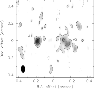
Figure 16: 43 GHz continuum image of sources A1 and A2. The synthesized beam is $86\times 47$ mas at P.A. 2^∘, shown at bottom left. Contours are spaced at approximately 2$\sigma$ intervals of 0.25 mJy beam^-1.

The position of A2 relative to B has remained constant over the past 17 years, exhibiting no residual proper motion that might be expected if A1 and A2 were part of a binary system with $M_{\rm A1}\sim M_{\rm A2}$, or if they were the oppositely-directed lobes of a precessing radio jet. The centimeter radio emission from A2 therefore probably pinpoints the location of a protostar. Indeed, when observed at the highest resolution available at 43 GHz, A2 appears to be bipolar with a position angle $\sim 45^{\circ}$, aligned with the large-scale northeast–southwest outflow (Fig. 16). Thus A2 is probably the driving source of this flow.

The source of the ionization in low luminosity protostars is generally thought to be the result of shocks: either accretion shocks very close to the protostar (e.g., Neufeld & Hollenbach 1996; Shang et al. 2004), or shocks in an otherwise neutral wind (Curiel, Cantó, & Rodríguez 1987; Ghavamian & Hartigan 1998; González & Cantó 2002). In the case of source A2, these shocks are probably internal shocks in a jet, giving rise to the bipolar structure in Fig. 16. The case of A1 is more puzzling. The separation A1$-$A2 remains remarkably constant, even though their position angle changes dramatically. This would suggest a physical association of these two sources, but even though A1 and A2 have comparable radio flux densities, A2 does not exhibit any reflex motion as a result of a gravitational interaction — the 3$\sigma$ upper limit to its motion relative to source B is $4.5(D/{\rm 160~{}pc})$ km s^-1. If the mass of A1 were instead much lower than A2, and its motion relative to A2 is interpreted as rotation, then the linear fit to the position angle as a function of time shown in Fig. 6 would correspond to a rotation period of $162\pm 19$ yr. For a (projected) separation of 0.35^′′ [$56(D/{\rm 160~{}pc})$ AU] this would imply a mass of $6.5(D/{\rm 160~{}pc})^{3}M_{\odot}$ for the protostar at A2. This mass is comparable to the mass of the entire envelope, $\sim 5(D/{\rm 160~{}pc})^{2}M_{\odot}$ (e.g., Schöier et al. 2002), and is inconsistent with the low total luminosity of IRAS 16293$-$2422, $27(D/{\rm 160~{}pc})^{2}L_{\odot}$ (Mundy et al. 1986). Even assuming a distance of 120 pc we would find a mass for A2 of $2.7M_{\odot}$, an envelope mass of $\sim 3M_{\odot}$, and a luminosity of $15L_{\odot}$, which remains inconsistent. If A1 were in a highly elliptical orbit and observed at periastron the mass of A2 could be lowered a little, but A1 will be unbound for A2 masses lower than $3.3(D/{\rm 160~{}pc})^{3}M_{\odot}$. Furthermore, the probability of observing A1 at periastron for a highly elliptical orbit is very low. It is therefore very unlikely that the motion of A1 relative to A2 represents a gravitationally bound system.

The fact that the position angle of A1 relative to A2 has traversed the rather wide opening angle of the east–west outflow from IRAS 16293$-$2422 leads us instead to interpret A1 as the location of a shock interaction between the precessing jet or collimated wind responsible for this flow and nearby dense gas. The close association of A1 with the (probable) torsionally-excited methanol emission lends support to this picture. The origin of this flow is discussed further in Section 4.2.

The peak brightness temperatures ($T_{\rm B}$) for the radio emission from source A2 are $\sim 300$ K at 8 GHz, $\sim 160$ K at 22 GHz, and $\sim 100$ K at 43 GHz. For A1 they are $\sim 420$ K at 8 GHz, $\sim 190$ K, and $\sim 140$ K at 43 GHz. Assuming the emission at each frequency to be dominated by gas with $\tau\gtrsim 1$ at $T=10^{4}$ K, as indicated by the centimeter spectral index, these brightness temperatures can be used to estimate source solid angles from $\Omega_{\rm source}=\Omega_{\rm beam}\times(T_{\rm B}/10^{4}$ K), which can then be used to estimate the linear dimension of the emitting region. The brightness temperatures above therefore imply linear dimensions for the shocked emission at A2 of $\sim 6\times 10^{13}(D/{\rm 160~{}pc})$ cm at 8 GHz, $\sim 2\times 10^{13}(D/{\rm 160~{}pc})$ cm at 22 GHz, and $\sim 9\times 10^{12}(D/{\rm 160~{}pc})$ cm at 43 GHz. Similarly for A1, the linear dimensions are $\sim 8\times 10^{13}(D/{\rm 160~{}pc})$ cm at 8 GHz, $\sim 3\times 10^{13}(D/{\rm 160~{}pc})$ cm at 22 GHz, and $\sim 1\times 10^{13}(D/{\rm 160~{}pc})$ cm at 43 GHz. Individually, therefore, A1 and A2 do exhibit the decrease in source size as a function of frequency expected for partially optically-thick free-free emission.

4.1.2 Centimeter emission from source B

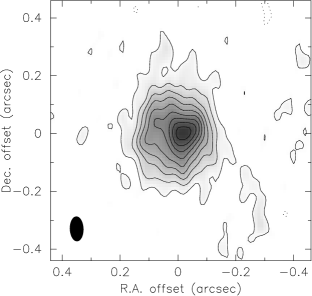
Figure 17: 43 GHz continuum image of source B. The synthesized beam and contours are as for Fig. 16.

Source B exhibits a centimeter radio spectrum consistent with being optically thick and thermal. The emission is much more centrally-peaked than is the case for source A, and formal Gaussian fits to the emission shown in Fig. 5 are for 15 GHz (1987.66) and 8 GHz (1989.05, 2002.41, and 2003.65) consistent with circular symmetry. At 22 GHz the emission has a position angle $\approx 22\pm 31^{\circ}$, and at 8 GHz, epoch 1994.30, the position angle is $\approx-10\pm 18^{\circ}$, consistent with that at 22 GHz, but both have large uncertainties. The deconvolved source size is $0.19^{\prime\prime}\times 0.15^{\prime\prime}$ at 22 GHz, and $0.16^{\prime\prime}\times 0.10^{\prime\prime}$ at 8 GHz. At 43 GHz the emission is resolved and the lower contours are approximately circular, with a peak slightly offset from the centroid of the outer contours (Fig. 17; see also Rodríguez et al. 2005). There are two possible origins for this emission: optically-thick free-free emission from ionized gas, or optically-thick dust emission. The trend in deconvolved source size with frequency is opposite to that expected for free-free emission, but is consistent with dust. The peak brightness temperatures observed are $\sim 160$ K at 8 GHz in a beam $0.35^{\prime\prime}\times 0.17^{\prime\prime}$, $\sim 350$ K at 22 GHz in a beam $0.194^{\prime\prime}\times 0.090^{\prime\prime}$ (see also Mundy et al. 1992), and $\sim 390$ K at 43 GHz in a beam $86\times 47$ mas. Thus temperatures of 390 K would appear to occur at a physical radius $\sim 5(D/{\rm 160~{}pc})$ AU, 350 K at $11(D/{\rm 160~{}pc})$ AU, and 160 K at $20(D/{\rm 160~{}pc})$ AU. This suggests a temperature gradient consistent with internal heating by a central protostar, although more detailed modelling is needed to establish the radial temperature profile.

In order for the $\nu^{2}$ dust spectrum of source B to extend to frequencies as low as 5 GHz either the dust column density must be very high, or the dust grains must be large, of order a few centimeter (e.g., Miyake & Nakagawa 1993). We cannot rule out a contribution to the 5 GHz emission from ionized gas, but consider the 8 GHz emission to be due to the same emission mechanism as at 15 GHz, 22 GHz, and 43 GHz. Given the high brightness temperature observed for the radio emission it is most likely that it is optically thick dust emission, although there may be large particles having opacities $\kappa_{\nu}\propto\nu^{\beta}$, with $\beta\sim 0$, as well. To estimate the mass of dust and gas for source B we assume a dust opacity suitable for particle densities $n_{\rm H}\sim 10^{8}$ cm^-3, for coagulated particles with no ice mantles, from Table 1, column 3, of Ossenkopf & Henning (1994). These authors give $\kappa=5.86$ cm² g^-1 at $\nu=230$ GHz, and from the lowest frequencies given in their Table 1, we find $\beta=1.1$, which we use to extrapolate to lower frequencies. Including a gas to dust ratio, $M_{\rm g}/M_{\rm d}=100$, we find $\kappa_{\rm 8~{}GHz}\sim 1.5\times 10^{-3}$ cm² g^-1 and $\kappa_{\rm 43~{}GHz}\sim 9.3\times 10^{-3}$ cm² g^-1, where $\kappa_{\rm 8~{}GHz}$ and $\kappa_{\rm 43~{}GHz}$ are now per gram of gas plus dust. Thus in order for the 8 GHz emission to be optically-thick ($\tau\sim\kappa N_{\rm H}m_{\rm H}\mu\sim 1$, where $N_{\rm H}$ is the column density of hydrogen atoms, $m_{\rm H}$ is the mass of a hydrogen atom, and $\mu\approx 1.36$ is the ratio of total gas mass to hydrogen mass: Hildebrand 1983), a particle column density $N_{\rm H}\sim 3\times 10^{26}$ cm^-2 is needed. For the 43 GHz emission to be optically-thick, $N_{\rm H}\sim 5\times 10^{25}$ cm^-2 is needed.

The deconvolved source size at 8 GHz corresponds to a radius $r\sim 11(D/{\rm 160~{}pc})$ AU, implying a total mass for a uniform source of $M=\pi r^{2}N_{\rm H}m_{\rm H}\mu\sim 0.03(D/{\rm 160~{}pc})^{2}M_{\odot}$. If the column density has a steeper radial dependence, for example $N_{\rm H}\propto r^{-3/2}$ as expected for an accretion disk, then the total mass may somewhat higher, $\sim 0.12(D/{\rm 160~{}pc})^{2}M_{\odot}$. At 43 GHz the emission extends out to radii of 0.2^′′ [$32(D/{\rm 160~{}pc})$ AU], with the lowest contour in Fig. 17 corresponding to a brightness temperature of 40 K. A similar calculation for the 43 GHz emission produces a total mass for a uniform source of $\sim 0.04(D/{\rm 160~{}pc})^{2}M_{\odot}$ at 43 GHz, and $\sim 0.16(D/{\rm 160~{}pc})^{2}M_{\odot}$ for a column density proportional to $r^{-3/2}$. Now, for a disk with surface density $\Sigma\propto r^{-p}$, $p>0$, it can easily be shown that the radius at which $\tau=1$ is proportional to $\nu^{\beta/p}$. The size of the 8 GHz emission compared with that at 43 GHz would suggest $\beta/p\sim 0.6$, similar to that expected for a disk model with $\beta\sim 1$ and $p\sim 3/2$. Note that although the emissivity of dust is highly uncertain at centimeter wavelengths, these masses are nevertheless reasonable, and can account for the observed radio emission. We do not find a mass as high as that derived using a similar surface density distribution by Rodríguez et al. (2005) of 0.5–0.7 $(D/{\rm 160~{}pc})^{2}M_{\odot}$, which we attribute to a different assumed dust opacity.

We now take the peak brightness temperatures per beam, and the physical size scale of the corresponding beam at the source, to estimate the contribution of source B to the total luminosity for IRAS 16293$-$2422 derived from the spectral energy distribution of $27(D/{\rm 160~{}pc})^{2}L_{\odot}$ (Mundy et al. 1986). In an exact 1D radiative transfer solution for dusty protostellar envelopes, for the case where the radiation field is optically-thick in the far-infrared, Preibisch, Sonnhalter, & Yorke (1995) show that in the temperature range $\sim 150$–400 K the radiation temperature is approximately 25% higher than that expected from simply assuming $L=4\pi r^{2}\sigma T^{4}$. We therefore estimate the luminosity of source B from the observed brightness temperatures using $L=4\pi r^{2}\sigma(0.8T)^{4}$, and find that $T=160$ K at radius $r\sim 20(D/{\rm 160~{}pc})$ AU gives $L\sim 4.4(D/{\rm 160~{}pc})^{2}L_{\odot}$; $T=350$ K at $r\sim 11(D/{\rm 160~{}pc})$ AU gives $L\sim 31(D/{\rm 160~{}pc})^{2}L_{\odot}$; and $T=390$ K at $r\sim 5(D/{\rm 160~{}pc})$ AU gives $L\sim 10(D/{\rm 160~{}pc})^{2}L_{\odot}$. Although these numbers are only rough estimates, the brightness temperature derived from the 22 GHz emission in particular indicates that source B is responsible for a least half the total luminosity, and indeed may suggest that the radiation field probably has to be anisotropic. One possibility that can reconcile this luminosity estimate and the observed morphology of the radio source is that the emission arises from a face-on disk. We can therefore conclusively rule out the possibility that source B is a low-luminosity, young T Tauri star, as has been suggested by Stark et al. (2004).

4.1.3 Submillimeter emission from A and B

At $\nu>100$ GHz the spectra of sources A and B are consistent with optically-thin dust emission with $\beta\gtrsim 0.8$ for source A, and $\beta\gtrsim 0.4$ for source B. As described above in Section 3 the different $u$-$v$ coverage for each of the millimeter and submillimeter data points in Fig. 2 make the derivation of the spectral index rather more uncertain than the errors quoted in the figure. However, the overall spectrum of the entire region is well-fitted by a single-temperature greybody with $T_{\rm dust}=40\pm 1$ K and $\beta=1.6$ (Stark et al. 2004), which for optically-thin emission gives a 300 to 110 GHz spectral index of $\alpha=3.48$, somewhat steeper than that observed for the individual sources in Fig. 2. The brightness temperatures of the submillimeter emission obtained from the image shown in Fig. 3 restored with a normal CLEAN beam of $1.23^{\prime\prime}\times 0.64^{\prime\prime}$ at P.A. $10^{\circ}$ (instead of a circular 0.4^′′ beam) are 21 K for source A, and 38 K for source B. Since the temperature of dust in the envelope on these scales is probably less than 100 K, the submillimeter dust emission from the envelope clearly has significant optical depth at $\sim 150$ AU, that may account for the shallower spectral index of the emission detected by the interferometers compared with the overall envelope.

A striking feature of the dust continuum emission from source A is that even on subarcsecond size scales there is little evidence of flattened structures that one might call a “disk.” For the case of the collapse of a slowly rotating, singular isothermal sphere, the centrifugal radius is given by $R=\Omega^{2}G^{3}M^{3}/16a^{8}$, where $\Omega$ is the angular velocity of the cloud, $M$ is the central mass, and $a$ is the isothermal sound speed (Terebey, Shu, & Cassen 1984; hereafter TSC). The kinematics of the surrounding cloud core have been examined by Zhou (1995) and Narayanan et al. (1998) in terms of the TSC model, for which the best fits give $\Omega\approx 4\times 10^{-13}$ s^-1, and $a\approx 0.5$ km s^-1. For a 1 $M_{\odot}$ central object this gives $R\sim 40$ AU ($\sim 0.3^{\prime\prime}$). Note that there is a very steep dependence of $R$ on $a$, and the cloud is not isothermal. Nevertheless, this calculation may explain why, even with the resolution available with the SMA, the dust emission does not look “disk-like”; any disk remains below the resolution limit of the current submillimeter data.

The location of Aa almost exactly between the radio sources A1 and A2 implies either that there is a protostar at this position, or that the flux ratio of any dust emission associated with A1 and A2 is close to unity. The interpretation of A1 as shock-ionized gas resulting from a wind or jet impacting dense gas would suggest that A1 should also be the location of significant dust emission; if so, a model where A1 and A2 are both sources of submillimeter emission, with roughly equal fluxes, would seem to explain the data best. Higher resolution submillimeter observations are clearly needed to establish whether there is really a separate source at the position of Aa.

In order to obtain lower limits on the masses of the compact components listed in Table 3 we assume a dust opacity $\kappa_{\rm 300~{}GHz}\sim 1.5$ cm² g^-1 appropriate for dust grains with ice mantles from Ossenkopf & Henning (1994, Table 1), $M_{\rm g}/M_{\rm d}=100$, and $T_{\rm dust}=40$ K. The particle column density needed for $\tau\sim 1$ is then $N_{\rm H}\sim 3\times 10^{25}$ cm^-2, and the corresponding masses for a uniform source are $M_{\rm Aa}\sim 0.14(D/{\rm 160~{}pc})^{2}M_{\odot}$, $M_{\rm Ab}\sim 0.04(D/{\rm 160~{}pc})^{2}M_{\odot}$, and $M_{\rm B}\sim 0.23(D/{\rm 160~{}pc})^{2}M_{\odot}$. Note that extrapolating the centimeter wavelength emission from source B to 300 GHz (Fig. 2) suggests a contribution to the 300 GHz flux from the optically-thick disk of $\sim 1.4$ Jy, which is $\sim 50$% of the compact emission from Table 3. Assuming $p=3/2$ so that the mass of the disk is $\sim 0.16(D/{\rm 160~{}pc})^{2}M_{\odot}$, the contribution from the envelope is then $\sim 0.11(D/{\rm 160~{}pc})^{2}M_{\odot}$, and the total is $\sim 0.27(D/{\rm 160~{}pc})^{2}M_{\odot}$, similar to the value obtained for a uniform source with a lower overall value of $\kappa$.

4.2 Relationship between the radio sources and the large-scale outflows

At least two outflows have been identified originating from the vicinity of IRAS 16293$-$2422, one oriented NE–SW with its redshifted lobe to the northeast, and the other approximately E–W with its redshifted lobe to the west (Mizuno et al. 1990; Stark et al. 2004). Mizuno et al. (1990) also detect a low-velocity, unipolar blueshifted lobe extending 10 arcmin to the east, which Stark et al. suggest is just an extension of the E–W flow. The redshifted counterpart of this blue lobe has probably already broken out of the molecular cloud to the west. The NE–SW flow is well-collimated, and centered on source A. Estimates of the inclination to the plane of the sky for this flow range from 30–45^∘ (Hirano et al. 2001) to 65^∘ (Stark et al. 2004). There is, however, considerable low-velocity red and blueshifted emission spatially coincident with the blue and redshifted lobes of this flow respectively in the maps of Stark et al., suggesting that an inclination closer to the plane of the sky than 65^∘ may be most appropriate. We have identified the radio source A2 as the source of this flow, based on its apparent bipolar morphology aligned with the molecular outflow.

The red and blue peaks of the E–W flow are centered somewhat to the north of source A, but the emission is messy, and at low velocities, close to IRAS 16293$-$2422, the contours in the maps of Stark et al. (2004) are in fact also centered close to source A. The E–W flow exhibits a larger opening angle than the NE–SW flow. The orientation of the E–W flow is such that its interaction with I16293E, a nearby and possibly starless dark cloud 1.5^′ to the east of IRAS 16293$-$2422, has disrupted the flow, as it streams around the edges of this cloud. These features led Stark et al. to suggest that the E–W flow is a fossil flow driven by source B. Such an interpretation would imply that source B is older than source A, and that source B is a low-luminosity pre-main sequence star. This would seem to be in contradiction with the observations of source B which indicate some of the same features as deeply-embedded class 0 protostars, such as the presence of some of the same hot core molecules as are observed for source A, and with the high luminosity implied by the brightness temperatures derived from the radio emission in Section 4.1. Furthermore, the narrow linewidths associated with source B would suggest instead that source B is younger than source A (a conclusion also reached by Wootten 1989).

Copious water masers are associated with various shocks at sources Aa/A1/A2, and exhibit expansion proper motions of $\sim 65(D/{\rm 160~{}pc})$ km s^-1 in the plane of the sky (Wootten et al. 1999), considerably higher than the radial velocities observed in the molecular component of the outflows on larger scales, of 10–20 km s^-1. Furthermore, the motion of A1, interpreted above as tracing the location of the shock interaction of dense gas with a precessing jet, makes the origin of this jet a good candidate for explaining some of the features of the E–W outflow, such as its wide opening angle, its apparent recollimation on the far side of I16293E (Stark et al. 2004), and the collimated unipolar blueshifted flow (Mizuno et al. 1990): the apparent recollimation and the unipolar flow would be interpreted as directions of lower density that have been evacuated during previous epochs of the jet passing in these directions.

So, where is the driving source of this precessing jet? The rate at which the jet is precessing may provide a clue. The precession of jets has been inferred for some time now to explain S-shaped optical jets and Herbig-Haro flows (e.g., Bally & Devine 1994; Schwartz & Greene 1999), and the presence of multiple bow shocks in molecular outflows such as RNO 43 and L1157 (Bence, Richer, & Padman 1996; Gueth et al. 1997). However, such a dramatic change in position angle over a relatively short time baseline, such as that presented here for IRAS 16293$-$2422, has not been observed directly before. Various authors have investigated the possibility that the tidal interaction between a star with a circumstellar disk and a binary companion in an orbit misaligned with the disk might cause jet precession, assuming the jet to originate in the inner regions of the disk (e.g., Terquem et al. 1999; Bate et al. 2000). In these scenarios, the disk precesses about the orbital axis with a period $P_{\rm prec}\sim 20P_{\rm orb}$, where $P_{\rm orb}$ is the orbital period. On top of this precession, the disk might wobble in response to the torque exerted on the disk in the direction aligning it with the binary orbit, with a wobble period $\sim P_{\rm orb}/2$ (Bate et al. 2000).

If the slight curvature in the observed rate of change of position angle as a function of time in Fig. 6 is interpreted as precession, the precession (or wobble) period of the jet is $\lesssim 100$ yr. Assuming the wobble to be induced by a binary system with period $\lesssim 200$ yr the binary separation would have to be $\lesssim 22$ AU (0.14^′′) for the wobble described above, or $\lesssim 2$ AU for precession, assuming a total stellar mass of 1 $M_{\odot}$. Since we have already established that the radio emission from A2 is probably associated with a protostar, we therefore look to a second source in the vicinity of A2, in an inclined orbit to A2, as the origin of the precessing jet that drives the E–W molecular outflow. We note that, although Aa is not yet established as a separate source rather than the centroid of submillimeter emission from A1 and A2, the separation between A2 and Aa is similar to the binary separation required if Aa were the origin of the E–W outflow and the precessing jet. The new submillimeter source Ab has a projected separation from Aa of 0.64^′′, or 102 AU. Assuming a circular orbit this would result in an orbital period $\sim 10^{3}$ yr, and a wobble period $\sim 500$ yr, clearly too long to account for the change in position angle of the centimeter radio emission.

The total CO momentum rate in the E–W flow is $\sim 4\times 10^{-4}$ $M_{\odot}$ km s^-1 yr^-1 (including the unipolar blueshifted lobs), and that of the NE–SW flow is $\sim 1\times 10^{-4}$ $M_{\odot}$ km s^-1 yr^-1 (Mizuno et al. 1990). While there is large scatter in the observed correlations between 5 GHz radio emission and the CO momentum rate (Cabrit & Bertout 1992; Anglada 1995), these momentum rates are certainly sufficient to account for the radio emission in terms of shock ionization.

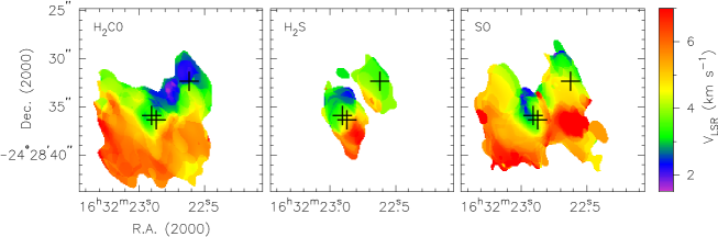
Figure 18: Intensity-weighted mean radial velocity for H₂CO, H₂S, and SO emission. The positions for sources Aa, Ab, and B from Table 3 are marked as crosses.

The passage of a jet with variable directions and inclinations to the plane of the sky also helps to explain the kinematics of the molecular gas on small scales close to source A. Fig. 18 shows the intensity-weighted mean velocity (first moment) images of the formaldehyde, H₂S, and SO emission. There is a clear velocity gradient that lies perpendicular to the NE–SW outflow, along a line connecting sources A and B, that has been investigated in a number of single-dish and interferometric studies and interpreted as rotation about an axis approximately aligned with this outflow (Mundy et al. 1986; Menten et al. 1987; Walker, Carlstrom, & Bieging 1993). However, the kinematics are complicated by emission from the outflows themselves, made all the more confusing because the dominant velocity gradients along the outflow directions are actually reversed from those of the large-scale, high-velocity CO emission.

Fig. 18 illustrates widespread redshifted formaldehyde emission to the south of source A, while the blueshifted emission lies predominantly to the northwest of A, along the axis joining A and B. This geometry is almost exactly the opposite of the kinematics in the CO outflows. For H₂S the emission is more localized around sources A and B, with B having a narrow linewidth, $\sim 1.6$ km s^-1, compared with $\sim 6$ km s^-1 for source A (Fig. 10). Across source B there is a shallow velocity gradient running NW–SE, while the velocity gradient associated with source A runs along the axis of the NE–SW outflow, but in the opposite sense from the higher velocity CO. The SO first moment image is similar to the H₂CO, but extends to higher velocities because of the higher signal-to-noise ratio in the stronger line. Two distinct axes can be defined for the principal kinematic features, one along the line joining sources Aa and Ab at P.A. 45^∘, aligned with the NE–SW outflow, and one perpendicular to this at P.A. 135^∘, along the line joining source A and source B, and aligned with the velocity gradient associated with the proposed rotation.

Figs. 19 and 20 show position-velocity (P–V) diagrams for cuts along P.A. 45^∘ aligned with the NE–SW outflow for sources A and B, and for a cut at P.A. 135^∘ along a line connecting sources A and B. The general agreement between the overall structure observed in the two species exhibiting extended emission, H₂CO and SO, is striking. There is, however, one noticeable difference: the formaldehyde is lacking emission close to the systemic velocity of the cloud, $\approx 4$ km s^-1, probably due to a combination of self-absorption by the cooler, outer envelope at these velocities, and the fact that the interferometer filters out much of the extended emission at the cloud velocity. Thus the apparent difference in $V_{\rm LSR}$ for sources A and B, with B exhibiting $V_{\rm LSR}\sim 3$ km s^-1 for H₂CO, is probably exacerbated by this problem. Indeed, for the H₂S and SO emission, which have much lower abundances in the outer envelope and so do not exhibit such self-absorption, the velocities of A and B are more similar. The velocity gradient along the axis connecting A and B no longer looks like rotation now that it is observed at such high spatial resolution. Rather, it is probably a combination of the spatial filtering and self-absorption at the cloud systemic velocity, and the enhancement of molecular emission in shocked clumps as the outflow interacts with the envelope.

Although overall the sense of the red and blueshifted emission from the high density tracers is in the opposite sense to that of the outflows, the cut along axis A–B, Fig. 20, does reveal the presence of a spatially compact, kinematic feature at source A (marked as a dashed line in that figure), with velocities extending $\pm 6$ km s^-1 from the systemic velocity within $\pm 1^{\prime\prime}$ of the continuum source, and with the same velocity sense as the large-scale CO outflows. This feature is masked by the bright, extended emission in the first moment maps, but does lend support to the idea that the more energetic, E–W flow, is driven by source A. However, none of the P–V diagrams exhibit the “typical” outflow signatures observed in, e.g., CO emission, because of the confusing effects of abundance enhancements in local shocks.

Fig. 19 shows that at P.A. 45^∘, along the direction of the NE–SW outflow, both the H₂CO and SO emission from source A is clumpy, and is extended particularly at velocities close to the systemic velocity of the cloud, 4 km s^-1. The velocity gradient of redshifted emission toward the southwest (negative position offsets) to blueshifted in the northeast is predominantly within $\pm 1^{\prime\prime}$ of the continuum peak, and the linear feature marked by the dashed line is typical of the P–V diagrams resulting from rotating protostellar disks (Richer & Padman 1991). If interpreted as rotation, the observed velocity gradient would correspond to a total central mass for source A of $\sim 1.5$–2 $M_{\odot}$.

The velocity gradient at source B is harder to interpret, because only the H₂CO emission peaks close to the continuum source, and this suffers from the self-absorption and spatial filtering at the velocity of the cloud described above.

4.3 Relationship between the hot core and the continuum sources

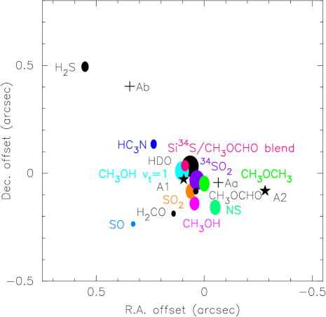
Figure 21: Location of the integrated emission peaks for the molecular species detected from IRAS 16293$-$2422 (ellipses) and the continuum sources Aa, Ab (crosses), A1, and A2 (stars). The ellipse semi-axes represent the 1$\sigma$ uncertainties in the positions. R.A. and dec. offsets are relative to the peak in Fig. 1.

The emission from species more commonly associated with hot cores in massive star-forming regions is predominantly located close to source A. However, the molecular emission is not coincident with either of the submillimeter continuum peaks. Fig. 21 plots the position of the peak in the integrated emission from each species as $\pm 1\sigma$ error ellipses, and shows that all the molecular species peak to the southeast of a line joining sources Aa and Ab. A comparison with Fig. 5 shows that many of the species, but especially the emission from the high-energy transition of torsionally-excited methanol, lies in the direction of the shock-ionized radio emission at source A1, and lends support to our interpretation of A1 as the location of a clump of very dense gas into which the jet driving the E–W outflow is ploughing. Furthermore, the location of the molecular peaks are all approximately aligned with the directions through which the jet has passed over the last 20 years. Thus we infer that the passage of the jet, and its shock interaction with the dense gas east of Aa, is responsible for enhancing the abundances of many species at this location, and providing the high excitation temperatures.

The four molecules that peak somewhat to the south of Aa, i.e., SO, H₂CO, CH₃OH, and NS, are all transitions having $E_{\rm upper}<100$ K, and the two of these furthest from Aa, SO and H₂CO, have contributions from extended emission. Most of the high-energy transitions originate directly east of Aa, close to the shock at A1, although HC₃N and H₂S appear at somewhat larger distances along the direction of the NE–SW outflow. Note also that those molecules detected in emission with $T_{\rm rot}\lesssim 90$ K (H₂S, H₂CO, SO and CH₃OH; Table 5) lie at some distance from A1. The remaining molecules (excluding NS, for which $T_{\rm rot}$ has not been measured) have $T_{\rm rot}\gtrsim 90$ K, and are mostly within 0.1^′′ [$16(D/{\rm 160~{}pc})$ AU] of A1. The one exception is HC₃N, which has a high derived $T_{\rm rot}$ and yet lies 0.2^′′ from A1 towards the northeast. However, the uncertainty in its $T_{\rm rot}$ is very large, and is still consistent with being less than 90 K. Further measurements of intermediate energy transitions are needed to constrain better the excitation and origin of the HC₃N emission from IRAS 16293$-$2422.

4.4 The unambiguous detection of infall

The detection of infall due to gravitational collapse in star forming regions using molecular emission lines can be confused and complicated by other motions in the gas, such as rotation and outflow. The best examples to date are for sources with simple outflow geometries, for which the contributions to the kinematics from outflow and rotation can be quantified or separated (e.g., B335: Zhou et al. 1993). Claims of the detection of infall for IRAS 16293$-$2422 have been more controversial, because of the other velocity gradients across the core and the presence of multiple outflows (Walker et al. 1986; Menten et al. 1987; Narayanan et al. 1998). Furthermore, most of the molecular emission line studies are generally based on data from single-dish telescopes, which trace the outer envelope on scales of a few $\times 1000$ AU, and not material collapsing onto the protostar/accretion disk system itself.

The high brightness temperature of the dust continuum emission associated with sources A and B in IRAS 16293$-$2422 raises the exciting possibility of using the compact submillimeter emission from the dust disks as a background source against which to detect redshifted absorption, which would indicate infall on the size scale of the disk itself. Ultimately this is the only unambiguous way of establishing whether gas is infalling because the absorbing material must be located in front of the protostar, and any blueshifted emission or absorption must be outflow, while material in rotation about the central object will have motion perpendicular to the line of sight, contributing only to absorption at the systemic velocity. It is important to use a high-dipole moment molecule and a transition that is likely to have $T_{\rm ex}<T_{\rm B,~{}dust}$ for such an experiment, in order to probe the inner parts of the infall envelope. We have already shown the molecules such as DNO, present in the cool, outer envelope of IRAS 16293$-$2422, can be observed in absorption against the dust emission (Fig. 11). Di Francesco et al. (2001) show that the $3_{1,2}$$-$$2_{1,1}$ transition of formaldehyde at 225.7 GHz is detected with an inverse P Cygni profile towards the dust emission from the low-mass protostar NGC 1333 IRAS4, and similar profiles for various transitions of ammonia and other molecules have been observed against the free-free continuum emission from HII regions (e.g., Zhang & Ho 1997; Zhang, Ho, & Ohashi 1998). The best candidate transitions for tracing the inner envelope in our data cube are those of formaldehyde and SO, but the formaldehyde is unfortunately blended with methyl formate on the redshifted side of the line. We therefore use SO to investigate the possibility of detecting collapse in the envelope on size scales of the background dust emission. The chemical models of Schoier et al. (2002) and Doty et al. (2004) suggest high SO abundances only at small radii, and its excitation temperature also points towards an origin very close to the embedded protostars.

In Fig. 22 we show an image of the SO emission made using an AIPS robust weighting of 0 and excluding baselines shorter than 55 k$\lambda$, in order to filter out the extended envelope and isolate compact emission and absorption features. The emission associated with the hot core at source A is clear, as is absorption against the compact dust emission at source B. The spectrum of this absorption feature is also plotted. There is significant absorption extending $\sim 5$ km s^-1 both to the redshifted and blueshifted sides of the systemic velocity of 4 km s^-1. The blueshifted absorption must be associated with low-velocity outflow from source B (perhaps its outflow is in the earliest phase of punching its way out of the surrounding infall envelope), while the redshifted absorption must be due to envelope material infalling onto the accretion disk. The rms noise per channel in the spectrum is 0.5 Jy beam^-1, so the significance of the absorption feature in any one channel is marginal. However, reshifted absorption is detected in at least seven consecutive channels, making this a 5-$\sigma$ detection. Unfortunately this signal-to-noise ratio is insufficient to enable detailed modelling of the infall density and velocity profiles. However, the infall velocity ($V_{\rm inf}=\sqrt{2GM/r}$) for a 1 $M_{\odot}$ central star would suggest that the material responsible for this absorption is as close as 70 AU to the disk.

4.5 Conclusions

We have combined SMA data with archival VLA data to establish the relationship between the submillimeter and centimeter radio continuum sources, emission from hot core molecules, and the molecular outflows from the class 0 protostar IRAS 16293$-$2422. The overall proper motion of sources A and B originally noted by Loinard (2002) based on two epochs of 8 GHz data are now confirmed by other epochs and measurements at frequencies from 5 to 43 GHz. Most of this motion is that associated with the $\rho$ Ophiuchi molecular cloud, but there is also a significant relative motion of the centimeter radio sources A1 and A2, which excludes the possibility that these two sources are gravitationally bound unless A1 is in a highly eccentric orbit and is observed at periastron, the probability of which is low.

Sources A and B are separated by only 5.2^′′ [$830(D/{\rm 160~{}pc})$ AU], yet their properties differ dramatically. Source B is a single source at all frequencies observed to date, the highest resolution being 43 GHz with a beam $86\times 47$ mas, or $14\times 7.5$ AU. The continuum emission originates from optically-thick dust even at a frequency of 8 GHz, and exhibits brightness temperatures of 350–400 K on size scales of 5–10 AU. Source B is responsible for at least half the total luminosity of IRAS 16293$-$2422. The molecular emission from source B exhibits narrow line widths, with no sign of outflow. Combined with its high luminosity (which is presumably dominated by accretion) this suggests that source B may not even have begun a phase of significant mass loss yet.

We show that source A, on the other hand, probably comprises three stellar components. One is the centimeter radio source A2, which we identify as the driving source of the large-scale NE–SW molecular outflow. The second is an as-yet unidentified companion to A2 which drives a precessing jet responsible for shock-ionized centimeter emission at A1. The strongest submillimeter continuum emission from source A, denoted Aa, peaks between the radio sources A1 and A2, but the resolution of the SMA is insufficient to tell whether this marks the position of the companion to A2, or the centroid of submillimeter emission from A1 and A2. We suggest that this companion is responsible for the large-scale east–west molecular outflow, which is messy and has a wider opening angle than the NE–SW flow, all of which can be explained by a variable jet direction. Finally, we also identify a new submillimeter source 0.64^′′ away from Aa, which we denote Ab. This source is too far from Aa to be responsible for the precession of the jet. Most of the molecular emission originates from source A, and the overall kinematics of the envelope are in the opposite sense to that of the outflows, with redshifted emission to the south, and blueshifted emission to the north. There is, however, one compact kinematic feature centered on source A that is similar to the large-scale east–west outflow, confirming this as its origin.

IRAS 16293$-$2422 is one of only a handful of low-mass protostars which exhibits emission from molecules more commonly associated with hot cores in regions of massive star formation. We show that in this low-mass source the emission from these molecules is coincident with the shock at A1. The abundances derived from the submillimeter emission indicate significant local enhancements over those expected for a low-mass protostar for many species, but especially those typically thought to trace shocks such as the sulphur-bearing molecules SO and SO₂. Our results highlight the key role of shocks in explaining the nature of hot cores, and demonstrate the importance of high-resolution imaging at submillimeter wavelengths with the SMA in pinning down rotation diagrams using high-energy transitions.

Finally, we discuss the possibility of using optically-thick dust emission from accretion disks as a background source against which to detect infall in the surrounding envelope. The advantage of using compact dust emission instead of the usual technique of using a molecular emission line as the background source is that the absorption must be on the physical size scale of the disk itself, and by choosing an appropriate molecular transition for the absorption it is possible to isolate the kinematics of infalling gas in the inner envelope, without confusion from other emission components such as outflow. When measured against the dust continuum any blueshifted absorption must be outflow, rotation will be at the systemic velocity, and redshifted absorption can be unambiguously identified as infall. By excluding short baselines from the SMA data we detect redshifted absorption of SO ($7_{7}$$-$$6_{6}$) against source B extending 5 km s^-1 from the systemic $V_{\rm LSR}$. Unfortunately the signal-to-noise ratio is not sufficient to allow a detailed analysis of the infall kinematics of IRAS 16293$-$2422, but clearly this will be a possibility in the future.

Figure 2: Continuum spectra of sources A and B compiled from the SMA and VLA data (Table 2), including data from the literature at 110 and 230 GHz (Bottinelli et al. 2004) and 354 GHz (Kuan et al. 2004). The lines show best-fit power laws, $F_{\nu}\propto\nu^{\alpha}$, to the data for $\nu<100$ GHz (solid) and $\nu>100$ GHz (dot-dash).

Figure 4: Left: the proper motion of source B, plotted as offsets from the submillimeter position given in Table 3. Center: the motion of radio source A2 relative to source B, as a function of time. Right: the separation A1$-$A2 as a function of time.

Figure 6: Projected separation $|$A1$-$A2$|$ (left) and the position angle of the vector joining A2 and A1 (right) as a function of time. The lines represent the best linear (dot–dash) and quadratic (dotted) fits to the position angle data. The linear fit gives $2.22\pm 0.26$ deg yr^-1.

Figure 7: Integrated fluxes for sources A (left) and B (right) as a function of time.

Figure 13: Rotation diagrams for the organic species detected; data from this work are marked as filled stars. Supplementary CH₃OCH₃ data come from Cazaux et al. (2003), and the upper limits are from van Dishoeck et al. (1995). The dot-dash line is for $T_{\rm rot}=95$ K. Supplementary HC₃N data are from Suzuki et al. (1992), van Dishoeck et al. (1995), and Schöier et al. (2002). The dot-dash line is for $T_{\rm rot}=320$ K, and does not include the low energy $J$=5$-$4 line in the fit.

Figure 14: Rotation diagrams for the sulphur-bearing species detected; data from this work are marked as filled stars. Supplementary SO₂ data come from Blake et al. (1994), and the dot-dash line is for $T_{\rm rot}=135$ K. Supplementary H₂S data come from Blake et al. and Wakelam et al. (2004b), and the dot-dash line is for $T_{\rm rot}=60$ K.

Figure 15: Rotation diagram for HDO; data from this work are marked as filled stars. Supplementary data are from van Dishoeck et al. (1995), Stark et al. (2004), and Parise et al. (2004b), and the dot-dash line is for $T_{\rm rot}=236$ K. The low point at $E_{\rm upper}/k=157$ K is not included in the fit, for the reasons described in the text.

Figure 19: Position-velocity diagrams for cuts at P.A. = 45^∘ through source A (top panels) and source B (bottom panels). Contours are linearly spaced at 0.65 Jy beam^-1. The dashed line in the panels for source A shows the velocity gradient passing through the position of the continuum peak at the systemic $V_{\rm LSR}=4$ km s^-1.

Figure 20: Position-velocity diagrams for a cut at P.A. = 135^∘ through a line joining sources A and B. Contours are as in Fig. 19. The dashed line denotes the kinematic feature described in the text having the velocity gradient with the same sense as the large-scale CO outflow. This kinematic feature passes through the position of the continuum peak at source A and the systemic $V_{\rm LSR}=4$ km s^-1. The dot-dash line shows the position of the continuum peak at source B.

Figure 22: Left: image of the integrated SO ($7_{7}$$-$$6_{6}$) emission obtained using an AIPS robust weighting of 0 and excluding baselines shorter than 55 k$\lambda$. The resulting CLEAN beam is $1.57^{\prime\prime}\times 0.72^{\prime\prime}$ at P.A. 22, shown in the bottom left corner. Contours are evenly spaced at intervals of 3.7 Jy km s^-1. Right: spectrum of the absorption feature at source B, with the systemic $V_{\rm LSR}$ of 4 km s^-1 indicated by the dot-dash line. The rms noise per channel is 0.5 Jy beam^-1.

Table 1: Summary of VLA continuum archive data.

Date	$\nu$ (GHz)	Configuration	Reference
1986 Jul. 03	04.86	BnA	Wootten (1989)
1987 Aug. 30	14.94	A	Wootten (1989)
1987 Oct. 25	01.49	BnA	$\cdots$
1987 Nov. 01	01.49	BnA	$\cdots$
1988 Mar. 27	14.94	C	Estalella et al. (1991)
1988 Mar. 27	22.46	C	Estalella et al. (1991)
1988 Jul. 17	14.94	D	Estalella et al. (1991)
1988 Aug. 10	14.94	D	Estalella et al. (1991)
1988 Aug. 20	14.94	D	Estalella et al. (1991)
1989 Jan. 20	08.44	A	Mundy et al. (1992)
1989 Jan. 20	22.46	A	Mundy et al. (1992)
1989 Apr. 19	14.94	B	$\cdots$
1992 Apr. 30	08.44	C	$\cdots$
1992 Apr. 30	14.94	C	$\cdots$
1992 Apr. 30	22.46	C	$\cdots$
1994 Apr. 14	08.44	A	Loinard (2002)
1994 Apr. 15	08.44	A	Loinard (2002)
1994 Apr. 22	08.44	A	Loinard (2002)
1994 May 20	08.44	BnA	Loinard (2002)
1998 Jun. 16	22.25	BnA	$\cdots$
2002 May 30	08.46	BnA	$\cdots$
2003 Jun. 22	43.34	A	Rodríguez et al. (2005)
2003 Aug. 26	08.46	A	$\cdots$

Table 2: Integrated SMA and VLA continuum flux densities.

$\nu$ (GHz)	$F_{\nu}$, Source A (mJy)	$F_{\nu}$, Source B (mJy)
001.49	$1.32\pm 0.17$	$<0.32~{}(3\sigma)$
004.86	$2.81\pm 0.29$	$0.281\pm 0.048$
008.44	$3.17\pm 0.76$	$0.738\pm 0.089$
14.94	$4.66\pm 0.62$	$2.60\pm 0.21$
22.46	$5.00\pm 0.74$	$7.28\pm 1.20$
43.34	$8.7\pm 1.6$	$24.7\pm 2.5$0
305	$3460\pm 350$0	$3150\pm 320$0

Table 3: Positions and flux densities for compact components.

Source	R.A. (J2000)	Dec. (J2000)	$F_{\rm 305~{}GHz}$ (Jy)
Aa	$16^{\rm h}32^{\rm m}22\fs 8721\pm 0\fs 0010$	$-24^{\circ}28^{\prime}36\farcs 331\pm 0\farcs 018$	$\sim 1.6$
Ab	$16^{\rm h}32^{\rm m}22\fs 9060\pm 0\fs 0028$	$-24^{\circ}28^{\prime}35\farcs 885\pm 0\farcs 048$	$\sim 0.5$
B	$16^{\rm h}32^{\rm m}22\fs 6221\pm 0\fs 0004$	$-24^{\circ}28^{\prime}32\farcs 326\pm 0\farcs 009$	$\sim 2.7$

Table 4: Summary of all lines detected in the lower and upper sidebands for IRAS 16293$-$2422.

Molecule	Notation	Transition	Frequency (MHz)	$E_{\rm upper}$ (K)	$\int I_{\nu}dV$ (Jy km s-1)
CH3OCH3	$J_{K_{a},K_{c}}$	$5_{4,2}$$-$$4_{3,1}$ (AE)	299884.15	036.2	30.0$\pm$	6.7
		$5_{4,1}$$-$$4_{3,1}$ (EA)	299886.18	036.2	$\cdots$
		$5_{4,2}$$-$$4_{3,2}$ (EA)	299886.79	036.2	$\cdots$
		$5_{4,1}$$-$$4_{3,2}$ (AE)	299888.82	036.2	$\cdots$
		$5_{4,1}$$-$$4_{3,1}$ (EE)	299889.91	036.2	$\cdots$
		$5_{4,2}$$-$$4_{3,2}$ (EE)	299890.95	036.2	$\cdots$
		$5_{4,2}$$-$$4_{3,1}$ (AA)	299892.04	036.2	$\cdots$
		$5_{4,1}$$-$$4_{3,2}$ (AA)	299896.72	036.2	$\cdots$
		$8_{3,5}$$-$$7_{2,6}$ (AE)	299899.47	045.5	15.9$\pm$	4.0
		$8_{3,5}$$-$$7_{2,6}$ (EA)	299899.78	045.5	$\cdots$
		$8_{3,5}$$-$$7_{2,6}$ (EE)	299903.00	045.5	$\cdots$
		$8_{3,5}$$-$$7_{2,6}$ (AA)	299906.38	045.5	$\cdots$
CH3OCHO-A	$J_{K_{a},K_{c}}$	$24_{6,19}$$-$$23_{6,18}$	300063.94	202.8	blended
		$26_{3,24}$$-$$25_{3,23}$	300079.11	207.0	blended
		$26_{2,24}$$-$$25_{4,22}$	300134.83	207.0	blended
		$27_{1,26}$$-$$26_{2,25}$	300834.13	210.8	blended
		$27_{2,26}$$-$$26_{2,25}$	300835.70	210.8	blended
		$27_{1,26}$$-$$26_{1,25}$	300836.94	210.8	blended
		$27_{2,26}$$-$$26_{1,25}$	300838.52	210.8	blended
		$27_{3,25}$$-$$26_{3,24}$	310652.71	221.9	blended
		$27_{2,25}$$-$$26_{2,24}$	310686.06	221.9	blended
		$26_{3,23}$$-$$25_{3,22}$	310693.76	216.6	blended
		$28_{1,27}$$-$$27_{2,26}$	311416.28	225.7	blended
		$28_{2,27}$$-$$27_{2,26}$	311417.16	225.7	blended
		$28_{1,27}$$-$$27_{1,26}$	311417.86	225.7	blended
		$28_{2,27}$$-$$27_{1,26}$	311418.74	225.7	blended
		$25_{8,18}$$-$$24_{8,17}$	311641.97	235.5	blended
CH3OCHO-E	$J_{K_{a},K_{c}}$	$26_{5,22}$$-$$25_{5,21}$	300070.76	207.0	blended
		$26_{4,23}$$-$$25_{4,22}$	300126.62	207.0	blended
		$36_{7,30}$$-$$36_{5,32}$	300399.60	393.5	blended
		$36_{7,30}$$-$$36_{6,31}$	300399.90	393.5	blended
		$25_{5,20}$$-$$24_{5,19}$	300403.20	201.7	blended
		$36_{6,30}$$-$$36_{5,32}$	300408.10	393.5	blended
		$36_{6,30}$$-$$36_{6,31}$	300408.40	393.5	blended
		$27_{3,25}$$-$$26_{2,24}$	300829.09	210.8	blended
		$27_{2,25}$$-$$26_{2,24}$	300830.68	210.8	blended
		$27_{3,25}$$-$$26_{3,24}$	300831.93	210.8	blended
		$27_{2,25}$$-$$26_{3,24}$	300833.51	210.8	blended
		$27_{5,23}$$-$$26_{5,22}$	310644.51	221.9	blended
		$27_{4,24}$$-$$26_{4,23}$	310677.95	221.9	blended
		$26_{5,21}$$-$$25_{5,20}$	310684.19	216.6	blended
		$15_{5,10}$$-$$14_{4,11}$	311408.99	087.9	blended
		$28_{3,26}$$-$$27_{2,25}$	311411.35	225.7	blended
		$28_{2,26}$$-$$27_{2,25}$	311412.10	225.7	blended
		$28_{3,26}$$-$$27_{3,25}$	311412.70	225.7	blended
		$28_{2,26}$$-$$27_{3,25}$	311413.81	225.7	blended
		$25_{8,18}$$-$$24_{8,17}$	311637.10	235.5	blended
Si34S (?)	$J$	17$-$16	300066.00	129.7	blended
NS (${}^{2}\Pi_{1/2}$)	$J_{F}$	$6.5_{15/2}$$-$$5.5_{13/2}\,e$	300097.10	054.4	12.2$\pm$	2.8
		$6.5_{13/2}$$-$$5.5_{11/2}\,e$	300098.61	054.4	$\cdots$
		$6.5_{11/2}$$-$$5.5_{9/2}\,e$	300098.61	054.4	$\cdots$
HC3N	$J$	33$-$32	300159.65	245.1	30.5$\pm$	6.4
SO2	$J_{K_{a},K_{c}}$	$32_{3,29}$$-$$32_{2,30}$	300273.42	519.1	14.6$\pm$	3.5
H2S	$J_{K_{a},K_{c}}$	$3_{3,0}$$-$$3_{2,1}$	300505.56	169.0	77$\pm$	17
CH3OH $v_{t}=1$	$J_{K_{a},K_{c}}$	$16_{3,14}E$$-$$17_{4,14}E$	300763.40	732.4	4.0$\pm$	1.1
H2CO	$J_{K_{a},K_{c}}$	$4_{1,3}$$-$$3_{1,2}$	300836.64	047.9	397$\pm$	80
DNO	$J_{(K_{a},K_{c})_{F}}$	$4_{(1,3)_{3}}$$-$$3_{(1,2)_{3}}$	300952.30	049.5	absorption
		$4_{(1,3)_{5}}$$-$$3_{(1,2)_{4}}$	300955.14	049.5	$\cdots$
		$4_{(1,3)_{4}}$$-$$3_{(1,2)_{3}}$	300955.23	049.5	$\cdots$
		$4_{(1,3)_{3}}$$-$$3_{(1,2)_{2}}$	300955.33	049.5	$\cdots$
		$4_{(1,3)_{4}}$$-$$3_{(1,2)_{4}}$	300957.50	049.5	$\cdots$
SO	$N_{J}$	$7_{7}$$-$$6_{6}$	301286.12	071.0	582$\pm$	117
CH3OH	$J_{K_{a},K_{c}}$	$3_{1,3}E$$-$$2_{0,3}E$	310193.02	035.0	27.7$\pm$	6.1
HDO	$J_{K_{a},K_{c}}$	$5_{2,3}$$-$$5_{2,4}$	310533.29	437.7	12.0$\pm$	3.0
34SO2	$J_{K_{a},K_{c}}$	$17_{1,17}$$-$$16_{0,16}$	311485.38	135.6	7.6$\pm$	1.9
		$20_{4,16}$$-$$20_{3,17}$	311487.37	231.4	$\cdots$
Unidentified	$\cdots$	$\cdots$	300889.00	$\cdots$	$\cdots$
Unidentified	$\cdots$	$\cdots$	301077.00	$\cdots$	$\cdots$
Unidentified	$\cdots$	$\cdots$	310370.00	$\cdots$	$\cdots$
Unidentified	$\cdots$	$\cdots$	310505.00	$\cdots$	$\cdots$
Unidentified	$\cdots$	$\cdots$	310568.00	$\cdots$	$\cdots$
Unidentified	$\cdots$	$\cdots$	311023.00	$\cdots$	$\cdots$
Unidentified	$\cdots$	$\cdots$	311208.00	$\cdots$	$\cdots$
Unidentified	$\cdots$	$\cdots$	311313.00	$\cdots$	$\cdots$

Table 5: Rotation temperatures, emission sizes, column densities, and abundances for the molecules detected.

Molecule	Trot	Emission area	$N_{\rm mol}$		$N_{\rm mol}/N_{\rm H_{2}}$		$f_{\rm in}(X)$		$X_{\rm max}$
	(K)	(arcsec2)	(cm-2)
CH3OCH3	95$\pm$73	020.7	6.4$\times$	$10^{15}$	7.6$\times$	$10^{-8}$	$<4.0$$\times$	$10^{-8}$	3$\times$	$10^{-9}$
HC3N	320$\pm$300	011.2	1.6$\times$	$10^{14}$	1.0$\times$	$10^{-9}$	1.0$\times$	$10^{-9}$	3$\times$	$10^{-10}$
CH3OH	0850	010.5	1.7$\times$	$10^{16}$	9.4$\times$	$10^{-8}$	3.0$\times$	$10^{-7}$	1$\times$	$10^{-7}$
H2CO	0800	118.5	3.2$\times$	$10^{14}$	1.1$\times$	$10^{-7}$	6.0$\times$	$10^{-8}$	6$\times$	$10^{-8}$
NS	1000	007.2	2.3$\times$	$10^{14}$	6.4$\times$	$10^{-10}$	$\cdots$		$\cdots$
H2S	60$\pm$70	037.0	2.9$\times$	$10^{15}$	9.4$\times$	$10^{-8}$	9.0$\times$	$10^{-8}$	3$\times$	$10^{-9}$
SO	0800	132.2	1.2$\times$	$10^{15}$	5.0$\times$	$10^{-7}$	2.5$\times$	$10^{-7}$	4$\times$	$10^{-9}$
SO2	135$\pm$200	007.7	2.9$\times$	$10^{16}$	9.7$\times$	$10^{-8}$	1.0$\times$	$10^{-7}$	1$\times$	$10^{-8}$
34SO2	1350	003.3	1.7$\times$	$10^{15}$	1.3$\times$	$10^{-9}$	$\cdots$		$\cdots$
DNO	$\sim$15–20$\sim$	$\cdots$	$\sim 3$$\times$	$10^{15}$	$\sim 2$$\times$	$10^{-9}$	$\cdots$		$\cdots$
HDO	236$\pm$440	003.4	2.9$\times$	$10^{16}$	2.2$\times$	$10^{-8}$	$\cdots$		$\cdots$

References

- (1)
- (2) Anglada, G. 1995, Rev. Mex. Astr. Ap. (Ser. de Conf.), 1, 67
- (3) Baars, J. W. M., Genzel, R., Pauliny-Toth, I. I. K., & Witzel, A. 1977, A&A, 61, 99
- (4) Bally, J., & Devine, D. 1994, ApJ, 428, L65
- (5) Bate, M. R., Bonnell, I. A., Clarke, C. J., Lubow, S. H., Ogilvie, G. I., Pringle, J. E., & Tout, C. A. 2000, MNRAS, 317, 773
- (6) Bence, S. J., Richer, J. S., & Padman, R. 1996, MNRAS, 279, 866
- (7) Blake, G. A., van Dishoeck, E. F., Jansen, D. J., Groesbeck, T. D., & Mundy, L. G. 1994, ApJ, 428, 680
- (8) Bottinelli, S., Ceccarelli, C., Neri, R., Williams, J. P., Caux, E., Cazaux, S., Lefloch, B., Maret, S., & Tielens, A. G. G. M. 2004, ApJ, 617, L69
- (9) Briggs, D. S. 1995, PhD Thesis, New Mexico Institute of Mining and Technology
- (10) Cabrit, S., & Bertout, C. 1992, A&A, 261, 274
- (11) Caselli, P., Hasegawa, T. I., & Herbst, E. 1993, ApJ, 408, 548
- (12) Cazaux, S., Tielens, A. G. G. M., Ceccarelli, C., Castets, A., Wakelam, V., Caux, E., Parise, B., & Teyssier, D. 2003, ApJ, 593, L51
- (13) Ceccarelli, C., Castets, A., Loinard, L., Caux, E., & Tielens, A. G. G. M. 1998, A&A, 338, L43
- (14) Ceccarelli, C., Loinard, L., Castets, A., Tielens, A. G. G. M., & Caux, E. 2000, A&A, 357, L9
- (15) Ceccarelli, C., Loinard, L., Castets, A., Tielens, A. G. G. M., Caux, E., Lefloch, B., & Vastel, C. 2001, A&A, 372, 998
- (16) Charnley, S. B., Tielens, A. G. G. M., & Millar, T. J. 1992, ApJ, 399, L71
- (17) Chini, R. 1981, A&A, 99, 346
- (18) Curiel, S., Cantó, J., & Rodríguez, L. F. 1987, Rev. Mex. Astr. Ap., 14, 595
- (19) Curiel, S., Girart, J. M., Rodríguez, L. F., & Cantó, J. 2003, ApJ, 582, L109
- (20) Di Francesco, J., Myers, P. C., Wilner, D. J., Ohashi, N., & Mardones, D. 2001, ApJ, 562, 770
- (21) Doty, S. D., Schöier, F. L., & van Dishoeck, E. F. 2004, A&A, 418, 1021
- (22) Estalella, R., Anglada, G., Rodríguez, L. F., & Garay, G. 1991, ApJ, 371, 626
- (23) Garay, G., Ramírez, S., Rodríguez, L. F., Curiel, S., & Torrelles, J. M. 1996, ApJ, 459, 193
- (24) Ghavamian, P., & Hartigan, P. 1998, ApJ, 501, 687
- (25) Goldsmith, P. F., & Langer, W. D. 1999, ApJ, 517, 209
- (26) González, R. F., & Cantó, J. 2002, ApJ, 580, 459
- (27) Gueth, F., Guilloteau, S., Dutrey, A., & Bachiller, R. 1997, A&A, 323, 943
- (28) Hatchell, J., Thompson, M. A., Millar, T. J., & Macdonald, G. H. 1998, A&A, 338, 713
- (29) Hildebrand, R. H. 1983, QJRAS, 24, 267
- (30) Hirano, N., Mikami, H., Umemoto, T., Yamamoto, S., & Taniguchi, T. 2001, ApJ, 547, 899
- (31) Horn, A., Møllendal, H., Sekiguchi, O., Uggerud, E., Roberts, H., Herbst, E., Viggiano, A. A., & Fridgen, T. D. 2004, ApJ, 611, 605
- (32) Knude, J., & Høg, E. 1998, A&A, 338, 897
- (33) Kuan, Y.-J., et al. 2004, ApJ, 616, L27
- (34) Loinard, L. 2002, Rev. Mex. Astr. Ap., 38, 61
- (35) Loinard, L., Castets, A., Ceccarelli, C., Tielens, A. G. G. M., Faure, A., Caux, E., & Duvert, G. 2000, A&A, 359, 1169
- (36) Looney, L. W., Mundy, L. G., & Welch, W. J. 2000, ApJ, 529, 477
- (37) Menten, K. M., Serabyn, E., Güsten, R., & Wilson, T. L. 1987, A&A, 177, L57
- (38) Millar, T. J., Farquhar, P. R. A., & Willacy, K. 1997, A&AS, 121, 139
- (39) Millar, T. J., Herbst, E., & Charnley, S. B. 1991, ApJ, 369, 147
- (40) Minh, Y. C., Ziurys, L. M., Irvine, W. M., & McGonagle, D. 1990, ApJ, 360, 136
- (41) Miyake, K., & Nakagawa, Y. 1993, Icarus, 106, 20
- (42) Mizuno, A., Fukui, Y., Iwata, T., Nozawa, S., & Takano, T. 1990, ApJ, 356, 184
- (43) Müller, H. S. P., Thorwirth, S., Roth, D. A., & Winnewisser, G. 2001, A&A, 370, L49
- (44) Mundy, L. G., Wilking, B. A., & Myers, S. T. 1986, ApJ, 311, L75
- (45) Mundy, L. G., Wootten, H. A., Wilking, B. A., Blake, G. A., & Sargent, A. I. 1992, ApJ, 385, 306
- (46) Narayanan, G., Walker, C. K., & Buckley, H. D. 1998, ApJ, 496, 292
- (47) Neufeld, D. A., & Hollenbach, D. J. 1996, ApJ, 471, L45
- (48) Ossenkopf, V., & Henning, Th. 1994, A&A, 291, 943
- (49) Parise, B., Castets, A., Herbst, E., Caux, E., Ceccarelli, C., Mukhopadhyay, I., & Tielens, A. G. G. M. 2004a, A&A, 416, 159
- (50) Parise, B., et al. 2004b, A&A, in press
- (51) Patience, J., Ghez, A. M., Reid, I. N., & Matthews, K. 2002, AJ, 123, 1570
- (52) Pearson, T. J., & Readhead, A. C. S. 1984, ARA&A, 22, 97
- (53) Pickett, H. M., Poynter, R. L., Cohen, E. A., Delitsky, M. L., Pearson, J. C., & Müller, H. S. P. 1998, J. Quant. Spectrosc. & Rad. Transfer, 60, 883
- (54) Preibisch, T., Sonnhalter, C., & Yorke, H. W. 1995, A&A, 299, 144
- (55) Reynolds, S. P. 1986, ApJ, 304, 713
- (56) Richer, J. S., & Padman, R. 1991, MNRAS, 251, 707
- (57) Roberts, H., Fuller, G. A., Millar, T. J., Hatchell, J., & Buckle, J. V. 2002, A&A, 381, 1026
- (58) Rodríguez, L. F., Ho, P. T. P., Torrelles, J. M., Curiel, S., & Cantó, J. 1990, ApJ, 352, 645
- (59) Rodríguez, L. F., Loinard, L., D’Alessio, P., Wilner, D. J., & Ho, P. T. P. 2005, ApJ, in press
- (60) Schöier, F. L., Jørgensen, J. K., van Dishoeck, E. F., & Blake, G. A. 2002, A&A, 390, 1001
- (61) Schöier, F. L., Jørgensen, J. K., van Dishoeck, E. F., & Blake, G. A. 2004, A&A, 418, 185
- (62) Schwartz, R. D., & Greene, T. P. 1999, AJ, 117, 456
- (63) Serabyn, E., & Weisstein, E. W. 1995, ApJ, 451, 238
- (64) Shang, H., Lizano, S., Glassgold, A., & Shu, F. 2004, ApJ, 612, L69
- (65) Snyder, L. E., Kuan, Y.-J., Ziurys, L. M., & Hollis, J. M. 1993, ApJ, 403, L17
- (66) Stark, R., et al. 2004, ApJ, 608, 341
- (67) Suzuki, H., Yamamoto, S., Ohishi, M., Kaifu, N., Ishikawa, S.-I., Hirahara, Y., & Takano, S. 1992, ApJ, 392, 551
- (68) Terebey, S., Shu, F. H., & Cassen, P. C. 1984, ApJ, 286, 529
- (69) Terquem, C., Eislöffel, J., Papaloizou, J. C. B., & Nelson, R. P. 1999, ApJ, 512, L131
- (70) Tohline, J. E. 2002, ARA&A, 40, 349
- (71) van der Tak, F. F. S., Boonman, A. M. S., Braakman, R., & van Dishoeck, E. F. 2003, A&A, 412, 133
- (72) van Dishoeck, E. F., & Blake, G. A. 1998, ARA&A, 36, 317
- (73) van Dishoeck, E. F., Blake, G. A., Jansen, D. J., & Groesbeck, T. D. 1995, ApJ, 447, 760
- (74) Viti, S., Caselli, P., Hartquist, T. W., & Williams, D. A. 2001, A&A, 370, 1017
- (75) Wakelam, V., Caselli, P., Ceccarelli, C., Herbst, E., & Castets, A. 2004a, A&A, 422, 159
- (76) Wakelam, V., Castets, A., Ceccarelli, C., Lefloch, B., Caux, E., & Pagani, L. 2004b, A&A, 413, 609
- (77) Walker, C. K., Lada, C. J., Young, E. T., Maloney, P. R., & Wilking, B. A. 1986, ApJ, 309, L47
- (78) Walker, C. K., Carlstrom, J. E., & Bieging, J. H. 1993, ApJ, 402, 655
- (79) Wilson, T. L., & Rood, R. T. 1994, ARA&A, 32, 191
- (80) Wootten, A. 1989, ApJ, 337, 858
- (81) Wootten, A., Claussen, M., Marvel, K., & Wilking, B. 1999, in “The Physics and Chemistry of the Interstellar Medium,” eds V. Ossenkopf, J. Stutzki, & G. Winnewisser (GCA-Verlag, Herdecke), 295
- (82) Zhang, Q., & Ho, P. T. P. 1997, ApJ, 488, 241
- (83) Zhang, Q., Ho, P. T. P., & Ohashi, N. 1998, ApJ, 494, 636
- (84) Zhou, S., Evans, N. J., Kömpe, C., & Walmsley, C. M. 1993, ApJ, 404, 232
- (85) Zhou, S. 1995, ApJ, 442, 685
- (86) Ziurys, L. M., Hollis, J. M., & Snyder, L. E. 1994, ApJ, 430, 706
- (87)