Astrometric Microlensing Constraints on a Massive Body in the Outer Solar System with Gaia

Abstract

A body in Solar orbit beyond the Kuiper belt exhibits an annual parallax that exceeds its apparent proper motion by up to many orders of magnitude. Apparent motion of this body along the parallactic ellipse will deflect the angular position of background stars due to astrometric microlensing (“induced parallax”). By synoptically sampling the astrometric position of background stars over the entire sky, constraints on the existence (and basic properties) of a massive nearby body may be inferred. With a simple simulation, we estimate the signal-to-noise ratio for detecting such a body – as function of mass, heliocentric distance, and ecliptic latitude – using the anticipated sensitivity and temporal cadences from Gaia (launch 2011). A Jupiter-mass ($M_{\rm jup}$) object at 2000 AU is detectable by Gaia over the whole sky above $5\sigma$, with even stronger constraints if it lies near the ecliptic plane. Hypotheses for the mass ($\sim 3M_{\rm jup}$), distance ($\sim 20,000$ AU) and location of the proposed perturber (“Planet X”) which gives rise to long-period comets may be testable.

1 Introduction

Observations of long-period comets in the inner Solar System suggest not only a substantial population of comets at 50,000 to 100,000 AU (the Oort Cloud; Oort 1950), but a mechanism for effectively perturbing the orbits of these comets. Such a perturber must be massive enough to hold considerable gravitational influence on the Oort cloud. Galactic tidal perturbations could be the cause of a steady steam of cometary infall (Byl, 1983) while close encounters with passing stars would cause a more punctuated cascade (Hills, 1981). Punctuated (and perhaps periodic; Hut et al. 1987) cometary showers into the inner Solar system could also be caused by a perturber that is bound to the Sun. Specific predictions of the mass and orbit ($\sim 0.003M_{\odot}$, $d\approx 1-10\times 10^{4}$ AU) of such a perturber depend on whether its existence is invoked to explain temporal features in mass extinctions on Earth (“Nemesis”; e.g., Davis et al. 1984,Whitmire & Jackson 1984, and Vandervoort & Sather 1993) and/or the trajectories of anomalous streams of comets (“Planet X”; see Murray 1999 and Matese et al. 1999, but see a more cautious view from Horner & Evans 2002).

There are some direct constraints on the existence of any massive (planetary or larger) perturber in the outer Solar System. To have eluded detection by all-sky synoptic surveys like Hipparcos and Tycho-2 (Høg et al., 2000), any massive body in the outer Solar System but must be fainter than $V\sim 11$  mag, corresponding to absolute magnitude $M_{V}>21$ mag for $d<0.1$ pc. This constraint rules out main sequence stars above the hydrogen-burning limit.

Detection of a massive perturber through reflected Solar light grows increasingly difficult with increasing distance due to $r^{-4}$ dimming. In reflected light, at current sensitivity limits and angular size coverages, discoveries of objects in the Kuiper Belt at $\approx$40 AU have only recently become routine (e.g., Brown et al. 2004). Yet even with an all-sky synoptic survey to limiting magnitudes of $R=24$  mag (e.g., Pan-STARRS), massive planets like Neptune would be undetectable via reflected light beyond $\sim$800 AU and a 0.1 $M_{\odot}$ perturber with a density of 1 g cm^-3 would be undetected with $d>2000$ AU.

Old and cooled degenerate stars (emitting thermally) could be faint enough to have gone undetected. The oldest neutron star (NS) known with an apparent thermal emission component is B0950$+$08 with $M_{B}\approx(20.0\pm 0.2)$ mag (Zharikov et al., 2002) ($d\approx 260~{}{\rm pc}$; age = 10^7.2 yr). At $d=90,000$ AU, the source would be $B\approx 13$ mag, likely detectable with the next generation synoptic surveys. However, with a cooling time that of the age of the Solar System, we would expect a NS perturber to have cooled considerably, likely to $T<10^{3}$ K from $T\approx 10^{5}$ K (extrapolating from Page et al. 2004) and so would be significantly fainter than current detection levels. Constraints on the existence of even colder distant planetary-mass objects from the lack of detection of their thermal infrared emission with the Infrared Astronomical Satellite (IRAS) are largely superseded by constraints from the ephemerides of the outer planets (Hogg et al., 1991). An infrared survey with significantly higher spatial resolution and sensitivity may provide interesting constraints on distant objects.

Surveys that monitor distant stars with high cadence to search for occultations by foreground objects are in principle sensitive to objects of mass as low as $\sim 0.01~{}M_{\oplus}$ out to the Galactic tidal radius of the solar system at $\sim 10^{5}~{}{\rm AU}$. However, the probability that any one object will occult a sufficiently bright background star to be detectable is very low. Therefore, in order to detect any occultation events at all, a large number of objects must be present. Thus such surveys can only constrain the existence of a substantial population of objects, and will place essentially no constraints on the existence of individual bodies in the outer solar system.

Clearly, the limits on faint massive objects in the outer Solar System must be probed with a fundamentally different technique than through reflected, thermally emitted, or occulted light. Here we suggest an indirect search for massive outer Solar System bodies by observing the differential astrometric microlensing signature that such bodies would impart on the distant stars. As the apparent position of the lens moves on the sky, astrometric monitoring of background sources in the vicinity of the lens (with the appropriate sensitivity) will reveal a complex pattern of apparent motion of those background sources. In §2 we introduce the microlensing formalism in the regime of interest. Detecting the astrometric microlensing signature of a lens requires either the background stars to move and/or the lens to move. Nearby objects exhibit extremely large parallaxes and so the apparent position of the lens, regardless of whether it can be detected directly in reflected light, sweeps out a large area of influence on the sky even if the proper motion of lens is small. Indeed, parallax dominates the apparent motion of objects in Solar orbit beyond the Kuiper Belt. In §3 we estimate the detectability of a nearby massive perturber using the data from the Gaia mission using a Monte Carlo simulation. Finally, we highlight some improvements in the detectability estimate for future work.

2 Properties of Induced Parallax

Consider a distant source with parallax $\Pi_{S}$ with an (angular) separation ${\bf\theta}$ from a foreground massive body with parallax $\Pi_{X}$. The foreground body will deflect the apparent position of the centroid of the background source relative to its unlensed position by,

$$\Delta{\bf\theta}=\frac{{\bf u}}{u^{2}+2}\theta_{\rm E},$$ (1)

where ${\bf u}={\bf\theta}/\theta_{\rm E}$ is the angular separation of lens and source in units of the angular Einstein ring radius,

$$\theta_{\rm E}=(\kappa M_{X}\Pi_{rel})^{1/2}.$$ (2)

Here $\kappa=4G/c^{2}{\rm AU}=8.144~{}{\rm mas}/M_{\odot}$, and $\Pi_{rel}=\Pi_{X}-\Pi_{S}$ is the relative lens-source parallax. For the cases considered here, $\Pi_{S}\ll\Pi_{X}$. For $u\gg 1$, $|\Delta{\bf\theta}|=\theta_{\rm E}^{2}/\theta$.

Due to parallax, the apparent position of the massive body will trace out an ellipse on the sky over the course of a year. In addition, it will have a proper motion $\mu_{X}$ due to its intrinsic motion. In ecliptic coordinates, the position of the lens at time $t$, relative to time $t_{0}$ has components,

$$\delta\lambda_{X}(t)=\Pi_{X}\sin(\omega[t-t_{0}])+\mu_{X}(t-t_{0})\cos\gamma$$ (3)

$$\delta\beta_{X}(t)=-\Pi_{X}\sin(\beta)\cos(\omega[t-t_{0}])+\mu_{X}(t-t_{0})\sin\gamma,$$ (4)

where $\beta$ is the ecliptic latitude of the object, and $\gamma$ is the angle of the proper motion with respect to the ecliptic plane. For orbits with zero inclination (in the plane of the ecliptic), $\gamma=0$. We have also assumed $\Pi_{X}\ll 1~{}{\rm rad}$.

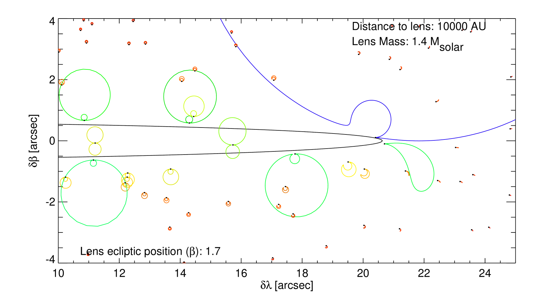
Figure 1: Illustration of the effects of a nearby lens on background sources as the lens sweeps through its parallactic ellipse (black solid line). The unlensed positions of the sources, assumed to be fixed and with no parallax, are marked with small squares. The proper motion of the lens is suppressed for illustration. Colors in the deflection tracks indicate the relative amount of the maximum deflection (longer wavelengths correspond to less departure from the unlensed position). This realization assumes a $M_{\rm X}$ = 1.4 $M_{\odot}$ NS at a low ecliptic latitude ($b=1.7^{\circ}$) with a heliocentric distance $d_{\rm X}$ = 10000 AU; the actual density of stars to the sensitivity limit of Gaia is typically lower than shown here. For other configurations of the lens, the ordinate scales as $10000$ AU/$d_{\rm X}$ and the abscissa scales as $\sin(b/1.7^{\circ})/0.0297\times(10000$ AU/$d_{\rm X})$. The normalization of the deflection angles scales as $M_{\rm X}/1.4M_{\odot}$, and, for the other Solar System deflector objects of interest, would be several orders of magnitude smaller than shown here.

The deflection tracks of background stars that are astrometrically microlensed by the motion of lens parallax (hereafter “induced parallax”) can exhibit a variety of shapes depending on the angular position with respect to the parallactic ellipse of the lens. Figure 1 shows a realization of several tracks around a neutron star at 10,000 AU. For sources at large impact parameter to the lens, the apparent positions over the year trace out a curved path along a distortion angle approximately parallel with the direction of motion of the lens at the minimum impact of the source along the parallactic ellipse. Near the position of maximal parallactic position of the lens, these curves resemble “tear drop” shapes. For impacts comparable to the semi-minor axis of the parallactic ellipse ($\Pi_{X}\sin\beta$), the deflection tracks take the appearance of “crescent” shapes or a “circle-within-circle”. This is due to comparable deflection during the nearest impact and the distant opposite-side impact months later; these such types of deflection paths are obviously more common at smaller $|\beta|$. Sources interior to the parallactic ellipse are deflected near maximally twice a year, resulting in shapes resembling a “figure eight”.

Although we call the deflection tracks due to parallactic motion of the lens “induced parallax,” the deflection tracks generally do not resemble the traditional parallactic ellipse. First, the eccentricity of the tracks does not generally scale with $\cos b$. Second, the direction of motion along the tracks is retrograde with respect to the parallactic motion of the lens. Moreover, unlike traditional parallax (where the date of maximum departure is fixed by the ecliptic azimuth), the time of maximum departure from the unlensed positions depends only on the time of minimum impact of the source to the lens. In these ways, the source parallactic motion may be distinguished from the effects due to induced parallax in principle. However, in practice the presence of intrinsic source proper motion and parallax, which are typically much larger than the signals we are concerned with here, as well as poor sampling and signal-to-noise ratio, may cause considerable degradation of the detectability. We consider these issues in more detail below.

3 Estimating the Lens Mass-Distance Sensitivity of an Astrometric Survey

Figure 1 shows a rather dramatic effect of a nearby neutron star upon a background field, with deflections of many background sources more than arcseconds from unlensed positions. Since the magnitude of the deflection tracks scales as the mass of the lens, all-sky astrometric missions could, in principle, probe to masses significantly smaller than $M_{\odot}$. We now quantify what mass/distance configurations would give rise to a detectable signal in the presence of astrometric uncertainty and a finite number of position samples of the background sources. Though the deflection of a single background source may not be detectable, clearly neighboring sources will exhibit similar, correlated deflection; therefore, the presence of a nearby massive lens can be inferred at a statistically significant level by aggregating a collection of statistically insignificant deflections.

Consider a massive body in solar orbit with mass $M_{X}$ and heliocentric distance $D_{X}$. This body will have a parallax $\Pi_{X}={\rm AU}/D_{X}$, and a proper motion $\mu_{X}=v_{X}/D_{X}$, where $v_{X}$ is its transverse velocity. If we assume that the body is in a circular orbit, and that $D_{X}\gg{\rm AU}$ (so that projection effects are small), then $v_{X}=v_{\oplus}\Pi_{X}^{1/2}$.

Now consider that the body is moving in front of a background screen of source stars with surface density $\Sigma_{*}$, and that series of $N$ astrometric measurements of these stars are taken at times $t_{j}$. At each time $t_{j}$, we can compute the deflection due to the lens $\Delta{\bf\theta}_{k}(t_{j})=[\Delta\theta_{\lambda,k}(t_{j}),\Delta\theta_{\beta,k}(t_{j})]$, for each source $k$, using the expressions presented in §2. Assuming all the source stars have the same (one-dimensional) astrometric uncertainty $\sigma_{ast}$, we can estimate the total signal-to-noise ratio ${\rm S/N}$ with which the deflection of the massive body is detected as,

$$({\rm S/N})^{2}=\frac{1}{2\sigma_{ast}^{2}}\sum_{k}\sum_{j}(\Delta\theta_{\lambda,k}(t_{j})-\langle\Delta\theta_{\lambda,k}\rangle)^{2}+(\Delta\theta_{\beta,k}(t_{j})-\langle\Delta\theta_{\beta,k}\rangle)^{2}.$$ (5)

Here $\langle\Delta\theta_{\lambda,k}\rangle$ and $\langle\Delta\theta_{\lambda,k}\rangle$ are the average deflections, i.e. $\langle\Delta\theta_{\lambda,k}\rangle\equiv N^{-1}\sum_{j}\theta_{\lambda,j}$. These are the average positions of the source determined over the course of the Gaia mission relative to some external reference grid well away from the deflector. Adopting this ${\rm S/N}$ criterion for detection is in some sense conservative, in that it only defines the significance with which the positions of the background stars differ from the null hypothesis of no deflections. The effective ${\rm S/N}$ will likely be increased by fitting a model to the data which implicitly accounts for the shape of the deflection track, as well as the correlation between neighboring sources. We note that, using the median deflections in equation (5), rather than the mean, increases the ${\rm S/N}$ by $\sim 10\%$.

We estimate the ${\rm S/N}$ using a simple Monte Carlo. We create a random screen of stars, and simulate a series of $N$ uniformly sampled measurements. We then calculate ${\rm S/N}$ using equation (5). Under our assumptions, the ${\rm S/N}$ depends on the parameters of the lens, $M_{X},\Pi_{X},\beta,t_{0},\gamma$, as well as the properties of the source stars, $\Sigma_{*},\sigma_{ast}$. We calculate ${\rm S/N}$ for many different realizations of the positions of the background source stars, and we also vary the input parameters. We find the following approximate expression for the signal-to-noise ratio,

$${\rm S/N}\simeq\left\{\begin{array}[]{ll}\frac{10\mu{\rm as}}{\sqrt{2}\sigma_{ast}}\left(\frac{M_{X}}{M_{\oplus}}\right)\left(\frac{D_{X}}{10^{3}~{}{\rm AU}}\right)^{-1}\left(\frac{\Sigma_{*}}{10^{-3}~{}{\rm arcsec}^{-2}}\right)^{1/2}\left(\frac{N}{40}\right)^{1/2}\left(1+\sin{\beta}\right)&{\rm if}\,\,\Sigma_{*}\pi\Pi_{X}^{2}\geq 1\\ \frac{10\mu{\rm as}}{\sqrt{2}\sigma_{ast}}\left(\Sigma_{*}\pi\Pi_{X}^{2}\right)^{1/2}\left(\frac{M_{X}}{M_{\oplus}}\right)\left(\frac{D_{X}}{10^{3}~{}{\rm AU}}\right)^{-1}\left(\frac{\Sigma_{*}}{10^{-3}~{}{\rm arcsec}^{-2}}\right)^{1/2}\left(\frac{N}{40}\right)^{1/2}\left(1+\sin{\beta}\right)&{\rm if}\,\,\Sigma_{*}\pi\Pi_{X}^{2}<1\end{array}\right..$$ (6)

The two regimes in equation (6) correspond to the strong, ‘collisional’ regime where there is on average one star in the parallactic ellipse, and the weak, ‘tidal’ regime where there is typically less than one star in the ellipse. Equation 6 is generally accurate to considerably better than the variance at fixed values of the parameters due to Poisson fluctuations in the number density and location of source stars, for most parameter combinations. The ${\rm S/N}$ can vary by a large amount due to Poisson noise depending on the parameters, and especially so in the tidal regime for low $\Sigma_{*}$. Note that, as reflected in equation (6), we find that the ${\rm S/N}$ does not depend on $t_{0}$ or $\gamma$ to within the Poisson fluctuations.

3.1 Application to Gaia

In order to provide a quantitative estimate of the mass-distance sensitivity of an astrometric survey to massive objects in the outer solar system, we adopt parameters appropriate for the Gaia mission. Gaia will monitor the entire sky synoptically for five years, acquiring astrometric measurements for $O(10^{9})$ stars down to apparent magnitudes of $V\sim 20$. For bright stars $(V\leq 12)$, Gaia will have a single-measurement astrometric precision limit of $30~{}\mu{\rm as}$, whereas at $V\sim 20$, the astrometric accuracy will be $\sim 1400~{}\mu{\rm as}$. Typically, each star will have $100-200$ astrometric measurements, grouped in clusters of 2 to 5 measurements each.

To proceed with our estimate, we adopt a model of the surface density of source stars on the sky as a function of magnitude, Galactic latitude and longitude, and a model of the expected astrometric performance of Gaia. This allows us to predict the total ${\rm S/N}$ with which a object of a given mass and distance would be detected with Gaia, at a given location in the sky.

The expected performance of Gaia has and will continue to evolve, and the final mission astrometric accuracy is therefore impossible to access currently. For definiteness, we assume that the (one-dimensional) astrometric uncertainty of each measurement is given by,

$$\sigma_{1D}^{2}(V)=\left\{\begin{array}[]{ll}\sigma^{2}_{sys}&{\rm if}\qquad V\leq 12.5\\ \sigma^{2}_{s}10^{0.4(V-12.5)}+\sigma^{2}_{b}10^{0.8(V-20)}&{\rm if}\qquad V>12.5\end{array},\right.$$ (7)

with $\sigma_{sys}=\sigma_{s}=30~{}\mu{\rm as}$ and $\sigma_{b}=1000\mu{\rm as}$. This form was chosen to reproduce the astrometric accuracies from Table 1 of Belokurov & Evans (2002). Gaia will not make astrometric measurements uniformly across the sky; certain ecliptic latitudes will be sampled a larger number of times than others. We assume that the number of samples as a function of ecliptic latitude $\beta$ is given by,

$$N_{samp}=100+300\exp\left[-\left(\left|\frac{|\beta|-35^{\circ}}{10^{\circ}}\right|\right)^{1/2}\right].$$ (8)

This form was chosen to qualitatively reproduce Figure 5 of Belokurov & Evans (2002). We assume that the samples are clustered into groups of $n_{c}$ points, and so the effective number of points is $N=N_{samp}/n_{c}$, and the effective astrometric accuracy of each point is $\sigma_{ast}=\sigma_{1D}(V)/\sqrt{n_{c}}$. This assumes that the single-measurement errors can be reduced by root-$n$ averaging. This may not be the case: the measurement errors in any given cluster may be correlated, or there may exist systematic errors that are not reducible. Since it is difficult to anticipate the behavior of the astrometric errors in advance, we will adopt the assumption of root-$n$ averaging for simplicity. We adopt $n_{c}=5$ (Belokurov & Evans, 2002). For other values of $n_{c}$, the ${\rm S/N}$ for any given star, as well as the integrated ${\rm S/N}$, will scale as $\sqrt{n_{c}/5}$.

We determine the surface density of source stars as a function of position and magnitude using a simple model for the Galaxy. For the density distribution of sources, we adopt the double-exponential disk plus barred bulge model of Han & Gould (1995, 2003). We assume that the dust column is independent of Galactocentric radius and has an exponential distribution in height above the plane with a scale height of $120~{}{\rm pc}$. We normalize the midplane column density so that the $V$-band extinction is $A_{V}=1~{}{\rm mag}~{}(D_{s}/{\rm kpc})$, where $D_{s}$ is the distance to the source. We also will show results assuming the dust model of Belokurov & Evans (2002), which is similar to ours for $\beta\gtrsim 20^{\circ}$, but differs in detail for latitudes closer to the plane. Finally, we assume a $V$-band luminosity function that is independent position and is equal to the Bahcall-Soneira (Bahcall & Soneira, 1980) luminosity function for $M_{V}\leq 10$, and is constant for $10\leq M_{V}\leq 20$.

The surface density of stars down to $V=20$ in our model ranges from $\sim 10^{-5}~{}{\rm arcsec}^{-2}$ near the Galactic poles, to $\sim 10^{-3}~{}{\rm arcsec}^{-2}$ near the Galactic anticenter, to a maximum of $\sim 0.1~{}{\rm arcsec}^{-2}$ within a few degrees of the Galactic center. Therefore, regions of the sky near the Galactic plane and especially the Galactic center will have greater sensitivity to lower mass and/or more distant perturbers for fixed ${\rm S/N}$. The total number of stars in the sky with $10\leq V\leq 20$ in this model is $1.3\times 10^{9}$ for our standard dust extinction model, and $1.0\times 10^{9}$ for the Belokurov & Evans (2002) dust model. Thus the average surface density is $\sim 10^{-3}~{}{\rm arcsec}^{-2}$.

Figure 2 shows the distribution of ${\rm S/N}$ for an object with $M=3000M_{\oplus}\sim 10~{}M_{\rm jup}$ and $D=10^{4}~{}{\rm AU}$ located in three different locations on the sky: near the Galactic bulge, anticenter and north Galactic pole. The source densities in these three locations vary considerably, from $\Sigma_{*}\sim 10^{-2}~{}{\rm arcsec}^{-2}$ near the Galactic bulge to $10^{-5}~{}{\rm arcsec}^{-2}$ near the pole. The shape of the distribution of ${\rm S/N}$ depends on the location on the sky, through the distribution of source densities as a function of magnitude (and so astrometric accuracy). For the locations near the Galactic plane with high source densities, the distribution of ${\rm S/N}$ has a tail toward higher values, and so the total ${\rm S/N}$ is generally dominated by one or two stars. For the location near the Galactic pole, a larger number of stars contribute significantly to the total ${\rm S/N}$. The total ${\rm S/N}$ (integrated over $V$-magnitude from $V=10$ to $V=20$) for these three locations are $({\rm S/N})_{\rm tot}=94.4$ (bulge), 16.5 (anticenter), and 1.4 (pole).

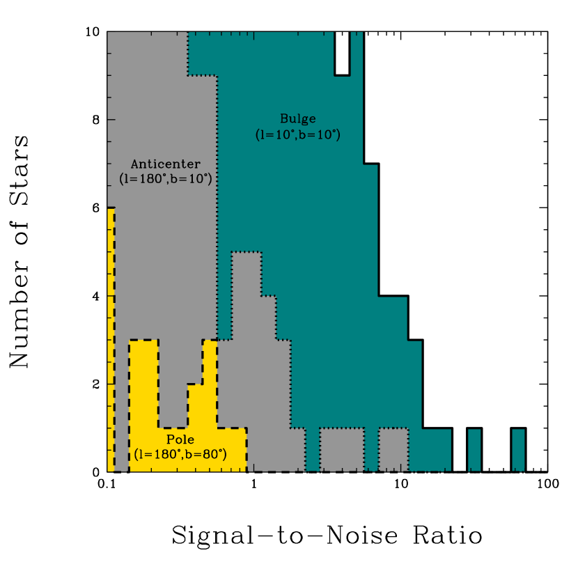
Figure 2: Distribution of signal-to-noise ratios (${\rm S/N}$) for detecting a massive object of mass $M=3000M_{\oplus}\simeq 10M_{\rm jup}$ and distance $D_{X}=10^{4}~{}{\rm AU}$ with Gaia, for various locations on the sky. The histograms show the number of stars with $10\leq V\leq 20$ as a function of the ${\rm S/N}$, for three different locations for the massive object with very different background source densities: near the Galactic bulge (solid, $l=10^{\circ},b=10^{\circ}$, $\Sigma_{*}\sim 10^{-2}$), near the Galactic anticenter (dotted, $l=180^{\circ},b=10^{\circ}$, $\Sigma_{*}\simeq 10^{-3}$), and near the north Galactic pole (dashed, $l=180^{\circ},b=80^{\circ}$, $\Sigma_{*}\simeq 10^{-5}$). For these three locations, an object with $M=3000M_{\oplus}\simeq 10M_{\rm jup}$ and $D_{X}=10^{4}~{}{\rm AU}$ would be detected at $({\rm S/N})_{\rm tot}=94.4$ (bulge), 16.5 (anticenter), and 1.4 (pole).

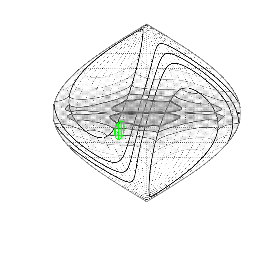
Figure 3: All sky map in Galactic coordinates of the ${\rm S/N}$ for detecting a massive object of mass $M=3000M_{\oplus}\simeq 10M_{\rm jup}$ and distance $D_{X}=10^{4}~{}{\rm AU}$ with Gaia. The dotted lines show lines of constant Galactic latitude and longitude at $15^{\circ}$ intervals. The Galactic center is located at the center of the figure. Contours of constant ${\rm S/N}$ are in grey, at levels of ${\rm S/N}=3,5,10,20,40$ (lighter to heavier). We also show lines of constant ecliptic latitude for $\beta=\pm 35^{\circ},\pm 10^{\circ},0$ (solid black lines). The oval shaded region brackets the uncertainty in the inferred position of “Planet X” from the clustering of cometary aphelion distances (Murray, 1999).

Figure 3 shows contours of constant $({\rm S/N})_{\rm tot}$ for a object with $M=3000M_{\oplus}\sim 10~{}M_{\rm jup}$ and $D=10^{4}~{}{\rm AU}$. The distribution of $({\rm S/N})_{\rm tot}$ on the sky is highly non-uniform: objects of a given $M$ and $D_{X}$ located toward certain regions of the sky will be detected with higher $({\rm S/N})_{\rm tot}$ than if they are located in other regions. The $({\rm S/N})_{\rm tot}$ is primarily driven by the surface density of stars, and therefore regions of the sky near the Galactic plane and especially the Galactic center are preferred. However, it is also the case that the number of samples $N_{samp}$ depends on ecliptic latitude, such that stars with ecliptic latitude $\sim\pm 35^{\circ}$ will have several times more astrometric measurements than stars near the ecliptic poles. Therefore locations near ecliptic latitudes of $\pm 35^{\circ}$ will also have higher $({\rm S/N})_{\rm tot}$ for fixed perturber mass and distance.

Figure 4 shows the fraction of the sky enclosed by contours of a given $({\rm S/N})_{\rm tot}$, i.e. the fraction of the sky over which an object of mass $M=3000M_{\oplus}$ and distance $D_{X}=10^{4}~{}{\rm AU}$ would be detected with ${\rm S/N}$ greater than a given value. We determine the fraction of sky above a given $({\rm S/N})_{\rm tot}$ for a range of masses and distances. Objects with mass greater than a minimum mass

$$M_{min}\simeq(290,490,750)M_{\oplus}\left\{\begin{array}[]{ll}\left(\frac{D_{X}}{10^{4}~{}{\rm AU}}\right)\left[\frac{({\rm S/N})_{\rm th}}{5}\right]&{\rm if}\,D_{X}\leq D_{b}\\ \left(\frac{D_{X}}{D_{b}}\right)\left(\frac{D_{X}}{10^{4}~{}{\rm AU}}\right)\left[\frac{({\rm S/N})_{\rm th}}{5}\right]&{\rm if}\,D_{X}>D_{b}\end{array}\right\},\,{\rm for}~{}f_{\rm sky}=(10\%,50\%,100\%).$$ (9)

can be detected with ${\rm S/N}\geq({\rm S/N})_{\rm th}$, where $f_{\rm sky}$ is the fraction of the sky. Here $D_{b}$ is the ‘break distance’, and has values of $D_{b}=(4470,1550,780){\rm AU}$ for $f_{\rm sky}=(10\%,50\%,100\%)$. These limits are shown in Figure 5.

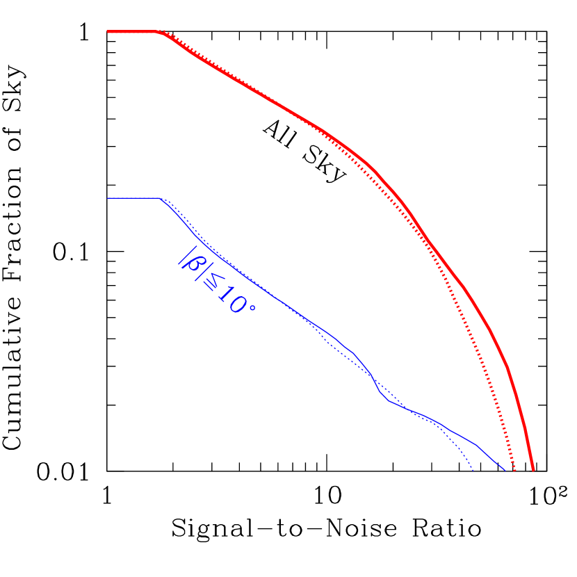
Figure 4: Fraction of the sky over which an object of mass $M=3000M_{\oplus}\simeq 10M_{\rm jup}$ and distance $D_{X}=10^{4}~{}{\rm AU}$ would be detected with ${\rm S/N}$ greater than a given value. The solid curves show the fraction assuming our fiducial model for the dust distribution, whereas the dotted lines shows the alternative model of Belokurov & Evans (2002). Upper curves are for the entire sky, the bottom curves are for ecliptic latitudes $|\beta|<10^{\circ}$.

Figure 4 also shows the fraction of the sky within $10^{\circ}$ of the ecliptic plane enclosed by contours of a given $({\rm S/N})_{\rm tot}$. Since the ecliptic plane fortuitously passes near the Galactic bulge, the slope for this curve is shallower than that for the entire sky, resulting in a relatively larger fraction of the area for which a high ${\rm S/N}$ detections are possible.

There are several obvious limitations of our calculations. One is that we have neglected the motion of background stars due to parallax. To the extent that these motions correlate with the microlensing signal, they will tend to degrade the signal-to-noise ratio, by effectively allowing one to partially ‘fit out’ the anomalous excursions. Motions of stars in binaries could also confound a clean measurement of induced parallax. Also, since we adopted the simple scaling relation in equation (6) when integrating over the magnitude distribution of source stars, we have neglected the effect of the Poisson fluctuations of the surface density and location of stars on the total signal-to-noise ratio. To provide a rough estimate of the magnitude of these effects, we have performed a few simulations where we determine the signal-to-noise ratio for stars of a given magnitude directly from the Monte Carlo simulation (which per force includes Poisson fluctuations), while explicitly fitting for the parallax of the source stars. Since these calculations are extremely time intensive, we have not performed a comprehensive exploration, but rather checked only a few cases. For these few cases, we find that fitting for the parallax of the source does indeed reduce $({\rm S/N})_{\rm tot}$, but by a relatively small factor, $\sim 10\%$. On the other hand, we find that the effect of Poisson fluctuations causes us to underestimate $({\rm S/N})_{\rm tot}$, by as much as $\sim 75\%$.

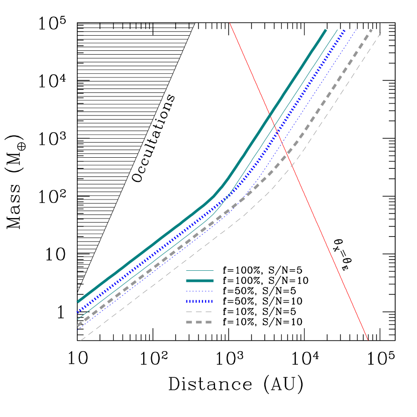
Figure 5: The lines show constraints on the mass and distance of an object that can be detected by Gaia at various ${\rm S/N}$ thresholds over various fractions of the sky. The red line shows where the angular size $\theta_{X}$ of an object with density of $1~{}{\rm g~{}cm^{-3}}$ is equal to its Einstein ring radius $\theta_{\rm E}$; objects to the left of this line have $\theta_{X}\geq\theta_{\rm E}$. Objects with parameters in the shaded region will occult at least one measurement of at least one background source, assuming a typical background source density of $2\times 10^{-3}~{}{\rm arcsec}^{-2}$.

4 Discussion and Conclusions

We have shown that a substantial, as yet unexplored, region of mass-distance parameter space of nearby massive bodies will be accessible with the current incarnation of the datastream from the Gaia experiment. We have focused on the effect of “induced parallax” caused only by the parallax of the lens as it sweeps through the parallactic ellipse. Based on our albeit simplistic simulation, the search for massive bodies in the outer Solar System by the observation of induced parallax has a reasonable chance of uncovering the proposed perturber of cometary orbits in the Oort cloud (Figs. 4 and 5). In particular, we believe that the non-detection of a massive body in the Gaia dataset using the proposed technique would relegate the proposed mass-distances of Planet X to a significantly smaller parameter space then the currently allowed space.

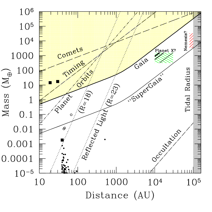
Figure 6: All-sky constraints on distant massive solar-system objects using various methods. Masses and distances to the upper left of the lines are currently excluded by these methods (‘Comets,’ ‘Planet Orbits,’ and ‘Timing’), or can be excluded in the future (‘Reflected Light,’ ‘Gaia,’ and ‘Occultation’). Limits marked ‘Comets’ and ‘Planet Orbits’ were taken from Hogg et al. (1991); the limit marked ‘Timing’ is from Zakamska & Tremaine (2005); the ‘Occultation’ limit is derived following Gaudi (2004). The line marked ‘Gaia’ shows the mass and distance of an object that can be detected by Gaia at ${\rm S/N}=5$ over 50% of the sky. The line marked “SuperGaia” shows the same limit for a hypothetical experiment with astrometric sensitivity that is two orders of magnitude better than Gaia with the same limiting magnitude. The small points show the masses and distances of known Kuiper Belt Objects (KBOs) and minor planets, where the masses were derived from their absolute magnitude assuming an albedo of $4\%$ and a density of $1~{}{\rm g~{}cm^{-3}}$. The open circles show the masses of the three recently-discovered bright KBOs 2003 EL₆₁, 2003 UB₃₁₃ and 2005 FY₉ (see Brown et al. 2005 and references therein), under the same assumptions. The large squares show the masses and distances of Uranus, Neptune, and Pluto. The shaded region at the extreme right shows the tidal radius of the solar system, $\sim 10^{5}~{}{\rm AU}$. The shaded rectangles show the range of masses and distances inferred for ‘Planet X’ and ‘Nemesis.’ Since the proposed ecliptic longitude and latitude of ‘Planet X’ (Murray, 1999) is near the Galactic plane, the limiting masses probed in that region are smaller than over the sky as a whole: the short lines passing through the shaded region labeled ‘Planet X’ show the lower limits on the mass and distance of an object that yields ${\rm S/N}=1,3,5$ (lighter to heavier) at the Murray (1999) position.

Murray (1999) made specific predictions for the current position of “Planet X” on the sky, based on the clustering of cometary aphelion distances. Since the ${\rm S/N}$ map of the sky is not uniform, it is interesting to ask with what ${\rm S/N}$ one would expect to detect “Planet X” with the allowed mass and distances, at its expected position. Figure 3 shows the positional error ellipse from Murray (1999). The expected ${\rm S/N}$ for $M_{X}=10^{3}M_{\oplus}$ and $D_{X}=10^{4}{\rm AU}$ ranges from $({\rm S/N})_{\rm tot}\simeq 3$ to $({\rm S/N})_{\rm tot}\simeq 12$. The mass/distance limit for thresholds of $({\rm S/N})_{th}=1,3$, and $5$ in this error ellipse is shown in Figure 6; roughly 25% the allowed parameter space could be excluded at $3\sigma$ with a non-detection.

Hypothesis for the mass ($\sim 0.03M_{\odot}$) and distance ($\sim 10^{5}~{}{\rm AU}$) of Nemesis will likely be difficult to test with Gaia (see Fig. 6), due primarily to the large distance and thus small size of the parallactic ellipse. However, specific predictions for the current position of Nemesis might be testable using a targeted astrometric satellite with higher astrometric precision than Gaia, such as the Space Interferometry Mission (SIM). Of course, constraints on smaller-mass objects at any distance could be obtained with with an all-sky synoptic experiment that has improved astrometric accuracy but with a similar limiting magnitude (“SuperGaia”, Fig. 6) or by probing more stars to fainter levels with Gaia-like astrometric accuracies.

Should a significant detection be made, what can be learned about the lens? In principle, the astrometric data alone provide an estimate of the mass, position, distance, and proper motion of the lens for high-${\rm S/N}$ detections of induced parallax for stars very near to the parallactic ellipse. Orbit determination will generally be difficult, unless there is a significant acceleration over the five year mission lifetime; this is only expected for relatively nearby lenses. For more modest ${\rm S/N}$ detections, or detections in the tidal regime where the source stars are quite distant from the parallactic ellipse, the information will be seriously degraded, and degeneracies between the mass, distance, and angular separation from the lens arise. In the extreme case where only one distant star is significantly perturbed, the detection may yield very little information about the lens. Exploration of the information that can be extracted from these various classes of detections is beyond the scope of this paper, but is an interesting topic for future study.

Further follow-up of potential candidates may be possible with a variety of methods. Astrometric follow-up of individual background sources may be possible with SIM with higher astrometric precision and cadence than possible with Gaia; such measurements may improve on the determination of the lens parameters. Direct detection of the reflected light from some candidates may be possible with ultra-deep imaging using very large aperture, next generation, ground-based, optical/near-infrared telescopes such as the Giant Magellan Telescope (GMT), the Thirty Meter Telescope (TMT), or the Overwhelmingly Large Telescope (OWL). Finally, the James Webb Space Telescope (JWST) should have the sensitivity to detect the thermal emission from essentially all objects detected astrometrically by Gaia.

A similar astrometric microlensing search with Gaia for massive stellar remnants in the Solar neighborhood ($d\sim 150$ pc) was proposed by Belokurov & Evans (2002) but with several important differences compared to the present work. First, we considered the detectability of an object significantly closer to Earth so that the lens parallax is $\sim 10^{5-7}$ larger than the typical source parallaxes whereas that difference is only $10^{1-2}$ for Solar neighborhood lenses. We also focused on Solar System lenses in Solar orbit where the parallax motion dominates proper motion; the motion of Solar neighborhood objects are dominated by proper motion. Both these different regimes result in significantly different microlensing tracks of a single background star (compare our Fig. 1 with Fig. 1 of Belokurov & Evans 2002). Second, we focus on detection of objects with a planet-scale mass whereas the analysis technique of Belokurov & Evans 2002 is optimized to constrain the mass function of stellar-mass objects in the Solar neighborhood (see, e.g., Fig. 3) with $M>0.1M_{\odot}$. Last, and conceptually the most distinct, we consider the detectability of a single massive object using the aggregate induced parallax signatures of thousands of stars whereas Belokurov & Evans focused on constraining the properties of a large population of faint stellar-mass objects, where the mass of each object is inferred using the astrometric microlensing “event” a single background source. Ultimately, though, both analyzes make use of the same datastream and act toward complimentary goals.

We have assumed that our lenses are point-like, and so have ignored the effects of occultation of the background sources by the lens. If the angular size of the lens $\theta_{X}$ is an appreciable fraction of its angular Einstein ring radius $\theta_{\rm E}$, then both occultation and lensing effects can potentially be important (Agol, 2002; Takahashi, 2003). In Figure 5, we show the locus of mass and distance where $\theta_{X}=\theta_{\rm E}$. Objects with $M_{X}\lesssim 10^{3}~{}M_{\oplus}$ will have angular sizes that are larger than their Einstein ring radii provided they are closer than $\sim 4000~{}{\rm AU}$; for such objects, complete occultations are possible. However, an occultation will obviously only occur if a background source happens to be located within an angular radius of the lens when a measurement is taken. This condition is met when the number of measurements satisfies $N\Sigma_{*}\pi\theta_{X}^{2}\sim 1$. Figure 5 shows the region of parameter space for which at least one measurement will be occulted by the lens, for typical background source densities of $\Sigma_{*}=2\times 10^{-3}~{}{\rm arcsec}^{-2}$. Clearly, for most lenses, occultation effects are negligible.

In our simulation, we assumed the perturber is in a circular orbit around the Sun. However, we found that our results are essentially independent of the proper motion of the lens. Furthermore, realistic motions along the line-of-sight are unlikely to alter our signal-to-noise ratio estimates substantially for the distances considered herein. Therefore, the assumption that the lens is on a circular orbit or indeed even bound to the Sun is immaterial to our conclusions.

As we have discussed, an obvious shortcoming of our estimation is that we have neglected the motion of background stars due to parallax, proper motion, and orbits. These motions will tend to degrade the signal-to-noise ratio, effectively introducing more free parameters to help explain away anomalous excursions. Still our preliminary calculations show that source parallax is not likely to degrade the ${\rm S/N}$ substantially, however these calculations were admittedly limited. We hope to perform a more comprehensive study to quantify the effect of a realistic background screen in future work.

Our simplistic simulation for S/N estimation also neglects another feature of data that could be exploited to improve the S/N. Any nearby foreground massive source will lens multiple source background stars differently in the course of a 5 year mission. Moreover, neighboring background sources will be lensed similarly. So the expectation of correlated deflection paths (which are fixed for a given lens mass, distance, and proper motion) could be used to create a “matched filter” for improving the sensitivity of detecting a nearby massive lens. Though computationally very expensive, one can envision applying such a filter to the Gaia dataset for all possible nearby lens masses at all possible distances and positions on sky to search for a signal. Aside from the need to simultaneously constrain the parallax, proper motion, and orbital parameters of all background sources, the matched filter search may also need to search for a possible changing parallax of the lens over the mission lifetime: a massive object passing nearby that is unbound to the Sun with $|v|\approx 30$ km s^-1 would travel $\approx$30 AU over 5 yr, with some of this motion in the radial direction from the Sun.

Finally, the choice of the appropriate ${\rm S/N}$ threshold for a robust detection deserves some discussion. Here one must not only consider the astrometric noise properties of the sources, but also the total number of independent trials performed in searching the data with a matched filter. This latter factor can be quite crucial in the current context, given the fact that one is performing a blind search over the entire sky with $O(10^{9})$ source stars, with many independent filters corresponding to varying lens locations, distances, masses, and proper motions.

While a high signal-to-noise ratio measurement of the entire induced parallax of single star will yield the lens mass, sky position, proper motion, and distance, the likelihood of such a special configuration is rare. Instead, each of these lens events will contribute individually to constraints on the lens properties at different times, leading to the possibility of improving the signal-to-noise ratio of the lens properties through the matched filter. Another utility of global astrometric filtering of the Gaia data is that the masses and ephemerides of known Solar System objects might be determined a priori, based solely on measurements of the astrometric microlensed background; whether the masses determined thusly will be more precise than measured by other means remains to the be seen.

References

- Agol (2002) Agol, E. 2002, ApJ, 579, 430
- Bahcall & Soneira (1980) Bahcall, J. N. & Soneira, R. M. 1980, ApJS, 44, 73
- Belokurov & Evans (2002) Belokurov, V. A. & Evans, N. W. 2002, MNRAS, 331, 649
- Brown et al. (2004) Brown, M. E., Trujillo, C., & Rabinowitz, D. 2004, ApJ, 617, 645
- Brown et al. (2005) —. 2005, IAU Circ., 8577, 1
- Byl (1983) Byl, J. 1983, Moon and Planets, 29, 121
- Davis et al. (1984) Davis, M., Hut, P., & Muller, R. A. 1984, Nature, 308, 715
- Gaudi (2004) Gaudi, B. S. 2004, ApJ, 610, 1199
- Han & Gould (1995) Han, C. & Gould, A. 1995, ApJ, 447, 53
- Han & Gould (2003) —. 2003, ApJ, 592, 172
- Hills (1981) Hills, J. G. 1981, AJ, 86, 1730
- Høg et al. (2000) Høg, E., Fabricius, C., Makarov, V. V., Urban, S., Corbin, T., Wycoff, G., Bastian, U., Schwekendiek, P., & Wicenec, A. 2000, A&A, 355, L27
- Hogg et al. (1991) Hogg, D. W., Quinlan, G. D., & Tremaine, S. 1991, AJ, 101, 2274
- Horner & Evans (2002) Horner, J. & Evans, N. W. 2002, MNRAS, 335, 641
- Hut et al. (1987) Hut, P., Alvarez, W., Elder, W. P., Kauffman, E. G., Hansen, T., Keller, G., Shoemaker, E. M., & Weissman, P. R. 1987, Nature, 329, 118
- Matese et al. (1999) Matese, J. J., Whitman, P. G., & Whitmire, D. P. 1999, Icarus, 141, 354
- Murray (1999) Murray, J. B. 1999, MNRAS, 309, 31
- Oort (1950) Oort, J. H. 1950, Bull. Astron. Inst. Netherlands, 11, 91
- Page et al. (2004) Page, D., Lattimer, J. M., Prakash, M., & Steiner, A. W. 2004, ApJS, 155, 623
- Takahashi (2003) Takahashi, R. 2003, ApJ, 595, 418
- Vandervoort & Sather (1993) Vandervoort, P. O. & Sather, E. A. 1993, Icarus, 105, 26
- Whitmire & Jackson (1984) Whitmire, D. P. & Jackson, A. A. 1984, Nature, 308, 713
- Zakamska & Tremaine (2005) Zakamska, N. L. & Tremaine, S. 2005, AJ, submitted (astro-ph/0506548)
- Zharikov et al. (2002) Zharikov, S. V., Shibanov, Y. A., Koptsevich, A. B., Kawai, N., Urata, Y., Komarova, V. N., Sokolov, V. V., Shibata, S., & Shibazaki, N. 2002, A&A, 394, 633