Millimetre continuum observations of southern massive star formation regions.
I. SIMBA observations of cold cores

Abstract

We report the results of a 1.2 mm continuum emission survey toward 131 star forming complexes suspected of undergoing massive star formation. These regions have previously been identified as harbouring a methanol maser and/or a radio continuum source (UC HII  region), whose presence is in most instances indicative of massive star formation. The 1.2 mm emission was mapped using the SIMBA instrument on the 15 m Swedish ESO Submillimetre Telescope (SEST). Emission is detected toward all of the methanol maser and UC HII  regions targeted, as well as towards 20 others lying within the fields mapped, implying that these objects are associated with cold, deeply embedded objects. Interestingly, there are also 20 methanol maser sites and 9 UC HII  regions within the fields mapped which are devoid of millimetre continuum emission.

In addition to the maser and UC HII  regions detected, we have also identified 253 other sources within the SIMBA maps. All of these (253) are new sources, detected solely from their millimetre continuum emission. These ‘mm-only’ cores are devoid of the traditional indicators of massive star formation, (i.e. methanol/OH maser, UC HII  regions, IRAS  point sources). At least 45% of these mm-only cores are also without mid-infrared MSX  emission. The ‘mm-only’ core may be an entirely new class of source that represents an earlier stage in the evolution of massive stars, prior to the onset of methanol maser emission. Or, they may harbour protoclusters which do not contain any high mass stars (i.e. below the HII  region limit).

In total, 404 sources are detected representing four classes of sources which are distinguished by the presence of the different combination of associated tracer/s. Their masses, estimated assuming a dust temperature of 20 K and adopting kinematic distances, range from 0.5 $\times 10^{1}$$M_{\odot}$  to 3.7 $\times 10^{4}$$M_{\odot}$, with an average mass for the sample of 1.5 $\times 10^{3}$$M_{\odot}$. The H₂ number density ($n_{H_{2}}$) of the source sample ranges from 1.4 $\times~{}10^{3}$ cm^-3 to 1.9 $\times~{}10^{6}$ cm^-3, with an average of 8.7 $\times~{}10^{4}$ cm^-3. The average radius of the sample is 0.5 pc. The visual extinction ranges from 10 to 500 mag with an average of 80 mag, which implies a high degree of embedding. The surface density ($\Sigma$) varies from 0.2 to 18.0 kg m^-2 with an average of 2.8 kg m^-2.

Analysis of the mm-only sources shows that they are less massive (M̄ = 0.9 $\times 10^{3}$$M_{\odot}$), and smaller (R̄ = 0.4 pc) than sources with methanol maser and/or radio continuum emission, which collectively have a mean mass of 2.5 $\times 10^{3}$$M_{\odot}$  and a mean radius of 0.7 pc.

1 Introduction

The formation of massive stars is not a well understood process neither observationally nor physically. This may be attributed to the fact that they form deeply embedded in the cores of molecular clouds, where they are optically obscured by circumstellar dust. Additionally, massive stars form on relatively short timescales, they tend to form only in clustered mode, and occur at distances greater than the nearest examples of their low mass counterparts. Consequently, the combination of these factors hinders the study of regions undergoing massive star formation, specifically the earliest processes involved in their evolution, of which there are few clear examples.

Theoretical models suggest that high mass star formation could proceed either through protostellar mergers (Bonnell et al., 2004) or through the collapse of a supersonically turbulent core (McKee & Tan, 2003). The first scenario requires dense clusters ($10^{8}$ stars pc^-3), that will trigger coalescence, whilst the second requires high accretion rates ($>10^{-3}$ $M_{\odot}$  yr^-1) that will overcome the outward radiative pressure.

To date our knowledge of the earliest stages of high-mass star formation has been limited, although recent work, as discussed in the following paragraphs, has brought new insights (c.f. Williams et al., 2004; Beuther et al., 2002; Szymczak & Kus, 2000).

Massive stars form in dense molecular clouds, and are characterised by their high luminosity ($>10^{4}$ $L_{\odot}$ ), density ($>10^{4}$ cm^-3), and strong infrared dust emission (c.f. Williams et al., 2004; Garay et al., 2003, 2004; Beuther et al., 2002). Little is known of the very earliest stages in the formation of massive stars, especially the conditions inside the early protostellar core and the putative prestellar cores. These objects are expected to be massive and cold ($\sim 20$ K) (c.f. McKee & Tan, 2003).

Methanol masers have proven particularly useful as tracers of massive star formation (e.g. Batrla et al., 1987; Caswell et al., 1995; Pestalozzi et al., 2005). Methanol masers, are occasionally associated with strong radio continuum emission (i.e. HII  regions), IRAS  far-infrared colour selected sources (e.g Wood & Churchwell (1989a) used log (F₆₀/F₁₂) $\geq$ 1.30 & log (F₂₅/F₁₂) $\geq$ 0.57), and H₂O and OH masers (Caswell et al., 1995).

Mid infrared emission from the Midcourse Space Experiment (MSX) satellite has also been used, in a similar way as IRAS, in colour selecting massive young stellar objects (MYSO). Lumsden et al. (2002) found that the MSX  colours of the youngest sources, still heavily embedded in the natal molecular clouds, are different from evolved stars which are shrouded in their own dust shells. They have developed colour-selection criteria based on MSX  colours, (F₂₁/F₈ $>$ 2) designed to deliver a list of MYSO candidates.

The coincidence of methanol masers and/or ultra compact HII  regions (UC HII) with massive star formation suggests that the two (tracers and massive stars) are inextricably linked. Consequently, maser and radio continuum emission can be used as a means of tracing regions of massive star formation (MSF). High angular resolution ($\sim 0.01^{\prime\prime}$ - $1^{\prime\prime}$) observations (Caswell, 1996; Phillips et al., 1998; Walsh et al., 1998; Minier et al., 2001) have shown that methanol masers are generally not directly associated with the UC HII  regions, but rather tend to be separated from them and possibly associated with hot molecular cores (HMCs).

Walsh et al. (1998) have reported observations where $\sim 25\%$ of UC HII  regions targeted were associated with methanol masers. In this instance, the size of the UC HII  region is generally smaller when there are masers present, suggesting such regions are possibly younger. This discovery, together with the fact that $\sim 75\%$ of the masers were not associated with UC HII  regions, led Walsh and his colleagues to propose an evolutionary sequence for massive star formation. They proposed that the methanol masers exist prior to the onset and development of the UC HII  region, the maser emission is then destroyed by an ionising region surrounding the stars, and the UC HII  region evolves following the destruction of the maser.

More recently, Walsh et al. (2003) have shown that methanol masers are associated with sub-millimetre continuum emission, and hence trace cold, deeply embedded objects.

An alternative hypothesis to explain the low correlation between UC HII  regions and methanol masers is proposed by Phillips et al. (1998). They suggest instead, that maser emission can arise from intermediate mass non-ionising stars, which yield sufficient IR photons to pump the masing transition, but insufficient UV photons to produce an UC HII  region.

In this paper, we present the results of a 1.2 millimetre continuum survey of massive star formation regions exhibiting signs of methanol maser and/or radio continuum emission. We will show that these tracers of massive star formation are in most instances associated with millimetre emission, and hence cold, deeply embedded sources. We will also present evidence of cores to which the only indicator to their existence is the millimetre continuum emission detected with the SEST. These millimetre sources (hereafter ‘mm-only cores’) are devoid of methanol maser and UC HII  emission. Other millimetre surveys have been undertaken by Beuther et al. (2002); Faúndez et al. (2004); Williams et al. (2004), and we draw attention to sources from these studies which overlap our own source list in Table 5.

The main purpose of this paper is to present the results from our study of known regions of massive star formation. In subsequent papers, we will present spectral energy distribution (SED) diagrams, which we aim to use to test current theories in the evolution of massive stars (e.g. Phillips et al., 1998; Walsh et al., 1998; Minier et al., 2005).

In section 2, we describe the observations and the data reduction procedure. The results of the SEST/SIMBA survey are discussed in $\S$3, derived physical quantities in $\S$4, and data including the sample images are presented in $\S$5. In $\S$6 we present the analysis of the data, and conclusions are given in $\S$7. The full set of images (including the ones presented in $\S 5$ as sample images) are presented in the Appendix.

2 Observations and Data Reduction

2.1 The sample

The sources chosen for this millimetre study were selected from previous studies of massive star formation regions, in particular the work of Walsh et al., as well as Thompson et al., and Minier et al., as discussed below.

The criteria for selecting the source list included:

1. sources with masers and without radio continuum emission,

2. sources with masers and with radio continuum emission,

3. radio continuum sources without methanol masers.
   

Walsh et al. (1997) undertook a study of UC HII  region candidates in search of the 6.7 GHz emission line characteristic of methanol masers. The specific UC HII  regions targeted in this survey were chosen based on their far-IR IRAS  colours according to the Wood & Churchwell (1989a) selection criteria for identifying UC HII  regions.

Thompson et al. (2004) undertook a sub-millimetre study of IRAS  point sources with associated UC HII  regions, which had previously been identified by Wood & Churchwell (1989a) and Kurtz et al. (1994).

Minier et al. (2001) observed methanol masers at very high angular resolution (10 mas), which were devoid of radio continuum emission, and were believed to be associated with high mass protostars.

The objective of our survey towards known methanol maser sites and UC HII  regions was to ascertain whether these objects are associated with millimetre continuum emission, and thus, deeply embedded objects.

2.2 Millimetre Observations

The observations were undertaken on the Swedish ESO Sub-millimetre Telescope (SEST), using the SEST IMaging Bolometer Array (SIMBA) during three separate observing periods between October 2001 and October 2002.

SIMBA is a 37-channel hexagonal bolometer array, operating at a central frequency of 250 GHz (1.2 mm), with a main beam efficiency of about 0.50 and a bandwidth of 50 GHz. SIMBA has a HPBW of $24^{\prime\prime}$ for a single element, and the separation between elements on the sky is $44^{\prime\prime}$. Observations were taken using a fixed secondary mirror in a fast mapping observing mode, with a typical scan speed of $80^{\prime\prime}s^{-1}$. The resultant pixel size of the maps, after processing is $8^{\prime\prime}$.

The initial observations were conducted during the second commissioning period of the SIMBA instrument in October 2001. 19 regions were mapped during this period. Skydips were performed every three hours in order to correct for the atmospheric opacity. Opacities stabilised around 0.35 for the first half of the night, increasing to 1.00 toward the end of the night. Maps of Jupiter were taken for calibration purposes. Typical map integration times were 15 minutes per map, mapping regions of $600^{\prime\prime}\times 384^{\prime\prime}$. The average residual noise in the maps for this period is $\sim 150$ mJy. Noise residuals in the maps may be attributed to variable sky opacities during the latter part of the observations.

The majority of the data collection took place during seven second-half nights in June 2002 (23rd–29th inclusive). During this period, observations typically spanned 8 hours each night, allowing 115 regions to be mapped. In order to accurately monitor the sky conditions, skydips were performed following every second map ($\sim 30$ minutes). Sky opacities for this period fluctuated on a nightly basis, with average values for each night listed in Table 1. No observations were taken on night three or seven due to bad weather. Maps of Uranus were taken for flux calibration purposes.

Due to a lack of suitable calibration data for the first night, the Uranus map from night four was adopted for calibration purposes, a process justified by the similar opacities for the two periods. Typical map integration times for this period were 15 minutes per source, mapping regions of $240^{\prime\prime}\times 480^{\prime\prime}$. The residual noise in the maps for this period averages around 50 mJy.

The final set of observations were taken during four nights in October 2002 (21st–24th inclusive), over a period of $\sim 5$ hours each night, mapping 38 regions in total. The sky opacity was measured regularly by taking skydips after every second observation ($\sim 30$ minutes). Sky opacities for this period fluctuated on a nightly basis, with typical values for each night listed in Table 1. Maps of Uranus were taken each night (with the exception of the first night, where Eta Car was observed) for flux calibration purposes. Due to the unsuitability of Eta Car as a flux calibrator, Uranus data from night four were used to calibrate the data from the first night (based on similar opacities for the two nights). Typical map integration times for this period were 15 minutes per source, mapping regions of $480^{\prime\prime}\times 480^{\prime\prime}$. The residual noise in the maps for this period averages around 60 mJy.

Specific calibration factors, as well as typical opacities for each night of observation are listed in Table 1 .

Table 1: Summary of the calibration factors and opacities for each night of the SEST observations. An asterisk (*) denotes calibration based on the Uranus data taken from night 4 of the same run. The dash (-) indicates that no data was taken on this occasion. Note that the opacities listed in the table are typical values for each night.

Date	Calib. Factor	Opacities
dd mm yy	$\mbox{mJy count}^{-1}$	$\tau$
	$beam^{-1}$
26th Oct 01	138.8	$\geq 0.35$
23rd Jun 02	65.9*	0.25
24th Jun 02	83.0	0.28
25th Jun 02	-	-
26th Jun 02	66.3	0.18
27th Jun 02	66.6	0.24
28th Jun 02	84.0	0.28
29th Jun 02	-	-
21st Oct 02	69.7*	0.40
22nd Oct 02	76.0	0.25
23rd Oct 02	87.7	0.28
24th Oct 02	69.4	0.30

2.3 Data Analysis

The data were reduced and analysed using the MOPSI reduction package and the procedure described in the SEST manual. In summary, the data are subject to gain elevation correction, opacity correction, baseline fitting and subtraction, despiking, deconvolution, and sky noise reduction, prior to map creation and calibration, as described in the manual.

The flux density values were obtained using the MOPSI photometry procedure described in the SEST manual. In brief, this procedure involves distinguishing the source from the background and subtracting the latter from the former, using Gaussian fitting. This technique uses polynomials to fit and subtract the baselines, and polygons to define the apertures. The MOPSI Integrate procedure, which employs the multiplication factor listed in Table 1, was used to determine the flux density of the source.

The flux density of each source was also estimated using the KARMA/KVIEW package by defining a box aperture around the source and at various points in the image considered to be the background. The flux inside of each of the apertures was then measured and the background flux was subtracted. Contour levels of 5% of the peak flux were overlaid on the sources in order to maintain source size consistency when using the box aperture.

A comparison of the flux determination via the two methods (i.e. MOPSI and KARMA) shows that there is $\leq 10\%$ difference between the two results, which arises as a consequence of the aperture definitions. Due to the greater flexibility in using the aperture applied in the MOPSI photometry procedure (i.e. polygon, which allows more accurate source definition) the fluxes determined from the MOPSI reduction procedure have been adopted as the 1.2mm flux for each of the sources, and are presented in this paper in Table 5 (see also $\S 5.2.1$ for further explanation).

The free-free emission contributing to the millimetre fluxes reported in Table 5 is expected to be negligible compared to the dust emission which dominates at 1.2 mm (F_ν $\propto$ $\nu^{-0.1}$). Assuming optically thin free-free emission for frequencies $\geq$ 8 GHz, a typical UC HII  region measured by Walsh et al. (1998) at 8  GHz to have a peak flux of 120 mJy equates to a peak flux of 85 mJy at 250 GHz, i.e. 4% of the 1.2 mm flux measured at the same position. Assuming that the 8 GHz flux measured by Walsh et al. is optically thick from a hyper compact HII  region, with the turnover frequency at 22 GHz, the 120 mJy flux measured by Walsh et al. (1998) at 8 GHz equates to 700 mJy at 1.2 mm, which would still only be significant for a small fraction of our sources. In order to be optically thick at 22 GHz, a large emission measure of 2.0 $\times 10^{9}$ cm^-6 pc is required.

Stellar winds, with $\nu^{0.6}$ (Panagia & Felli, 1975) are not expected to contribute more than $\sim 20\%$ to the flux density observed at 1.2 mm as derived from comparison of the SIMBA fluxes with typical radio fluxes measured by Walsh et al., 1998.

On at least one occasion during the June and October 2002 observations, calibration data were taken twice in a single night, in order to determine the repeatability of the data. Analysis of these Uranus maps shows less than 3% deviation in the calibration factor for the June data, and less than 1% deviation in the case of the October data. Therefore, the error resulting from measurement of the calibrator is small.

3 Results

131 known regions of massive star formation were targeted in this 1.2 mm continuum survey. The images of these regions as well as derived source properties, such as flux density and mass are presented in this paper. Of these 131 positions targeted, 69 are positions of known methanol masers, 28 have radio continuum sources, 32 are known to harbour both a methanol maser and an UC HII  region, and the remaining two are IRAS  positions. These two IRAS  positions are hereafter referred to as ‘NM-IRAS  positions’, indicating ‘no maser’ emission.

Within these 131 regions, millimetre continuum emission is detected toward a total of 404 sources, 78 of which contain methanol masers, 36 have UC HII  regions, 35 have both methanol maser and radio continuum emission, and two are the NM-IRAS  positions. The remaining 253 sources detected are ‘mm-only’ cores, to which the only indicator of their existence is the millimetre-wave continuum emission detected in this survey. As discussed below, 45% of these also have no mid-infrared emission detected by the MSX  satellite.

The mm-only cores detected by SIMBA are previously unknown and are devoid of the traditional star formation identifiers, such as methanol maser and radio continuum emission. Prior to the detection of the millimetre emission of these new cores, there was no indication (i.e. tracer) that star formation was taking place in these regions. The majority of the mm-only cores are separate from and are generally offset from the targeted tracer in the same field.

The millimetre-emitting cores are considered ‘sources’ if they are detectable at a $3\sigma$ level above the background. Many of the images presented contain multiple sources. In such fields, it is likely that all of the millimetre sources belong to the same star forming complex as the objects targeted in the fields. We have made this assumption when assigning distances (see also $\S\ref{distances}$) to the mm-only cores, based on maser velocities as presented in Table 5.

Millimetre continuum emission is detected toward all 131 of the methanol maser and UC HII  regions targeted, confirming their association with cold, deeply embedded objects. The majority of the known methanol maser and radio continuum sources are spatially encompassed within the contours of the millimetre emission, and are often directly associated with (i.e. not more than $30^{\prime\prime}$ offset from) the peak millimetre position.

In a few cases (8), the methanol maser and/or UC HII  region is quite offset from (i.e. $>30^{\prime\prime}$) the peak of the millimetre emission, yet their positions still fall within, or at the edge of, the contours of the SIMBA source. The positions of these masers, presented in Table 2, have all been determined from interferometry and are thus accurate within 1 arcsecond.

Table 2: Positions of methanol maser sites and UC HII  regions within the source contours, but offset $>30^{\prime\prime}$ from the peak millimetre continuum emission. All positions are measured by interferometry.

RA	Dec	Map	Tracer	Ref
J2000	2000	Identified
05 41 41.4	-01 53 37	G206.54-16.35	radio‡	a
05 41 45.8	-01 54 30	G206.54-16.35	radio‡	a
17 59 06.0	-24 21 16	G5.48-0.24	radio⋄	a
18 12 37.5	-18 24 08	G12.18-0.12	maser⋄	a
18 12 40.2	-18 24 47	G12.18-0.12	maser⋄	a
18 16 59.8	-16 14 50	G14.60+0.01	radio‡	a
18 34 08.1	-07 18 18	G24.47+0.49	radio‡	a
18 46 03.7	-02 41 53	G29.918-0.014	maser⋄	b

^a Positions taken from Walsh et al. (1998).
^b Positions taken from Pestalozzi et al. (2005).
^‡ Denotes sources still within contours of main source.
^⋄ Denotes sources located at the edge of the source contours.

Interestingly, the SIMBA maps also show that there are methanol maser sites and UC HII  regions devoid of millimetre continuum emission. The 20 methanol masers and 9 UC HII  regions where this occurs are listed in Table 3. The positions of the majority of these tracers ($>90\%$) have also been determined from interferometry and thus have accuracies to within 1 arcsecond. Consequently, the lack of association is not due to poor positional information. These objects are discussed further in $\S\ref{discussion}$.

Table 3: Coordinates of methanol maser sites and UC HII  regions devoid of coincident 1.2 mm continuum emission. The rms noise in the maps is typically 50-60 mJy for all sources, except for the map of G270.25+0.84 which has a rms noise value of 150 mJy. All positions have been measured from interferometry, except those sources otherwise indicated.

RA	Dec	Map	Tracer	Ref
J2000	2000	Identified
05 51 06.0	+25 45 45	G183.34+0.59	maser	c
06 08 36.1	+21 30 28	G189.03+0.76	maser	c
06 09 13.8	+21 53 13	G188.79+1.02	radio	a
09 16 41.4	-47 55 46	G270.25+0.84	maser	c
09 16 51.9	-47 54 33	G270.25+0.84	radio	b
13 14 07.0	-62 45 50	G305.55+0.01	radio	b
13 21 27.6	-63 00 48	G306.33-0.30	maser	c
16 10 25.8	-51 55 04	G330.95-0.18	radio	b
18 00 50.9	-23 21 29	G6.53-0.10	maser	b
18 00 54.1	-23 17 02	G6.53-0.10	maser$\dagger$	c
18 03 34.7	-24 24 10	G5.97-1.17	radio	b
18 03 52.4	-24 23 48	G5.97-1.17	radio	b
18 05 18.2	-19 51 15	G10.10+0.73	maser⋆	c
18 10 09.9	-19 53 22	G10.62-0.33	maser	c
18 11 48.8	-18 33 43	G12.02-0.03	radio†	b
18 12 41.0	-18 26 22	G12.18-0.12	maser	b
18 13 43.4	-17 58 06	G12.68-0.18	maser	c
18 27 13.5	-11 53 16	G19.61+0.10	maser	b
18 34 44.9	-08 31 07	G23.43-0.18	radio	b
18 36 24.0	-07 04 27	G24.84+0.08	maser	c
18 45 44.2	-02 39 04	G29.918-0.014	maser	c
18 46 09.9	-02 36 31	G29.918-0.014	maser	c
18 47 23.8	-01 42 39	G30.89+0.16	maser⋆	c
18 47 29.9	-01 54 39	G30.70-region	maser	c
18 47 37.5	-02 08 46	G30.59-0.04	maser	c
18 51 58.9	+00 07 27	G33.13 -0.09	maser	c
18 54 04.2	+02 01 36	G35.02+0.35	radio	a
19 00 14.4	+04 02 35	G37.55-0.11	maser	b
19 23 53.6	+14 34 54	G49.49-0.38	maser†	c

^a Positions taken from Kurtz et al. (1994).
^b Positions taken from Walsh et al. (1998).
^c Positions taken from Pestalozzi et al. (2005).
^† Tracer located near edge of map.
^⋆ Denotes positions determined from single dish measurements.

Examination of the SIMBA sources for mid-infrared MSX  emission reveals that 72 sources are entirely without mid-IR emission at all wavelengths (8$\mu$m, 12$\mu$m, 14$\mu$m, and 21$\mu$m); 41 are mid-IR dark clouds; and another 11 are potential mid-IR dark clouds, that is, they are sources devoid of emission, but it is unclear whether the lack of emission is due to absorption as is the case with the dark clouds, or simply a lack of emission. These associations are given in Table 5. Due to an excess of mid-IR emission in the fields examined, it is often not possible to distinguish individual associations due to confusion. Therefore the absence of an MSX  association in Table 5 does not indicate a positive mid-IR identification. Consequently, the $\sim 30\%$ of SIMBA sources which we report as having no mid infrared emission is a lower limit to the actual percentage. For these sources, the only indicator that star formation may be occurring is the millimetre continuum data detected in this survey.

The SIMBA maps also reveal two types of source located at the edge of the fields. For those sources where the emission extends off the edge of the map, the flux density is not calculated due to ambiguity in source sizes. Often the peak emission can not be reported for these sources, which are denoted by a $\beta$ in column 6 of Table 5. Sources denoted by a $\gamma$ are sources which are situated close to the edge of the map, but far enough away such that we can be reasonably confident in estimating a source size and hence a flux. However due to incomplete mapping, it is possible that the size of these sources, and hence their flux has been underestimated. Therefore the flux reported for sources denoted by a $\gamma$ is likely a lower limit.

In the case of the two NM-IRAS  positions targeted, no millimetre emission was detected at the targeted IRAS  position. These sources (G305.533+0.360 and G305.952+0.555), however, have many other millimetre sources in the SIMBA fields. We attribute these two ‘non-detections’ to the low spatial resolution offered by IRAS  in pin-pointing the peak emission of the central core.

A small selection of the images taken with the SIMBA instrument are presented in $\S 5$, Figure 1, and all of the images are presented in the Appendix. Source names are derived from their Galactic coordinates. The coordinates listed in Table 5, correspond to the position of the peak millimetre emission for each source.

4 Derivation of Physical Parameters

4.1 Mass

Assuming that the 1.2mm continuum emission detected toward these regions of massive star formation is from optically thin dust, the gas mass can be estimated using the following equation:

$$M_{gas}=\frac{S_{\nu}d^{2}}{{\kappa_{d}}B_{\nu}(T_{dust})R_{d}},$$ (1)

where $S_{\nu}$ is the 1.2mm continuum integrated flux, $d$ is the distance to the source, ${\kappa}_{d}$ is the mass absorption coefficient per unit mass of dust, $B_{\nu}$ is the Planck function for a blackbody of temperature $T_{dust}$, and $R_{d}$ is the dust to gas mass ratio.

While values of ${\kappa}_{d}$ and $R_{d}$ may vary between sources, we adopt a value of 0.1 m² kg^-1 for the mass absorption coefficient ($\kappa_{d}$) as per the opacity models of Ossenkopf & Henning (1994) (c.f. Minier et al., 2005). This gives mass estimates four times smaller than those derived using the opacity models of Hildebrand (1983). We assume a dust to gas ratio ($R_{d}$) of 1:100 (i.e. 1%). $B_{\nu}(T_{dust})$ has been evaluated for a dust temperature of 20 K (see $\S\ref{temperature}$).

The masses determined from equation 1 are listed in column 10 of Table 5. A histogram of the distribution of masses is included in Fig. 3, with a cumulative distribution shown in Fig. 4.

4.2 Temperature

The derivation of the mass of a source depends on temperature as per equation 1. Assuming that these sources are cold cores, as indicated by the presence (or lack-there-of in the instance of the mm-only cores) of methanol maser or radio continuum emission, we have assumed a temperature of 20 K for the purposes of mass derivation, which is consistent with temperatures reported in the literature. Faúndez et al. (2004) found that 1.2 mm cores associated with IRAS  sources have typical dust temperatures of 32 K, while Garay et al. (2004) found that 1.2 mm massive dust cores without emission at far infrared wavelengths have temperatures of 17 K. Minier et al. (2005) derive core temperatures $<50$ K and as low as 16 K for sources with no mid-IR emission, and Motte et al. (2003) adopt temperatures of 20-30 K for their sample of sub-millimetre cores.

We refrain from categorising the sources based on the presence of their tracer, and thus do not apply different temperatures to those cores suspected of being at different stages of evolution. We aim to constrain the temperature of each of the individual cores in forthcoming papers by compiling spectral energy distributions (SEDs). The aim of this paper is to present the images and the mass estimates for each millimetre core of the SIMBA survey.

In assuming a temperature, there is an additional uncertainty in the final mass estimate derived. We present in Table 4, the scaling factor for deriving the mass for different temperatures, from the value determined for a temperature of 20 K. For example, if the temperature were 40 K instead of 20 K, then the mass that we report will be 2.3 times larger than the actual value.

Table 4: Scaling factor for mass estimates using different temperatures to the 20 K taken here. For other temperatures, divide the value reported in Table 5 by the scaling factor in this table.

Temp.	Scaling
(K)	Factor
10	0.4
20	1.0
30	1.7
40	2.3
50	3.0
60	3.7
70	4.4

4.3 Distances

The distance for each of the methanol masers and UC HII  regions targeted in this survey is taken from the literature, and listed in column 9 of Table 5, together with the literature reference.

For the mm-only cores, we have assumed that they are at the same distance as the targeted source in the field, as indicated in column 5 of Table 5. According to Blitz (1993) the mean diameter of a giant molecular cloud (GMC) is 45 pc in diameter. Projecting the SIMBA maps on the sky, gives a spatial size of 0.4 $\times$ 0.7 pc and 20 $\times$ 40 pc for the distance extremes of 0.3 and 16.7 kpc respectively for a map size of $240^{\prime\prime}\times 480^{\prime\prime}$. Therefore all of the cores in a single map are likely to be located within the same GMC and hence we can make the assumption that the mm-only cores lie at the same heliocentric distance as the maser and/or the UC HII  region cores within the same fields.

Many of the sources have a near-far distance ambiguity. 195 sources have a clear kinematic distance, whilst for 197, the near-far distance ambiguity exists. The two NM-IRAS  positions targeted have no distance estimate. The near and far distances are listed in column 9 of Table 5, with the near distances preceding the far and separated by a ‘/’. For 12 sources in total, there is no known distance, which is indicated by the ‘Ind’ (Indeterminate) in the same column.

For analytical purposes, we have assumed the near distance for the 197 sources with a distance ambiguity (c.f. Williams et al., 2004). We do not expect the results and conclusions to be significantly affected by this assumption. As confirmation, we also analyse the sources with no distance ambiguity separately and present the results (c.f. $\S\ref{histograms}$).

G10.62-0.33 is reported by Walsh et al. (1997) to have a kinematic distance of 21.6 kpc, which has likely been overestimated. Due to the uncertainty in this distance estimate, and the close proximity of this source to G10.62-0.38 (c.f. Fig. A1, map: G10.62-0.33), we have adopted the distance of the latter to the former and its mm-only companion. According to Walsh et al. (2003) G10.62-0.38 has a kinematic distance of 6 kpc.

4.4 Source Size and H₂ Number Density ($n_{H_{2}}$)

The spatial size (FWHM) of each of the sources listed in Table 5, was determined using the Graphical Astronomy and Image Analysis Tool (GAIA). GAIA determines the FWHM (size) of the source in arcseconds, which can then be transformed into parsecs (pc) when the distance is known. Column 8 of Table 5, lists the FWHM of the sources in arcseconds, and column 4 of Table 12, lists the radius of each source in parsecs.

The H₂ number density ($n_{H_{2}}$) of each source was derived from its mass and volume estimates, assuming a spherical geometry and a mean mass per particle of $\mu~{}=~{}2.29~{}m_{H}$, which accounts for a 10% contribution of Helium (c.f. Faúndez et al., 2004). Using the parameters determined in Tables 5 and 12 (i.e. mass, radius and $n_{H_{2}}$), it is possible to determine the column density ($N_{H_{2}}$) and the surface density ($\Sigma$) of the sources in our sample. The visual extinction ($A_{v}$) of the sources can also be estimated from the column density ($N_{H_{2}}$), where, $A_{v}=N_{\rm H_{2}}/0.94\times 10^{21}$ mag (Frerking et al., 1982). The parameters of $N_{H_{2}}$, $\Sigma$ and $A_{v}$ for each of the individual sources in the sample, have not been included here, however, average values of $\Sigma$ and $A_{v}$ are reported in $\S\ref{discussion}$.

The H₂ number density of each source is listed in column 5 of Table 12. For all sources with a reported distance ambiguity in the literature, the H₂ number density ($n_{H_{2}}$) for both the near and far distances are reported, with the near preceding the far, and separated by a ‘/’. Histogram plots of the H₂ number density are given in Fig. 3, with cumulative distributions given in Fig. 4.

4.5 G10.10+0.73: an exception

G10.10+0.73 has an associated radio continuum source with a methanol maser source offset ($\sim 80^{\prime\prime}$) from it. Millimetre continuum emission is detected toward the radio continuum source, but not toward the methanol maser.

Interestingly, this maser source is also the only maser source toward which Walsh et al. (2003) did not detect submillimetre continuum emission in their SCUBA survey of methanol masers. Taking the far distance of 16.3 kpc and the 3$\sigma$ sensitivity limit of 150 mJy yields an upper limit for the mass of any continuum source at 600 $M_{\odot}$.

However the radio continuum source is associated with a planetary nebula, which would suggest that G10.10+0.73 is located at the near distance (0.3 kpc), rather than the far.

Given the Galactic latitude of G10.10+0.73, if it were located at the far distance of 16.3 kpc, then it would lie $\sim$ 200 pc above the Galactic plane. The probability of a massive star forming region existing this far above the Galactic plane seems small (Reed, 2000). Taking the near distance for the maser source, however, in accordance with this argument yields a mass of 0.2$M_{\odot}$  at a 3$\sigma$ sensitivity limit of 150 mJy at 1.2 mm. With an upper limit of 0.2$M_{\odot}$, it is unlikely that any star will form let alone develop a maser source. This therefore contradicts the previous argument and suggests that the maser source is more likely located at the far distance.

Due to the uncertainty in assigning a distance to this source, we exclude it from the following analysis.

5 Presentation of the Data

5.1 Sample Images

Each of the sources detected in this survey, has been visually classified according to its morphology. The classification scheme used is as follows:

An ‘S’ denotes singular sources. A ‘D’ indicates a single millimetre source at a contour level of 10% of the peak emission of the SIMBA map, within which there is a double core, each with their own peak of emission. An ‘A’ is assigned to those cores quite clearly differentiated as separate millimetre sources at a contour level of 10%, which are arranged spatially adjacent to each other in the SIMBA maps. Double cores differ from adjacent cores in that the emission is continuous between cores at a contour level of 10% of the peak emission, whilst for adjacent cores, there is no continuous emission between cores, indicating that they are separate cores. ‘L’ indicates those sources arranged spatially in a linear association, while ‘I’ represents those sources closely associated, and spatially arranged in an irregular arrangement. A ‘U’ is assigned to those sources whose morphology is unknown, which is usually given to those sources coincident with the edge of the map.

The sources have been further categorised according to the strength of the clustering of the core. This classification was made according to visual analysis of each of the regions, based on their angular separations. Each source has been assigned either an ‘L’, an ‘M’, or a ‘T’, indicating a low, medium or tight clustering association respectively. A low clustering association has been assigned to sources that appear in the same map, but which are distributed over a wider field than the medium and tight counterparts.

Figure 1 presents a small selection of images from this survey, chosen to highlight each of the morphological and clustering classes mentioned above. These assignments are also listed in Table 12.

Also of interest in these images presented in Fig. 1, is the indication of the source tracer. The methanol maser is depicted as a ‘plus’ symbol, while the radio continuum source is indicated by a ‘box’.

All of the images from the SIMBA survey, including those in this sample set, can be found in the Appendix. Those sources found near the centre of the frame provided the tracer used to target the position of each field.

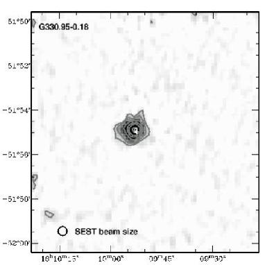
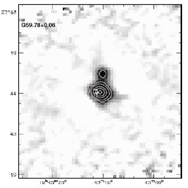
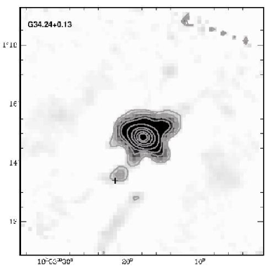
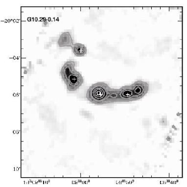
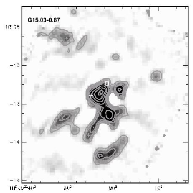
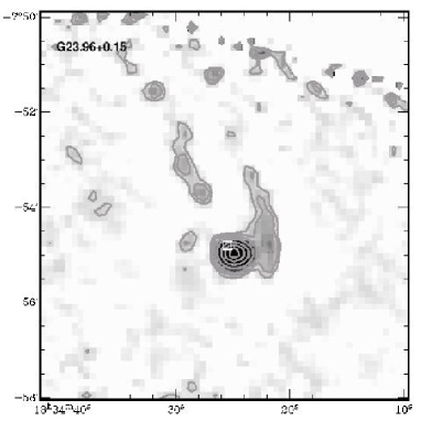
Figure 1: Sample Images from the SIMBA survey. The grey contours represent the strength of the 1.2mm continuum emission, with levels set at 10, 30, 50, 70, 90% of the peak flux. The ‘plus’ symbol represents the position of a methanol maser source, and the ‘box’ a radio continuum source (UC HII  region), which were the objects targeted in this survey. Top Left: G330.95-0.18, a singular source with the beam size of SEST indicated on the image. Top Right: G59.78+0.06 with a double core belonging to the double morphology class. Middle Left: G34.24+0.13 is representative of adjacent sources. Middle Right: G10.29-0.14, a linearly aligned region. Bottom Left: G15.03-0.67 is an example of an irregularly distributed, tightly clustered region. Bottom Right: G23.96+0.15 is an irregularly arranged region with a low degree of clustering. The entire image set from this survey can be found in the Appendix.

5.2 Physical Parameters of the Star Forming Regions

5.2.1 Main Parameters

We present the results of this survey in Table 5. The table lists all of the sources in right ascension order (RA). Columns 1 and 2 give the coordinates of the source in right ascension and declination, using J2000 epoch. Column 3 lists the source name in G-name nomenclature, derived from the Galactic coordinates of each object. Galactic names to two (or less) decimal places are consistent with those reported by Walsh et al.; Thompson et al.; Minier et al. from which they were targeted. Source names given to three decimal places, denote those sources identified in this survey, with the extended Galactic names intended to distinguish closely associated sources. Column 4 indicates the identifier of the source, where ‘$m$’, ‘$r$’, & ‘$mm$’ represent the presence of a maser, a radio continuum source, or a ‘mm-only’ source, respectively. The two NM-IRAS  sources are identified with ‘IRAS’ in the same column. Column 5 lists the millimetre map in which the source was identified (for the ‘mm-only’ sources only). Columns 6 and 7 give the integrated flux (Jy) and the peak flux ($\mbox{Jy beam}^{-1}$) for each source respectively. Column 8 gives the FWHM of each of the sources in arcseconds. Column 9 lists the distance to the source in kpc, and column 10 lists the mass of the source estimated from equation 1. For those sources for which a distance ambiguity exists, the near distance precedes the far distance as is the case with the mass estimates. Column 11 indicates the lack of an 8$\mu$m MSX  correlation, those sources devoid of mid infrared emission are denoted by an ‘N’, whilst those sources associated with a mid-IR dark cloud are denoted with a ‘DC’. An absence in this column does not indicate an MSX  correlation, since the infrared images are often too confused to distinguish whether a specific source has mid-IR emission or not. We have also drawn attention to sources previously studied in other sub-millimetre surveys such as Beuther et al. (2002); Williams et al. (2004); Faúndez et al. (2004) in column 3.

Table 5: Parameters for the 404 1.2mm continuum sources found in the survey.

Peak Position			Identifier		1.2mm Flux
RA	Dec	Source Name	Tracer	mm map	Integ.	Peak	FWHM	Distance	Mass	MSX
(J2000)	(J2000)	a			Jyb	Jy/bm	arcsecc	kpcd	$M_{\odot}$	corre
(1)	(2)	(3)	(4)	(5)	(6)	(7)	(8)	(9)	(10)	(11)
05 41 42.7	-01 54 23	G206.535-16.356	mm	G206.54-16.35	10.0	2.3	86	0.5	4.3E+01
05 41 45.4	-01 55 51	G206.54-16.35	mr		19.2	4.5	47	0.5ϵ	8.2E+01
05 51 06.0	+25 45 46	G183.34+0.59	m		5.3	1.3	45	Indζ	Ind
06 07 47.9	-06 22 57	G213.61-12.6	mr		24.3α	11.1	77	2.1ζ	1.8E+03
06 08 34.5	+20 38 51	G189.78+0.34	m		2.8	0.1	36	1.8ζ	1.5E+02
06 08 40.1	+21 31 00	G189.03+0.76	r		6.0	1.5	59	0.7ϵ	5.7E+01
06 08 45.3	+21 31 48	G189.028+0.805	mm	G189.03+0.76	2.0	0.6	47	0.7	1.7E+01
06 09 06.5	+21 50 27	G188.79+1.02	r		1.9	0.6	40	4.1η	5.5E+02
06 12 52.9	+18 00 35	G192.581-0.042	r	G192.60-0.05	4.4	2.1	42	2.6	5.0E+02
06 12 54.0	+17 59 23	G192.60-0.05	m		4.0	2.6	35	2.6ξ	4.6E+02
06 12 54.0	+17 59 47	G192.594-0.045	mm	G192.60-0.05	2.7	1.2	18	2.6	3.1E+02
08 35 31.5	-40 38 28	G259.94-0.04	m		1.9	0.8	31	Indζ	Ind
09 03 13.5	-48 55 22	G269.45-1.47	mr		1.3	0.3	55	7.9ζ	1.4E+03
09 03 32.3	-48 28 00	G269.15-1.13∗	m		5.2	2.8	31	3.6ζ	1.1E+03
09 16 41.4	-47 55 46	G270.25+0.84	m		6.8	3.6	30	2.1ζ	5.1E+02
10 23 47.0	-57 48 38	G284.271-0.391	mm	G284.35-0.42	0.4	0.1	20	4.9	1.6E+02
10 24 03.0	-57 47 58	G284.295-0.362	mm	G284.35-0.42	-β	-	-	4.9	Ind
10 24 04.0	-57 49 02	G284.307-0.376	mm	G284.35-0.42	0.6	0.2	46	4.9	2.5E+02
10 24 06.0	-57 52 06	G284.338-0.417	mm	G284.35-0.42	0.1	0.1	15	4.9	5.7E+01
10 24 10.0	-57 52 39	G284.35-0.42	m		1.3	0.5	24	4.9ζ	5.2E+02
10 24 12.0	-57 51 42	G284.345-0.404	mm	G284.35-0.42	1.4	0.4	24	4.9	5.6E+02
10 24 14.0	-57 50 46	G284.341-0.389	mm	G284.35-0.42	2.5	0.6	58	4.9	1.0E+03
10 24 15.0	-57 49 10	G284.328-0.365	mm	G284.35-0.42	0.2	0.2	14	4.9	9.0E+01
10 24 18.0	-57 54 46	G284.384-0.441	mm	G284.35-0.42	0.2	0.1	23	4.9	7.4E+01	N
10 24 21.0	-57 49 42	G284.344-0.366	mm	G284.35-0.42	1.9	0.4	24	4.9	7.9E+02
10 24 27.0	-57 49 18	G284.352-0.353	mm	G284.35-0.42	2.9γ	0.7	48	4.9	1.2E+03
10 48 05.2	-58 26 40	G287.37+0.65	m		0.8	0.4	30	5ζ	3.3E+02
10 57 33.0	-62 58 54	G290.40-2.91	m		1.5	0.6	34	3ζ	2.3E+02
11 11 33.9	-61 21 22	G291.256-0.769	mm	G291.27-0.70	2.9	0.9	42	3.1	4.7E+02	N
11 11 38.3	-61 19 54	G291.256-0.743	mm	G291.27-0.70	5.0	1.2	51	3.1	8.1E+02	DC
11 11 54.8	-61 18 26	G291.27-0.70	mr		63.0	15.5	122	3.1ζ	1.0E+04
11 12 00.6	-61 18 34	G291.288-0.706	mm	G291.27-0.70	1.2	0.7	40	3.1	1.9E+02
11 12 09.4	-61 18 10	G291.302-0.693	mm	G291.27-0.70	2.4	0.6	41	3.1	3.9E+02
11 12 15.0	-61 17 38	G291.309-0.681	mm	G291.27-0.70	6.8	1.4	61	3.1	1.1E+03	DC
11 12 16.1	-58 46 19	G290.37+1.66	m		1.5α	0.4	34	3ζ	2.3E+02
11 14 54.5	-61 13 32	G291.587-0.499	mm	G291.59-0.4	6.1	3.1	74	7.5	5.8E+03
11 14 57.8	-61 11 40	G291.576-0.468	mm	G291.59-0.4	1.8	0.7	40	7.5	1.7E+03
11 14 58.9	-61 10 36	G291.572-0.450	mm	G291.59-0.4	0.3	0.2	20	7.5	3.3E+02	N
11 15 01.1	-61 15 56	G291.608-0.532	mm	G291.59-0.4	4.1	1.2	60	7.5	3.9E+03
11 15 02.2	-61 13 40	G291.597-0.496	mm	G291.59-0.4	3.0	1.7	71	7.5	2.8E+03
11 15 06.4	-61 09 38	G291.58-0.53	m		7.5	2.3	38	7.5ζ	7.2E+03	N
11 15 08.9	-61 17 08	G291.630-0.545	mm	G291.59-0.4	11.9	2.0	82	7.5	1.1E+04
11 15 19.9	-61 11 08	G291.614-0.443	mm	G291.59-0.4	0.4	0.1	10	7.5	3.4E+02
11 32 01.4	-62 13 18	G293.824-0.762	mm	G293.82-0.74	0.5	0.2	23	10.6	9.4E+02
11 32 06.1	-62 12 22	G293.82-0.74	mr		1.8	0.8	27	10.6ζ	3.5E+03
11 32 32.4	-62 15 42	G293.892-0.782	mm	G293.82-0.74	0.2	0.1	13	10.6	3.8E+02
11 32 42.0	-62 22 35	G293.95-0.8	mr		1.2	0.6	30	11ζ	2.4E+03
11 32 42.0	-62 21 55	G293.942-0.876	mm	G293.95-0.8	1.2	0.5	29	11	2.4E+03
11 32 55.8	-62 26 11	G293.989-0.936	mm	G293.95-0.8	1.2	0.5	34	11	2.5E+03
11 35 31.0	-63 14 36	G294.52-1.60∗	m		2.2	1.0	30	1/6.1ζ	3.7E+01 / 1.4E+03
11 38 57.1	-63 28 46	G294.945-1.737	mm	G294.97-1.7	0.3	0.2	29	1.3/5.8	8.4E+00 / 1.7E+02
11 39 09.0	-63 28 38	G294.97-1.7	r		4.7	1.2	49	1.3/5.8ζ	1.4E+02 / 2.7E+03
11 39 22.1	-63 28 30	G294.989-1.720	m	G294.97-1.7	1.6	0.8	30	1.3/5.8	4.7E+01 / 9.4E+02
12 11 45.4	-61 45 42	G298.26+0.7	m		1.5	0.6	36	4ζ	4.1E+02
12 17 18.6	-62 28 40	G299.02+0.1	m		0.9	0.4	37	10ζ	1.4E+03
12 17 30.2	-62 29 04	G299.024+0.130	mm	G299.02+0.1	0.3	0.2	24	10	4.6E+02
12 29 37.3	-62 57 23	G300.455-0.190	mm	G300.51-0.1	0.4	0.2	35	9.4	5.4E+02
12 30 02.0	-62 56 35	G300.51-0.1	m		1.9	0.9	29	9.4ζ	2.8E+03
12 35 29.1	-63 01 32	G301.14-0.2	mr		16.1	6.4	70	4.4ζ	5.3E+03
12 43 32.1	-62 55 06	G302.03-0.06	mr		2.6	0.9	35	4.5ζ	8.8E+02
13 08 13.5	-62 10 20	G304.890+0.636	mm	G305.952+0.555	-β	-	-	Ind	Ind	N

Table 6: continued

Peak Position			Identifier		1.2mm Flux
RA	Dec	Source Name	Tracer	mm map	Integ.	Peak	FWHM	Distance	Mass	MSX
(J2000)	(J2000)	a			Jyb	Jy/bm	arcsecc	kpcd	$M_{\odot}$	corre
(1)	(2)	(3)	(4)	(5)	(6)	(7)	(8)	(9)	(10)	(11)
13 08 23.8	-62 13 56	G304.906+0.574	mm	G305.952+0.555	0.3	0.1	29	Ind	Ind	N
13 08 31.9	-62 15 48	G304.919+0.542	mm	G305.952+0.555	0.4	0.2	39	Ind	Ind
13 08 34.2	-62 15 00	G305.952+0.555	IRAS		-δ	-	-	Ind	Ind
13 08 35.4	-62 17 00	G304.952+0.522	mm	G305.952+0.555	0.6	0.2	39	Ind	Ind	DC
13 08 38.8	-62 15 32	G304.933+0.546	mm	G305.952+0.555	0.7	0.3	36	Ind	Ind
13 08 43.3	-62 15 16	G304.942+0.550	mm	G305.952+0.555	0.2	0.2	16	Ind	Ind
13 10 40.5	-62 34 53	G305.145+0.208	mm	G305.21+0.21	0.4	0.1	17	3.9/5.9	9.6E+01 / 2.2E+02
13 10 42.0	-62 43 13	G305.137+0.069	mm	G305.20+0.02	1.6	0.6	34	3/6.8	2.4E+02 / 1.2E+03	DC
13 11 08.3	-62 32 37	G305.201+0.241	mm	G305.21+0.21	0.2	0.4	8	3.9/5.9	4.1E+01 / 9.5E+01	N
13 11 09.4	-62 33 17	G305.202+0.230	mm	G305.21+0.21	1.4	0.4	38	3.9/5.9	3.7E+02 / 8.4E+02
13 11 12.3	-62 44 57	G305.20+0.02	r		6.2	1.9	71	3/6.8ζ	9.4E+02 / 4.8E+03
13 11 13.6	-62 47 29	G305.192-0.006	m	G305.20+0.02	2.3	0.8	31	3/6.8	3.5E+02 / 1.8E+03
13 11 14.1	-62 34 45	G305.21+0.21	m		10.6	3.1	87	3.9/5.9ι	2.7E+03 / 6.3E+03
13 11 15.9	-62 46 41	G305.197+0.007	mm	G305.20+0.02	2.3	0.7	42	3/6.8	3.6E+02 / 1.8E+03
13 11 17.0	-62 45 53	G305.200+0.02	m	G305.20+0.02	0.7	0.4	21	3/6.8	1.1E+02 / 5.8E+02
13 11 19.8	-62 30 29	G305.226+0.275	mm	G305.21+0.21	0.8	0.3	28	3.9/5.9	2.1E+02 / 4.7E+02	N
13 11 20.9	-62 29 48	G305.228+0.286	mm	G305.21+0.21	0.2	0.1	14	3.9/5.9	3.9E+01 / 8.9E+01	N
13 11 26.7	-62 31 16	G305.238+0.261	mm	G305.21+0.21	1.4α	0.3	47	3.9/5.9	3.6E+02 / 8.2E+02	N
13 11 30.3	-62 33 24	G305.242+0.225	mm	G305.21+0.21	0.2	0.1	14	3.9/5.9	6.2E+01 / 1.4E+02
13 11 32.5	-62 32 12	G305.248+0.245	m	G305.21+0.21	1.2	0.5	32	3.9/5.9	3.1E+02 / 7.1E+02
13 11 35.8	-62 48 16	G305.233-0.023	mm	G305.20+0.02	0.7	0.3	38	3/6.8	1.0E+02 / 5.1E+02	N
13 11 54.4	-62 47 19	G305.269-0.010	mm	G305.20+0.02	3.4γ	1.3	65	3/6.8	5.2E+02 / 2.7E+03
13 12 30.5	-62 34 43	G305.355+0.194	mm	G305.37+0.21	-α	-	-	3/6.8	Ind
13 12 31.6	-62 34 11	G305.358+0.203	mm	G305.37+0.21	17.9α	3.2	98	3/6.8	2.7E+03 / 1.4E+04
13 12 34.7	-62 35 15	G305.362+0.185	m	G305.37+0.21	3.5	2.3	56	3/6.8	5.3E+02 / 2.7E+03
13 12 35.2	-62 37 15	G305.361+0.151	m	G305.37+0.21	5.3	1.4	33	3/6.8	8.2E+02 / 4.2E+03
13 12 36.3	-62 33 39	G305.37+0.21	r		5.8	1.6	56	3/6.8ι	8.8E+02 / 4.5E+03
13 12 38.1	-62 36 42	G305.340-0.172	mm	G305.37+0.21	0.5	0.2	35	3/6.8	8.1E+01 / 4.2E+02
13 13 46.0	-62 25 37	G305.513+0.333	mm	G305.533+0.360	0.1	0.3	13	Ind	Ind	N
13 13 55.2	-62 23 53	G305.533+0.360	IRAS		-δ	-	-	Ind	Ind
13 13 58.7	-62 25 05	G305.538+0.340	mm	G305.533+0.360	1.1	0.6	41	Ind	Ind
13 14 06.1	-62 47 53	G305.519-0.040	mm	G305.55+0.01	-β	-	-	3.6/6.3	Ind
13 14 06.1	-62 46 41	G305.520-0.020	mm	G305.55+0.01	0.2	0.1	22	3.6/6.3	4.2E+01/ 1.3E+02
13 14 20.0	-62 45 13	G305.549+0.002	mm	G305.55+0.01	1.0	0.3	41	3.6/6.3	2.2E+02 / 6.8E+02
13 14 21.2	-62 44 33	G305.55+0.01	m		0.9	0.5	35	3.6/6.3ζ	2.1E+02 / 6.4E+02
13 14 22.4	-62 46 01	G305.552+0.012	mm	G305.55+0.01	2.0	0.7	61	3.6/6.3	4.5E+02 / 1.4E+03
13 14 25.8	-62 44 32	G305.561+0.012∗	r	G305.55+0.01	3.2	1.1	76	3.6/6.3	7.1E+02/ 2.2E+03
13 14 35.1	-62 43 02	G305.581+0.033	mm	G305.55+0.01	0.5α	0.1	78	3.6/6.3	1.2E+02 / 3.7E+02
13 14 49.1	-62 44 24	G305.605+0.010	mm	G305.55+0.01	0.3	0.1	35	3.6/6.3	6.6E+01 / 2.0E+02
13 16 31.5	-62 59 02	G305.776-0.251	mm	G305.81-0.25	0.4	0.2	32	3.9/6	1.1E+02/ 2.7E+02
13 16 39.6	-62 57 49	G305.81-0.25	mr		6.1	3.0	52	3.9/6ζ	1.6E+03 / 3.8E+03
13 16 58.3	-62 55 25	G305.833-0.196	mm	G305.81-0.25	0.5	0.2	34	3.9/6	1.3E+02 / 3.2E+02	N
13 21 18.2	-63 00 43	G306.33-0.3	m		0.5	0.2	32	2/8.1ζ	3.2E+01 / 5.3E+02
13 21 18.2	-63 01 07	G306.319-0.343	mm	G306.33-0.3	0.2	0.1	12	2/8.1	1.0E+01 / 1.7E+02
13 21 32.3	-62 58 26	G306.343-0.302	mm	G306.33-0.3	0.7	0.1	14	2/8.1	4.5E+01 / 7.4E+02	N
13 21 34.6	-62 59 54	G306.345-0.345	mm	G306.33-0.3	0.4	0.1	14	2/8.1	2.9E+01 / 4.8E+02
13 50 38.2	-61 34 20	G309.917+0.494	mm	G309.92+0.4	0.2	0.1	15	5.5	9.8E+01	N
13 50 41.6	-61 35 15	G309.92+0.4∗	m		5.5	2.2	64	5.5μ	2.8E+03
15 00 33.6	-58 58 05	G318.913-0.162	r	G318.92-0.68	3.5	1.6	35	2	2.4E+02
15 00 55.3	-58 58 54	G318.92-0.68	m		4.8	1.9	36	2μ	3.3E+02
15 31 41.6	-56 30 11	G323.74-0.3	m		5.9	2.6	36	3.4/10.3ι	1.2E+03 / 1.1E+04
16 09 48.8	-51 53 51	G330.95-0.18	mr		32.8	15.3	90	5.3/9.6ι	1.6E+04 / 5.2E+04
16 11 26.9	-51 41 57	G331.28-0.19∗	m		6.9	1.9	-$\ddagger$	4.7/10.1ι	2.6E+03 / 1.2E+04
16 19 30.5	-51 02 40	G332.640-0.586	mm	G332.73-0.62	0.7	0.3	16	3.3/11.8	1.3E+02 / 1.7E+03
16 19 38.1	-51 03 12	G332.648-0.606∗	m	G332.73-0.62	15.7α	1.8	134	3.3/11.8	2.9E+03 / 3.7E+04
16 19 47.4	-51 00 08	G332.701-0.587	mm	G332.73-0.62	0.8	0.3	30	3.3/11.8	1.5E+02 / 1.9E+03
16 19 48.3	-51 02 00	G332.646-0.647	mm	G332.73-0.62	2.0	0.8	30	3.3/11.8	3.7E+02 / 4.8E+03
16 19 51.7	-51 01 20	G332.695-0.609	mm	G332.73-0.62	3.9	1.3	43	3.3/11.8	7.3E+02 / 9.3E+03
16 20 02.7	-51 00 32	G332.73-0.62	m		0.6	0.3	11	3.3/11.8ζ	1.1E+02 / 1.4E+03	N
16 20 07.0	-50 56 48	G332.777-0.584	mm	G332.73-0.62	0.6	0.3	15	3.3/11.8	1.2E+02 / 1.5E+03	N
16 20 07.0	-51 00 00	G332.627-0.511	mm	G332.73-0.62	0.5	0.3	13	3.3/11.8	9.1E+01 / 1.2E+03	DC

Table 7: continued

Peak Position			Identifier		1.2mm Flux
RA	Dec	Source Name	Tracer	mm map	Integ.	Peak	FWHM	Distance	Mass	MSX
(J2000)	(J2000)	a			Jyb	Jy/bm	arcsecc	kpcd	$M_{\odot}$	corre
(1)	(2)	(3)	(4)	(5)	(6)	(7)	(8)	(9)	(10)	(11)
16 20 12.0	-50 53 20	G332.827-0.552∗	mm	G332.73-0.62	-β	-	-	3.3/11.8	Ind
16 20 15.0	-50 56 40	G332.794-0.598	mm	G332.73-0.62	0.9	0.3	25	3.3/11.8	1.7E+02 / 2.2E+03
17 45 54.3	-28 44 08	G0.204+0.051	mm	G0.21-0.00	0.6	0.3	37	8.4/8.6	7.5E+02 / 7.8E+02	DC
17 46 03.9	-28 24 58	G0.49+0.19	m		1.2	0.5	30	2.6/14.5ζ	1.4E+02 / 4.4E+03
17 46 07.1	-28 41 28	G0.266-0.034	mm	G0.21-0.00	1.0	0.4	37	8.4/8.6	1.2E+03 / 1.2E+03	DC
17 46 07.7	-28 45 20	G0.21-0.00	mr		1.2	0.4	42	8.4/8.6ζ	1.5E+03 / 1.6E+03
17 46 08.2	-28 25 23	G0.497+0.170	mm	G0.49+0.19	0.9	0.2	26	2.6/14.5	1.0E+02 / 3.2E+03
17 46 09.5	-28 43 36	G0.24+0.01	mm	G0.21-0.00	7.2	1.2	74	8.4/8.6	8.6E+03 / 9.0E+03	DC
17 46 10.1	-28 23 31	G0.527+0.181	r	G0.49+0.19	2.4	0.8	38	2.6/14.5	2.8E+02 / 8.7E+03
17 46 10.7	-28 41 36	G0.271+0.022	mm	G0.21-0.00	0.6α	0.3	31	8.4 / 8.6	6.9E+02 / 7.2E+02	DC
17 46 11.4	-28 42 40	G0.26+0.01	mm	G0.21-0.00	6.7	1.2	119	8.4/8.6	8.0E+03 / 8.4E+03	DC
17 46 52.8	-28 07 35	G0.83+0.18	m		1.2	0.5	29	4.5/12.5ζ	4.2E+02 / 3.3E+03
17 47 00.0	-28 45 20	G0.331-0.164	mm	G0.32-0.20	0.8	0.2	28	8/9	8.6E+02 / 1.1E+03
17 47 01.2	-28 45 36	G0.310-0.170	mm	G0.32-0.20	0.2	0.1	12	8/9	1.9E+02 / 2.3E+02
17 47 09.1	-28 46 16	G0.32-0.20	mr		5.9	1.2	126	8/9ζ	6.4E+03 / 8.1E+03
17 47 20.1	-28 47 04	G0.325-0.242	mm	G0.32-0.20	0.3	0.1	11	8/9	3.5E+02 / 4.4E+02	DC
17 48 31.6	-28 00 31	G1.124-0.065	mm	G1.13-0.11	0.5	0.2	28	8.5	5.9E+02
17 48 34.7	-28 00 16	G1.134-0.073	mm	G1.13-0.11	0.2	0.1	18	8.5	2.5E+02
17 48 36.4	-28 02 31	G1.105-0.098	mm	G1.14-0.12	1.8	0.4	19	8.5	2.2E+03
17 48 41.9	-28 01 44	G1.13-0.11∗	r		7.9	1.7	115	8.5η	9.7E+03
17 48 48.5	-28 01 13	G1.14-0.12	m		0.2	0.2	47	8.5ι	3.0E+02
17 50 14.5	-28 54 31	G0.55-0.85	mr		15.8	5.7	94	2χ	1.1E+03
17 50 18.8	-28 53 14	G0.549-0.868	mm	G0.55-0.85	4.0	0.2	70	2	2.7E+02
17 50 24.9	-28 50 15	G0.627-0.848	mm	G0.55-0.85	0.3	0.2	26	2	2.2E+01	N
17 50 26.7	-28 52 23	G0.600-0.871	mm	G0.55-0.85	0.8	0.3	39	2	5.7E+01	N
17 50 46.5	-26 39 45	G2.54+0.20	m		2.1	0.4	63	2.7/14.2ζ	2.6E+02 / 7.2E+03	DC
17 59 04.6	-24 20 55	G5.48-0.24	r		1.1	0.3	39	12.5ν	3.0E+03
17 59 07.5	-24 19 19	G5.504-0.246	mm	G5.48-0.24	0.7	0.1	31	12.5	1.9E+03	N
18 00 31.0	-24 03 59	G5.89-0.39	r		23.2	9.5	90	2.6ν	2.7E+03
18 00 40.9	-24 04 21	G5.90-0.42	m		8.1	2.9	62	2.7/14.2ζ	1.0E+03 / 2.8E+04
18 00 43.9	-24 04 47	G5.90-0.44	mm	G5.90-0.42	5.0	1.5	69	2.7/14.2	6.2E+02 / 1.7E+04
18 00 50.9	-23 21 29	G6.53-0.10	r		3.0	0.9	41	14ν	1.0E+04
18 00 54.1	-23 17 02	G6.60-0.08⋆	m		0.3	0.1	15	0.3/16.6ζ	5.4E-01 / 1.6E+03
18 00 59.2	-23 17 02	G6.620-0.100⋆	mm	G6.60-0.08	0.2	0.1	21	0.3/16.6	3.7E-01 / 1.1E+03	N
18 02 52.8	-21 47 54	G8.127+0.255	mm	G8.13+0.22	0.9	0.2	31	3.4	1.7E+02	N
18 02 56.2	-21 47 38	G8.138+0.246	mm	G8.13+0.22	1.9	0.5	66	3.4	3.6E+02
18 03 00.8	-21 48 10	G8.13+0.22∗	mr		8.0	2.0	69	3.4ν	1.6E+03
18 03 26.3	-24 22 29	G5.948-1.125	mm	G5.97-1.17	0.3	0.2	39	1.9	2.0E+01	N
18 03 34.5	-24 21 41	G5.975-1.146	mm	G5.97-1.17	0.5	0.2	29	1.9	2.8E+01	N
18 03 36.8	-24 22 13	G5.971-1.158	mm	G5.97-1.17	0.8	0.5	48	1.9	5.0E+01
18 03 40.9	-24 22 37	G5.97-1.17	r		9.2	2.2	88	1.9ν	5.7E+02
18 05 15.6	-19 50 55	G10.10+0.73	r		0.6	0.4	30	0.4/16.3ι	0.2E+01 / 2.9E+03
18 06 14.8	-20 31 37	G9.62+0.19∗	mr		8.5	3.3	94	2μ	5.8E+02
18 06 18.9	-21 37 21	G8.67-0.36	mr		13.9	5.0	81	4.7ν	5.2E+03
18 06 23.5	-21 36 57	G8.686-0.366	m	G8.67-0.36	3.4	1.4	55	4.7	1.3E+03	DC
18 06 24.6	-21 40 01	G8.644-0.395	mm	G8.67-0.36	0.3	0.2	26	4.7	1.1E+02	DC
18 06 26.4	-21 35 29	G8.713-0.364	mm	G8.67-0.36	0.9	0.3	66	4.7	3.2E+02	DC
18 06 28.7	-21 34 17	G8.735-0.362	mm	G8.67-0.36	1.5γ	0.3	66	4.7	5.7E+02
18 06 36.1	-21 36 01	G8.724-0.401a	mm	G8.67-0.36	0.2	0.2	21	4.7	8.3E+01	DC
18 06 36.7	-21 37 05	G8.724-0.401b	mm	G8.67-0.36	0.6	0.3	35	4.7	2.1E+02	DC
18 06 37.3	-21 36 33	G8.718-0.410	mm	G8.67-0.36	0.1	0.1	8	4.7	5.3E+01	DC
18 07 45.8	-20 19 47	G9.966-0.020	mm	G9.99-0.03	0.2	0.1	10	5.0	8.1E+01	N
18 07 50.4	-20 18 51	G9.99-0.03	m		1.2	0.6	45	5.0χ	5.2E+02	N
18 07 53.2	-20 18 19	G10.001-0.033	r	G9.99-0.03	0.4	0.2	22	5.0	1.5E+02
18 08 37.9	-19 51 41	G10.47+0.02∗	mr		24.0α	10.1	122	6/10.8ζ	1.5E+04 / 4.8E+04
18 08 44.9	-19 54 38	G10.44-0.01	m		1.6	0.6	51	5.9/10.8ζ	9.4E+02 / 3.2E+03	DC
18 08 45.9	-20 05 34	G10.287-0.110	mm	G10.32-0.15	2.8	1.0	54	1.8/15	1.6E+02 / 1.1E+04	N
18 08 49.4	-20 05 58	G10.284-0.126	m		2.6	1.1	46	1.9ν	1.6E+02
18 08 52.4	-20 05 58	G10.288-0.127	mm	G10.32-0.15	0.9	0.6	40	1.8/15	5.2E+01 / 3.6E+03
18 08 55.5	-20 05 58	G10.29-0.14	mr		7.8	2.5	73	1.9ν	4.8E+02
18 09 00.0	-20 05 34	G10.343-0.142	m	G10.32-0.15	1.7	0.9	26	1.8/15	9.6E+01 / 6.6E+03

Table 8: continued

Peak Position			Identifier		1.2mm Flux
RA	Dec	Source Name	Tracer	mm map	Integ.	Peak	FWHM	Distance	Mass	MSX
(J2000)	(J2000)	a			Jyb	Jy/bm	arcsecc	kpcd	$M_{\odot}$	corre
(1)	(2)	(3)	(4)	(5)	(6)	(7)	(8)	(9)	(10)	(11)
18 09 01.5	-20 05 08	G10.32-0.15	m		5.5	1.2	108	1.8/15ζ	3.0E+02 / 2.1E+04
18 09 03.5	-20 02 54	G10.359-0.149	mm	G10.32-0.15	1.4	0.4	47	1.8/15	8.0E+01 / 5.5E+03	N
18 09 14.2	-20 18 53	G10.146-0.314	mm	G10.15-0.34	0.5	0.2	43	6	3.0E+02
18 09 18.2	-20 16 21	G10.191-0.307	mm	G10.15-0.34	0.2	0.7	11	6	9.8E+01
18 09 18.2	-20 19 17	G10.148-0.331	mm	G10.15-0.34	-α	-	37	6	Ind
18 09 20.5	-20 15 01	G10.214-0.305	mm	G10.15-0.34	0.2	0.1	16	6	1.0E+02	DC
18 09 21.6	-20 16 21	G10.191-0.308	mm	G10.15-0.34	0.5	0.2	29	6	3.0E+02	DC
18 09 21.6	-20 19 25	G10.15-0.34	r		6.5	1.4	70	6ν	4.0E+03
18 09 25.0	-20 15 41	G10.213-0.326	mm	G10.15-0.34	3.9	1.1	62	6	2.4E+03	DC
18 09 26.2	-20 17 33	G10.188-0.344	mm	G10.15-0.34	1.0	0.4	58	6	5.9E+02	DC?
18 09 26.7	-20 21 25	G10.133-0.378	mm	G10.15-0.34	0.4	0.2	30	6	2.3E+02
18 09 26.7	-20 19 17	G10.164-0.360	mm	G10.15-0.34	7.7α	1.2	109	6	4.7E+03
18 09 28.4	-20 14 29	G10.237-0.328	mm	G10.15-0.34	0.1	0.1	15	6	7.4E+01	DC
18 09 29.6	-20 16 45	G10.206-0.350	mm	G10.15-0.34	1.0	0.6	56	6	6.4E+02	N
18 09 31.3	-20 18 29	G10.184-0.370	mm	G10.15-0.34	0.2	0.1	17	6	1.4E+02
18 09 33.5	-20 17 49	G10.198-0.372	mm	G10.15-0.34	0.3	0.2	30	6	2.0E+02	N
18 09 34.6	-20 22 21	G10.138-0.419	mm	G10.15-0.34	0.2	0.1	20	6	1.2E+02	DC
18 09 35.3	-20 21 25	G10.149-0.407	mm	G10.15-0.34	0.3	0.2	29	6	2.1E+02	N
18 09 36.4	-20 20 29	G10.165-0.403	mm	G10.15-0.34	0.4	0.2	29	6	2.1E+02	N
18 09 36.4	-20 18 29	G10.194-0.387	mm	G10.15-0.34	0.5	0.2	30	6	3.0E+02	DC
18 09 39.2	-20 19 25	G10.186-0.404	mm	G10.15-0.34	0.2γ	0.1	12	6	1.0E+02
18 10 14.5	-19 57 17	G10.575-0.347	mm	G10.62-0.33	-β	0.2	-	6.0	Ind	N
18 10 15.7	-19 54 45	G10.63-0.33B	mm	G10.62-0.33	1.4	0.5	56	6.0	8.7E+02
18 10 18.0	-19 54 05	G10.62-0.33	m		3.7	0.7	63	6.0ι	2.2E+03
18 10 19.0	-20 45 33	G9.88-0.75	r		5.5	0.9	117	3.9ϵ	1.4E+03
18 10 24.1	-20 43 09	G9.924-0.749	mm	G9.88-0.75	0.7	0.3	42	3.9	1.7E+02
18 10 29.4	-19 55 41	G10.62-0.38	mr		27.9	10.2	111	6.0ν	1.7E+04
18 10 41.1	-19 57 41	G10.620-0.441	mm	G10.62-0.33	0.4	0.2	19	6.0	2.3E+02	N
18 11 24.4	-19 32 04	G11.075-0.384	mm	G11.11-0.34	0.9	0.3	38	5.2	4.0E+02
18 11 31.8	-19 30 44	G11.11-0.34	r		3.3	0.9	91	5.2ϵ	1.5E+03
18 11 35.8	-19 30 44	G11.117-0.413	mm	G11.11-0.34	0.5	0.3	31	5.2	2.5E+02	N
18 11 51.4	-17 31 30	G12.88+0.48⋄†∗	m		6.9	2.4	87	4/12.5ζ	1.9E+03 / 1.8E+04
18 11 52.9	-18 36 03	G11.948-0.003	mm	G12.02-0.03	1.2γ	0.5	42	6.6/10	9.0E+02 / 2.1E+03
18 11 53.6	-17 30 02	G12.914+0.493†	mm	G12.88+0.48	0.7	0.4	29	4/12.5	2.0E+02 / 2.0E+03
18 12 01.9	-18 31 56	G12.02-0.03⋄	m		0.6	0.2	28	6.6/10ζ	4.1E+02 / 9.4E+02
18 12 02.1	-18 40 26	G11.902-0.100	mm	G11.93-0.14	0.2	0.1	16	4.6/12.1	6.5E+01 / 4.5E+02	N
18 12 11.1	-18 41 27	G11.903-0.140	mr	G11.93-0.14	2.2	0.7	77	4.6/12.1	7.9E+02 / 5.5E+03	N
18 12 15.6	-18 44 58	G11.861-0.183	mm	G11.93-0.14	0.1	0.1	15	4.6/12.1	4.3E+01 / 3.0E+02	N
18 12 17.3	-18 40 03	G11.93-0.14	m		0.6	0.3	31	4.6/12.1ι	2.3E+02 / 1.6E+03
18 12 19.6	-18 39 54	G11.942-0.157	mm	G11.93-0.14	0.7	0.3	34	4.6/12.1	2.3E+02 / 1.6E+03
18 12 23.5	-18 22 49	G12.200-0.003	mm	G12.20-0.09	0.7	0.5	28	14	2.4E+03
18 12 25.7	-18 39 46	G11.956-0.177	mm	G11.93-0.14	0.1	0.1	13	4.6/12.1	4.0E+01 / 2.7E+02	N
18 12 33.1	-18 30 05	G12.112-0.125	mm	G12.18-0.12	0.6	0.3	50	14	1.9E+03	N
18 12 39.2	-18 24 17	G12.20-0.09	mr		4.3	2.3	73	14ν	1.4E+04
18 12 41.6	-18 24 47	G11.942-0.256	mm	G11.99-0.27	0.6	0.3	26	5.2/11.4	2.9E+02 / 1.4E+03	N
18 12 42.7	-18 25 08	G12.18-0.12	m		0.6	0.1	42	14ν	2.1E+03
18 12 44.4	-18 24 25	G12.216-0.119	mm	G12.18-0.12	1.2	0.5	25	14	3.9E+03
18 12 51.2	-18 40 40	G11.99-0.27	m		0.3	0.2	28	5.2/11.4ζ	1.5E+02 / 7.3E+02
18 12 56.4	-18 11 04	G12.43-0.05	r		0.9	0.2	42	16.7ν	4.1E+03
18 13 54.7	-18 01 41	G12.68-0.18	m		5.6	1.3	102	4.7/11.8ζ	2.1E+03 / 1.3E+04
18 13 58.5	-18 54 21	G11.94-0.62B	mm	G11.93-0.61	4.5	1.3	65	3.6	9.8E+02	N
18 14 00.9	-18 53 27	G11.93-0.61∗	mr		5.9	2.2	67	3.6ν	1.3E+03
18 14 07.6	-18 00 37	G12.722-0.218	mm	G12.68-0.18	1.9	0.8	50	4.7/11.8	7.2E+02 / 4.5E+03
18 14 25.5	-17 53 52	G12.855-0.226	mm	G12.90-0.26	-β	-	-	3.9/12.6	Ind
18 14 28.3	-17 52 08	G12.885-0.222	mm	G12.90-0.26	0.4	0.2	18	3.9/12.6	1.0E+02 / 1.1E+03
18 14 30.0	-17 51 52	G12.892-0.226	mm	G12.90-0.26	0.3	0.2	21	3.9/12.6	6.5E+01 / 6.8E+02
18 14 34.3	-17 51 56	G12.90-0.25B	mm	G12.90-0.26	1.6	0.8	62	3.9/12.6	4.1E+02 / 4.3E+02	DC?
18 14 36.1	-17 54 56	G12.859-0.272	mm	G12.90-0.26	2.3	0.7	50	3.9/12.6	5.9E+02 / 6.2E+03
18 14 36.1	-16 45 44	G13.87+0.28	m		6.0	1.8	79	4.5η	2.1E+03
18 14 39.5	-17 52 00	G12.90-0.26∗	m		8.6	2.4	90	3.9/12.6ι	2.2E+03 / 2.3E+04
18 14 41.7	-17 54 24	G12.878-0.226	mm	G12.90-0.26	0.3	0.2	24	3.9/12.6	7.0E+01 / 7.3E+02

Table 9: continued

Peak Position			Identifier		1.2mm Flux
RA	Dec	Source Name	Tracer	mm map	Integ.	Peak	FWHM	Distance	Mass	MSX
(J2000)	(J2000)	a			Jyb	Jy/bm	arcsecc	kpcd	$M_{\odot}$	corre
(1)	(2)	(3)	(4)	(5)	(6)	(7)	(8)	(9)	(10)	(11)
18 14 42.9	-17 53 12	G12.897-0.281	mm	G12.90-0.26	0.3	0.1	12	3.9/12.6	6.7E+01 / 7.0E+02	N
18 14 44.5	-17 52 16	G12.914-0.280	mm	G12.90-0.26	0.2	0.2	14	3.9/12.6	6.2E+01 / 6.5E+02
18 14 45.7	-17 50 48	G12.938-0.272	mm	G12.90-0.26	0.2	0.1	11	3.9/12.6	5.4E+01 / 5.7E+02
18 16 22.1	-19 41 27	G11.49-1.48∗	m		4.9	1.5	97	1.1/15.6ζ	1.0E+02 / 2.0E+04
18 17 00.5	-16 14 44	G14.60+0.01	mr		2.2	0.8	78	2.8/13.7ζ	3.0E+02 / 7.2E+03
18 19 12.6	-20 47 31	G10.84-2.59	r		5.0	2.0	74	1.9ϵ	3.1E+02
18 20 10.3	-16 10 35	G15.022-0.618	mm	G15.03-0.37	1.7	0.8	30	2.4/14	1.7E+02 / 5.7E+03	DC
18 20 17.6	-16 13 55	G14.987-0.670	mm	G15.03-0.37	1.5	0.8	24	2.4/14	1.4E+02 / 4.9E+03	DC?
18 20 18.1	-16 11 15	G15.027-0.651	mm	G15.03-0.37	5.5	2.4	51	2.4/14	5.4E+02 / 1.8E+04	N
18 20 19.2	-16 09 31	G15.054-0.641	mm	G15.03-0.37	0.7	0.5	18	2.4/14	6.5E+01 / 2.2E+03	DC
18 20 20.9	-16 14 35	G14.983-0.687	mm	G15.03-0.37	4.5	1.5	57	2.4/14	4.4E+02 / 1.5E+04	DC?
18 20 20.9	-16 12 35	G15.012-0.671	mm	G15.03-0.37	14.4	3.0	71	2.4/14	1.4E+03 / 4.8E+04	N
18 20 23.1	-16 11 16	G15.03-0.67	mr		30.0	7.6	98	2.4/14ζ	2.9E+03 / 1.0E+05
18 20 23.1	-16 14 43	G14.99-0.70	mm	G15.03-0.37	3.6	1.6	43	2.4/14	3.5E+02 / 1.2E+04	N
18 20 24.2	-16 13 15	G15.009-0.688	mm	G15.03-0.37	3.1	1.4	25	2.4/14	3.1E+02 / 1.0E+04
18 20 25.3	-16 13 39	G15.005-0.695	mm	G15.03-0.37	1.1	1.1	24	2.4/14	1.0E+02 / 3.5E+03
18 20 27.0	-16 08 51	G15.079-0.663	mm	G15.03-0.37	1.5α	0.5	43	2.4/14	1.4E+02 / 4.9E+03
18 20 28.1	-16 13 15	G15.016-0.702	mm	G15.03-0.37	1.2	0.6	22	2.4/14	1.2E+02 / 4.1E+03
18 20 29.8	-16 12 35	G15.029-0.703	mm	G15.03-0.37	6.4α	1.2	104	2.4/14	6.3E+02 / 2.1E+04
18 20 30.3	-16 08 35	G15.089-0.673	mm	G15.03-0.37	3.8	1.1	44	2.4/14	3.8E+02 / 1.3E+04
18 20 31.4	-16 12 51	G15.028-0.710	mm	G15.03-0.37	-α	1.3	-	2.4/14	Ind
18 20 33.1	-16 08 19	G15.098-0.681	mm	G15.03-0.37	1.0	0.7	31	2.4/14	1.0E+02 / 3.4E+03
18 21 14.6	-14 32 52	G16.580-0.079	mm	G16.58-0.05	0.5	0.2	45	4.5/11.8	1.7E+02 / 1.2E+03	DC?
18 21 09.1	-14 31 49	G16.58-0.05†∗	m		3.0	1.5	58	4.5/11.8ι	1.0E+03 / 7.1E+03
18 24 56.0	-13 19 03	G18.087-0.292	mm	G18.15-0.28	0.4	0.2	20	2.6	4.7E+01	DC
18 24 58.6	-13 18 47	G18.095-0.299	mm	G18.15-0.28	0.4	0.2	33	2.6	5.1E+01	DC
18 25 00.8	-13 18 23	G18.105-0.304	mm	G18.15-0.28	0.5	0.2	31	2.6	5.3E+01	DC
18 25 01.3	-13 15 35	G18.15-0.28	r		2.5	0.9	60	2.6ϵ	2.8E+02
18 25 03.5	-13 16 15	G18.142-0.297	mm	G18.15-0.28	1.1	0.3	56	2.6	1.2E+02
18 25 05.1	-13 14 55	G18.165-0.293	mm	G18.15-0.28	0.3	0.2	22	2.6	3.2E+01
18 25 05.1	-13 18 31	G18.112-0.321	mm	G18.15-0.28	0.2	0.2	20	2.6	2.5E+01	N
18 25 07.3	-13 14 23	G18.177-0.296	mm	G18.15-0.28	0.9	0.5	29	2.6	1.1E+02	N
18 25 42.2	-13 10 32	G18.30-0.39	r		5.6	1.6	75	2.9ϵ	8.1E+02
18 27 16.3	-11 53 51	G19.61-0.1	m		1.3	0.7	43	4/12ζ	3.5E+02 / 3.2E+03
18 27 38.2	-11 56 38	G19.607-0.234	mr	G19.70-0.27A	13.4	5.6	57	3.5/12.5	2.8E+03 / 3.6E+04
18 27 55.5	-11 52 39	G19.70-0.27A	m		1.1	0.5	35	3.5/12.5ζ	2.3E+02 / 2.9E+03
18 29 24.2	-15 15 34	G16.871-2.154	mm	G16.86-2.15	-α	-	-	1.7/14.6	Ind
18 29 24.4	-15 16 04	G16.86-2.15	m		16.9α	2.7	109	1.7/14.6ζ	8.3E+02 / 6.2E+04
18 29 33.1	-15 15 50	G16.883-2.188	mm	G16.86-2.15	0.5	0.2	21	1.7/14.6	2.3E+01 / 1.7E+03	N
18 31 02.1	-09 49 14	G21.87+0.01	mr		1.0	0.6	30	1.9/13.9ζ	6.4E+01 / 3.4E+03
18 31 43.2	-09 22 25	G22.36+0.07B†∗	m		2.5	0.6	43	5.1/10.7ζ	1.1E+03 / 4.8E+03
18 31 44.1	-09 22 12	G22.35+0.06⋄†	m		2.1	0.6	39	5/10.8ι	8.9E+02 / 4.2E+03
18 33 53.6	-08 07 15	G23.71+0.17∗	r		3.0	1.0	38	6.5ν	2.2E+03
18 33 53.6	-08 08 43	G23.689+0.159	mm	G23.71+0.17	0.4	0.1	15	6.5	2.5E+02	N
18 34 07.6	-07 19 05	G24.450+0.489	mm	G24.47+0.49	0.2	0.1	10	5.7/9.8	1.0E+02 / 2.9E+02
18 34 10.3	-07 17 45	G24.47+0.49∗	r		3.8	0.8	53	5.7/9.8η	2.1E+03 / 6.2E+03
18 34 20.9	-05 59 40	G25.65+1.04∗	mr		6.5	2.5	63	3.2χ	1.1E+03
18 34 21.7	-07 54 45	G23.949+0.163	mm	G23.96+0.15	0.8	0.2	36	5	3.2E+02
18 34 24.9	-07 54 53	G23.96+0.15∗	r		2.2	0.9	55	5ν	9.2E+02
18 34 25.4	-08 40 23	G23.281-0.201	mm	G23.25-0.24	0.3	0.2	23	4.3/11.3	1.1E+02 / 7.4E+02	DC
18 34 25.9	-08 41 19	G23.268-0.210	mm	G23.25-0.24	0.6	0.2	36	4.3/11.3	1.7E+02 / 1.2E+03	DC?
18 34 26.5	-07 51 09	G24.012+0.173	mm	G23.96+0.15	0.1	0.1	13	5	4.7E+01	N
18 34 27.6	-07 53 41	G23.976+0.150	mm	G23.96+0.15	0.2	0.1	16	5	7.2E+01	DC?
18 34 28.7	-07 54 53	G23.960+0.137	mm	G23.96+0.15	0.1	0.1	4	5	4.7E+01
18 34 29.2	-07 53 09	G23.987+0.148	mm	G23.96+0.15	0.2	0.1	19	5	8.1E+01	DC
18 34 31.3	-08 42 47	G23.25-0.24	m		0.4	0.2	20	4.3/11.3ζ	1.1E+02 / 7.8E+02
18 34 31.9	-07 51 33	G24.016+0.150	mm	G23.96+0.15	0.1	0.1	7	5	5.1E+01	DC
18 34 36.2	-08 42 39	G23.268-0.257	mm	G23.25-0.24	3.7	0.6	53	4.3/11.3	1.2E+03 / 8.0E+03
18 34 39.4	-08 31 33	G23.43-0.18	m		4.0	1.7	55	6/9.6ζ	2.5E+03 / 6.3E+03
18 34 45.6	-08 34 21	G23.409-0.228	mm	G23.43-0.18	0.9	0.5	22	6/9.6	5.7E+02 / 1.5E+03
18 34 48.4	-08 33 57	G23.420-0.235	mm	G23.43-0.18	1.0	0.4	25	6/9.6	6.0E+02 / 1.5E+03

Table 10: continued

Peak Position			Identifier		1.2mm Flux
RA	Dec	Source Name	tracer	mm map	Integ.	Peak	FWHM	Distance	Mass	MSX
(J2000)	(J2000)	a			Jyb	Jy/bm	arcsecc	kpcd	$M_{\odot}$	corre
(1)	(2)	(3)	(4)	(5)	(6)	(7)	(8)	(9)	(10)	(11)
18 34 50.7	-08 41 03	G23.319-0.298	mm	G23.25-0.24	0.7	0.2	38	4.3/11.3	2.3E+02 / 1.6E+03
18 36 06.1	-07 13 47	G23.754+0.095	mm	G24.78+0.08	1.1	0.5	38	6.6/8.8	8.2E+02 / 1.5E+03	N
18 36 09.4	-07 11 39	G24.792+0.099	mm	G24.78+0.08	4.1	1.1	45	6.6/8.8	3.1E+03 / 5.4E+03
18 36 12.6	-07 12 11	G24.78+0.08	m		13.6	4.1	73	6.6/8.8ζ	1.0E+04 / 1.8E+04
18 36 18.4	-07 08 52	G24.84+0.08	m		1.0	0.4	23	8/10.1ζ	1.1E+03 / 1.8E+03
18 36 19.5	-07 09 00	G24.850+0.082	mm	G24.84+0.08	0.5	0.3	13	8/10.1	5.3E+02 / 8.5E+02
18 36 25.9	-07 05 08	G24.919+0.088	mm	G24.84+0.08	2.6	0.7	47	8/10.1	2.8E+03 / 4.4E+03
18 38 03.0	-06 24 01	G25.70+0.04	mr		1.9	0.5	46	11.9χ	4.5E+03
18 38 57.0	-06 24 53	G25.802-0.159	r	G25.83-0.18	1.1	0.5	34	5.5/9.8	5.5E+02 / 1.8E+03
18 39 03.6	-06 24 10	G25.83-0.18	m		5.4	2.3	60	5.5/9.8ζ	2.8E+03 / 8.8E+03	DC
18 42 42.6	-04 15 32	G28.14-0.00	m		0.8	0.4	40	6.2/8.8ζ	5.2E+02/ 1.1E+03
18 42 43.1	-04 09 56	G28.231+0.367	mm	G28.20-0.04	0.5	0.2	31	6/8.9	2.8E+02 / 6.1E+02
18 42 54.9	-04 07 40	G28.287+0.010	mm	G28.20-0.04	0.5α	0.2	44	6/8.9	3.1E+02 / 6.9E+02
18 42 58.1	-04 13 56	G28.20-0.04	mr		7.0	2.6	70	6/8.9ζ	4.3E+03 / 9.5E+03
18 43 00.8	-04 14 28	G28.198-0.063	mm	G28.20-0.04	0.3	0.2	21	6/8.9	1.5E+02 / 3.4E+02	DC
18 43 02.4	-04 14 59	G29.193-0.073	mm	G28.20-0.04	0.3	0.2	19	6/8.9	2.0E+02 / 4.5E+02	DC
18 44 14.2	-04 17 59	G28.28-0.35	mr		5.1	1.2	64	2.8χ	6.5E+02
18 44 22.0	-04 17 38	G28.31-0.38	m		1.1	0.3	39	5/9.9ζ	4.6E+02 / 1.8E+03
18 45 52.8	-02 42 29	G29.888+0.001	mm	G29.918-0.014	0.5	0.3	9	6/8.7	2.8E+02 / 5.9E+02	N
18 45 54.4	-02 42 37	G29.889-0.006	mm	G29.918-0.014	1.0	0.3	25	6/8.7	6.4E+02 / 1.3E+03
18 45 59.7	-02 41 17	G29.918-0.014	mm	target Oct02	0.3	0.2	11	6/8.7ζ	1.8E+02 / 3.7E+02	N
18 46 00.2	-02 45 09	G29.86-0.04	m		1.0	0.5	32	6.4/8.3ζ	7.0E+02 / 1.2E+03
18 46 01.3	-02 45 25	G29.861-0.053	mm	G29.918-0.014	0.7	0.4	26	6/8.7	4.1E+02 / 8.6E+02
18 46 02.4	-02 45 57	G29.853-0.062	mm	G29.918-0.014	0.8	0.4	28	6/8.7	5.1E+02 / 1.1E+03
18 46 04.0	-02 39 25	G29.96-0.02B∗	mr		9.3	4.0	80	6/8.7ζ	5.7E+03 / 1.2E+04
18 46 05.0	-02 42 29	G29.912-0.045	mm	G29.918-0.014	3.4	0.7	73	6/8.7	2.1E+03 / 4.3E+03
18 46 06.1	-02 41 25	G29.930-0.040	mm	G29.918-0.014	0.4	0.3	10	6/8.7	2.6E+02 / 5.5E+02
18 46 08.8	-02 39 09	G29.969-0.033	mm	G29.918-0.014	0.5	0.3	27	6/8.7	3.2E+02 / 6.7E+02
18 46 09.8	-02 41 25	G29.937-0.054	mm	G29.918-0.014	1.2	0.5	23	6/8.7	7.2E+02 / 1.5E+03
18 46 11.5	-02 42 05	G29.945-0.059	mm	G29.918-0.014	2.3	0.7	62	6/8.7	1.4E+03 / 2.9E+03
18 46 12.5	-02 39 09	G29.978-0.050	m	G29.918-0.014	1.9	0.8	55	6/8.7	1.2E+03 / 2.5E+03	DC
18 46 58.6	-02 07 27	G30.533-0.023	mm	G30.59-0.04	0.6γ	0.4	22	3/11.6	8.6E+01 / 1.3E+03
18 47 07.0	-01 46 50	G30.855+0.149	mm	G30.89+0.16	1.4α	0.3	38	6.9/7.7	1.1E+03 / 1.4E+03
18 47 08.6	-01 44 02	G30.89+0.16	m		0.8	0.5	28	6.9/7.7ζ	6.2E+02 / 7.8E+02
18 47 13.4	-01 44 58	G30.894+0.140	mm	G30.89+0.16	1.1	0.4	31	6.9/7.7	8.8E+02 / 1.1E+03	DC?
18 47 15.5	-01 44 18	G30.908+0.137	m	G30.89+0.16	0.2	0.1	5	6.9/7.7	1.2E+02 / 1.5E+02	DC?
18 47 15.5	-01 47 06	G30.869+0.116	r	G30.89+0.16	2.7	1.2	43	6.9/7.7	2.2E+03 / 2.7E+03
18 47 18.9	-02 06 07	G30.59-0.04	m		3.2	1.2	51	3/11.6ζ	4.9E+02 / 7.3E+03
18 47 26.7	-01 44 42	G30.924+0.092	mm	G30.89+0.16	0.5	0.2	28	6.9/7.7	4.3E+02 / 5.4E+02	DC?
18 47 34.2	-01 56 41	G30.760-0.027	mm	G30.76-0.05	1.6	0.7	34	5.8/8.8	9.3E+02 / 2.2E+03
18 47 34.3	-01 12 47	G31.41+0.30	mr		15.2	6.8	67	7.9χ	1.6E+04
18 47 35.4	-02 02 07	G30.682-0.072	mm	G30.76-0.05	2.5	0.6	43	5.8/8.8	1.1E+03 / 3.3E+03
18 47 35.8	-01 55 13	G30.78-0.02	m		6.7	1.1	91	5.5η	3.5E+03
18 47 36.0	-02 01 05	G30.705-0.065	m	G30.76-0.05	8.4	2.5	70	5.8/8.8	4.8E+03 / 1.1E+04	DC
18 47 37.9	-01 57 45	G30.76-0.05	mm		2.3	1.3	64	5.8/8.8ζ	1.3E+03 / 3.0E+03
18 47 38.5	-01 56 57	G30.769-0.048	mm		1.4	0.6	30	5.8/8.8	7.7E+02 / 1.8E+03
18 47 39.2	-01 58 41	G30.740-0.060	mm	G30.76-0.05	3.4	1.1	52	5.8/8.8	2.0E+03 / 4.5E+03	N
18 47 39.6	-01 53 53	G30.749-0.048	mm	G30.76-0.05	2.2	0.6	30	5.8/8.8	1.3E+03 / 2.9E+03	DC?
18 47 41.3	-01 35 05	G31.094+0.111	mm	G31.06+0.09	0.2	0.1	9	1.2/13.3	0.5E+01 / 6.6E+02
18 47 41.3	-02 00 33	G30.716-0.082	mm	G30.76-0.05	4.1	1.5	41	5.8/8.8	2.4E+03 / 5.5E+03
18 47 41.3	-01 59 45	G30.729-0.078	mm	G30.76-0.05	1.4	0.6	35	5.8/8.8	7.8E+02 / 1.8E+03	DC
18 47 41.3	-01 37 21	G31.06+0.09	m		0.3	0.2	25	1.2/13.3ζ	0.8E+01 / 9.9E+02
18 47 46.5	-01 54 16	G30.81-0.05	m		16.9	5.7	75	6.7/7.9ζ	1.3E+04 / 1.8E+04	DC
18 47 50.9	-01 38 17	G31.065+0.051	r	G31.06+0.09	0.4α	0.1	23	1.2/13.3	1.0E+01 / 1.2E+03
18 48 01.6	-01 36 01	G31.119+0.029	mm	G31.06+0.09	0.2α	0.1	20	1.2/13.3	0.6E+01 / 7.2E+02
18 48 12.4	-01 26 23	G31.28+0.06	mr		5.3	1.5	91	6.1χ	3.3E+03
18 48 09.7	-01 27 50	G31.256+0.061	mm	G31.28+0.06	0.8	0.2	31	6.1	5.3E+02	DC
18 49 33.1	-01 29 04	G31.40-0.26∗	r		3.1	1.3	52	7.3ρ	2.8E+03
18 49 34.2	-01 29 44	G31.388-0.266	mm	G31.40-0.26	0.1	0.1	15	7.3	1.3E+02
18 50 30.7	-00 02 00	G32.80+0.19∗	r		9.2	3.8	56	13ϵ	2.6E+04
18 52 08.0	+00 08 10	G33.13-0.09	mr		2.7	1.2	56	6.0ϵ	1.7E+03

Table 11: continued

Peak Position			Identifier		1.2mm Flux
RA	Dec	Source Name	Tracer	mm map	Integ.	Peak	FWHM	Distance	Mass	MSX
(J2000)	(J2000)	a			Jyb	Jy/bm	arcsecc	kpcd	$M_{\odot}$	corre
(1)	(2)	(3)	(4)	(5)	(6)	(7)	(8)	(9)	(10)	(11)
18 52 50.2	+00 55 28	G33.92+0.11	r		6.2	1.7	68	8.2ν	7.1E+03
18 53 18.2	+01 14 57	G34.256+0.155	mm	G34.24+0.13	51.8	13.5	130	3.5ν	1.1E+04
18 53 21.7	+01 13 37	G34.24+0.13∗	m		0.7	0.4	30	3.5	1.4E+02
18 54 00.5	+02 01 16	G35.02+0.35	mr		2.5	1.0	55	3/10.9ζ	3.9E+02/ 5.1E+03
18 56 01.2	+02 22 59	G35.57+0.07	r		1.5	0.6	46	10.2η	2.6E+03
18 56 03.9	+02 23 23	G35.586+0.061	mm	G35.57+0.07	0.5	0.2	15	10.2	8.3E+02	N
18 56 05.5	+02 22 27	G35.575+0.048	mm	G35.57+0.07	0.3	0.2	16	10.2	5.0E+02
18 56 13.5	+02 21 23	G35.575+0.010	mm	G35.57+0.07	0.5	0.3	28	10.2	9.4E+02	N
18 56 14.0	+02 21 15	G35.574+0.007	mm	G35.57+0.07	0.4	0.3	21	10.2	7.8E+02	N
18 56 22.4	+02 20 26	G35.58-0.03	r		3.5	1.5	65	10.1η	6.1E+03
18 56 22.4	+02 20 58	G35.585-0.026	mm	G35.58-0.03	0.2	0.1	18	10.1	3.7E+02
18 56 22.4	+02 19 30	G35.564-0.037	mm	G35.58-0.03	0.2	0.1	8	10.1	2.8E+02	N
18 56 22.4	+02 22 02	G35.601-0.018	mm	G35.58-0.03	0.2	0.1	29	10.1	4.0E+02
18 57 09.0	+01 39 05	G35.05-0.52	r		0.7	0.2	36	11.5ν	1.5E+03
19 00 06.9	+03 59 39	G37.475-0.106	m	G37.55-0.11	0.2	0.1	22	9.8	3.3E+02
19 00 16.0	+04 03 15	G37.55-0.11	r		1.7	0.7	48	9.8ν	2.8E+03
19 23 24.9	+14 30 56	G49.459-0.317	mm	G49.49-0.37	0.3	0.2	7	5.5	1.3E+02	N
19 23 27.7	+14 30 33	G49.458-0.330	mm	G49.49-0.37	1.0	0.3	38	5.5	5.1E+02	N
19 23 27.1	+14 31 04	G49.465-0.324	mm	G49.49-0.37	0.6	0.3	22	5.5	3.3E+02	N
19 23 32.6	+14 29 52	G49.456-0.354	mm	G49.49-0.37	3.6	1.2	44	5.5	1.8E+03
19 23 35.9	+14 31 04	G49.482-0.355	mm	G49.49-0.37	1.2	0.7	31	5.5	6.0E+02
19 23 37.1	+14 30 16	G49.472-0.366	m	G49.49-0.37	3.8	1.7	34	5.5	2.0E+03	N
19 23 38.2	+14 34 16	G49.533-0.338	mm	G49.49-0.37	0.2	0.1	7	5.5	1.1E+02	N
19 23 39.8	+14 32 40	G49.513-0.356	mm	G49.49-0.37	0.8	0.3	16	5.5	4.0E+02	N
19 23 39.8	+14 33 44	G49.528-0.348	mm	G49.49-0.37	1.1	0.4	21	5.5	5.6E+02	N
19 23 39.8	+14 31 05	G49.49-0.37	m		31.5	10.7	64	5.5ζ	1.6E+04
19 23 43.1	+14 30 32	G49.488-0.385	mm	G49.49-0.37	71.5	17.1	87	5.5	3.7E+04
19 23 45.9	+14 29 44	G49.481-0.401	mm	G49.49-0.37	6.2	2.8	44	5.5	3.2E+03
19 23 47.5	+14 28 24	G49.465-0.417	mm	G49.49-0.37	0.2	0.1	7	5.5	1.1E+02	N
19 23 48.6	+14 28 08	G49.462-0.423	mm	G49.49-0.37	0.6	0.3	23	5.5	3.0E+02	N
19 23 49.2	+14 28 48	G49.474-0.420	mm	G49.49-0.37	0.9	0.2	26	5.5	4.4E+02	N
19 23 50.3	+14 29 28	G49.48-0.419	mm	G49.49-0.37	0.2	0.1	7	5.5	1.0E+02
19 23 50.3	+14 32 48	G49.536-0.395	mm	G49.49-0.37	0.3	0.1	11	5.5	1.8E+02
19 23 50.8	+14 29 52	G49.494-0.420	mm	G49.49-0.37	0.6	0.3	14	5.5	3.0E+02
19 23 50.8	+14 30 56	G49.508-0.409	mm	G49.49-0.37	0.4	0.2	19	5.5	2.3E+02	N
19 23 53.0	+14 30 24	G49.505-0.421	mm	G49.49-0.37	1.2	0.3	36	5.5	6.3E+02	N
19 43 10.0	+23 44 59	G59.794+0.076	mm	G59.78+0.06	0.8	0.2	30	2.6/6	9.5E+01 / 5.0E+02	N
19 43 11.2	+23 44 03	G59.78+0.06⋄	r		4.7	1.3	65	2.6/6ζ	5.4E+02 / 2.9E+03

^a Source names given to two (or less) decimal places are consistent with those reported by Walsh et al.; Thompson et al.; Minier et al. from which they were targeted. Source names given to three decimal places, denote those source identified in this survey, with the extended Galactic names intended to distinguish closely associated sources. Footnotes in this column indicate sources which have been targeted in the millimetre and submillimetre studies of Beuther et al. (2002); Williams et al. (2004); Faúndez et al. (2004) denoted by ^⋄, ^† and ^∗ respectively. Sources denoted by a ^⋆ are faint millimetre sources, which produce masses uncharacteristic of massive star formation regions if located at the near distance.

^b 1.2mm Fluxes in Jy. ^αdenotes sources that have more than one millimetre peak encompassed, for which it was not possible to clearly distinguish the individual cores. The flux quoted here is for all the sources. ^βdenotes sources located too close to the edge of the map, for their fluxes to be calculated. In the majority of cases it is not possible to determine the peak of the millimetre emission either. ^γdenotes sources situated quite close to the edge of the map, with some uncertainty in source size. The fluxes quoted here are a lower limit. ^δdenotes the two NM-IRAS  positions where no millimetre emission is detected at the reported IRAS  coordinates.

^c Sources denoted with a ^‡ indicate those for which a radius could not be determined using the GAIA program.

^d Distances given in kpc, with the footnote indicating the literature reference. Only those sources that were targeted have the distance reference indicated. The ‘mm-only’ sources have distances adopted from the nearby tracer, and accordingly their distance reference is the same as the nearby tracer. ^ϵKurtz et al. (1994), ^ζPestalozzi et al. (2005), ^ηThompson et al. (2004), ^ξMinier et al. (2005), ^ιWalsh et al. (1997), ^μNorris et al. (1993), ^νWood & Churchwell (1989b), ^ρPalagi et al. (1993), as quoted in Thompson et al. (2004), ^χWalsh et al. (2003). ‘Ind’ indicates those sources for which a distance is indeterminate.

^e Indicates the lack of mid-IR MSX  association (‘N’) or an association with a mid-IR dark cloud (‘DC’). A ‘DC?’ in this column indicates that there is no mid-IR emission, however it is not clear whether the lack of emission is due to absorption (i.e. a dark cloud) or simply an absence of emission. Note that an absence in this column does not indicate that an MSX  source is present.

5.2.2 Derived Parameters

We present the morphological class, the clustering type, the radius of the source and the H₂ number density ($n_{H_{2}}$) for each of the sources listed in Table 5. Column 1 lists the source names in G-name nomenclature, listed in right ascension order as per Table 5. Column 2 gives the morphological class of the source, while column 3 indicates the strength of the clustering of the sources in the maps (as discussed in $\S\ref{sampleimages}$). Column 4 gives the radius of the source in parsecs (pc) and column 5 lists the H₂ number density ($n_{H_{2}}$) for each source. Two values are listed in columns 4 and 5 if there is an ambiguity in the distance to the source, with the result for the near distance preceding that of the far distance.

Table 12: Derived Parameters of the 1.2mm sources from Table 5.

Source Name a	M b	C c	Radius d	$n_{H_{2}}$ d	Source Name a	M b	C c	Radius d	$n_{H_{2}}$ d
			parsecs	cm-3				parsecs	cm-3
(1)	(2)	(3)	(4)	(5)	(1)	(2)	(3)	(4)	(5)
G206.535-16.356	D	T	0.10	1.6E+05	G304.906+0.574	S	L	Ind	Ind
G206.54-16.35	D	T	0.06	1.9E+06	G304.919+0.542	I	L	Ind	Ind
G183.34+0.59	S	-	Ind	Ind	G305.952+0.555	I	L	Ind	Ind
G213.61-12.6	S	-	0.39	1.3E+05	G304.952+0.522	S	L	Ind	Ind
G189.78+0.34	S	-	0.16	1.7E+05	G304.933+0.546	I	L	Ind	Ind
G189.03+0.76	D	M	0.10	2.1E+05	G304.942+0.550	I	L	Ind	Ind
G189.028+0.805	D	M	0.08	1.5E+05	G305.145+0.208	S	-	0.16/0.25	9.4E+04/6.2E+04
G188.79+1.02	S	-	0.40	3.7E+04	G305.137+0.069	S	-	0.25/0.57	6.5E+04/2.9E+04
G192.581-0.042	L	M	0.27	1.1E+05	G305.201+0.241	I	M	0.08/0.12	3.7E+05/2.5E+05
G192.60-0.05	L	M	0.22	1.8E+05	G305.202+0.230	I	M	0.36/0.54	3.5E+04/3.2E+04
G192.594-0.045	L	M	0.12	8.5E+05	G305.20+0.02	L	M	0.52/1.17	2.9E+04/2.2E+03
G259.94-0.04	S	-	Ind	Ind	G305.192-0.006	L	M	0.23/0.51	1.3E+05/5.6E+04
G269.45-1.47	S	-	1.06	5.1E+03	G305.21+0.21	I	M	0.83/1.25	2.1E+04/1.4E+04
G269.15-1.13	S	-	0.27	2.4E+05	G305.197+0.007	L	M	0.31/0.70	5.2E+04/2.3E+04
G270.25+0.84	S	-	0.15	6.3E+05	G305.200+0.02	L	M	0.15/0.34	1.5E+05/6.4E+04
G284.271-0.391	S	L	0.23	5.3E+04	G305.226+0.275	I	M	0.26/0.40	4.8E+04/3.2E+04
G284.295-0.362	D	L	Ind	Ind	G305.228+0.286	I	M	0.13/0.20	7.1E+04/4.7E+04
G284.307-0.376	D	L	0.54	6.7E+03	G305.238+0.261	I	M	0.44/0.67	1.7E+04/1.0E+04
G284.338-0.417	S	L	0.18	4.5E+04	G305.242+0.225	I	M	0.14/0.21	1.0E+05/6.9E+04
G284.35-0.42	I	L	0.28	9.9E+04	G305.248+0.245	I	M	0.30/0.46	4.7E+04/3.1E+04
G284.345-0.404	I	L	0.29	1.0E+05	G305.233-0.023	S	-	0.28/0.63	1.9E+04/8.6E+03
G284.341-0.389	I	L	0.69	1.3E+04	G305.269-0.010	S	-	0.48/1.08	2.1E+04/9.0E+03
G284.328-0.365	I	L	0.17	8.1E+04	G305.355+0.194	I	T	Ind	Ind
G284.384-0.441	I	L	0.28	1.5E+04	G305.358+0.203	I	T	0.71/1.62	3.2E+04/1.4E+04
G284.344-0.366	I	L	0.29	1.4E+05	G305.362+0.185	I	T	0.41/0.93	3.3E+04/1.5E+04
G284.352-0.353	I	L	0.57	2.8E+04	G305.361+0.151	D	M	0.24/0.54	3.1E+05/1.1E+05
G287.37+0.65	S	-	0.37	2.8E+04	G305.37+0.21	I	T	0.40/0.92	5.7E+04/2.5E+04
G290.40-2.91	S	-	0.24	6.6E+04	G305.340-0.172	D	M	0.25/0.57	2.1E+04/9.4E+03
G291.256-0.769	S	T	0.31	6.5E+04	G305.513+0.333	S	-	Ind	Ind
G291.256-0.743	I	T	0.39	6.1E+04	G305.533+0.360	S	-	Ind	Ind
G291.27-0.70	I	T	0.92	5.7E+04	G305.538+0.340	S	-	Ind	Ind
G291.288-0.706	I	T	0.30	3.0E+04	G305.519-0.040	S	L	Ind	Ind
G291.302-0.693	I	T	0.31	5.5E+04	G305.520-0.020	S	L	0.19/0.33	2.7E+04/1.5E+04
G291.309-0.681	I	T	0.46	5.0E+04	G305.549+0.002	I	L	0.36/0.63	2.1E+04/1.2E+04
G290.37+1.66	S	-	0.24	6.7E+04	G305.552+0.013	I	L	0.30/0.53	3.2E+04/1.8E+04
G291.587-0.499	D	L	1.34	1.0E+04	G305.552+0.012	I	L	0.53/0.93	1.3E+04/7.2E+03
G291.576-0.468	D	L	0.73	1.9E+04	G305.561+0.012	I	L	0.67/1.16	1.0E+04/5.9E+03
G291.572-0.450	D	L	0.37	2.8E+04	G305.581+0.033	S	L	0.68/1.19	1.6E+03/9.3E+02
G291.608-0.532	D	L	1.09	1.3E+04	G305.605+0.010	S	L	0.31/0.54	9.8E+03/5.6E+03
G291.597-0.496	D	L	1.29	5.6E+03	G305.776-0.251	S	-	0.30/0.47	1.8E+04/1.1E+04
G291.58-0.53	S	L	0.68	9.6E+04	G305.81-0.25	S	-	0.50/0.76	5.6E+04/3.6E+04
G291.630-0.545	D	L	1.48	1.5E+04	G305.833-0.196	S	-	0.32/0.49	1.8E+04/1.2E+04
G291.614-0.443	S	L	0.19	2.2E+05	G306.33-0.3	S	L	0.16/0.63	3.7E+04/9.0E+03
G293.824-0.762	A	M	0.60	1.9E+04	G306.319-0.343	S	L	0.06/0.24	2.2E+05/5.5E+04
G293.82-0.74	A	M	0.70	4.4E+04	G306.343-0.302	S	L	0.07/0.28	6.0E+05/1.5E+05
G293.892-0.782	S	-	0.34	4.3E+04	G306.345-0.345	S	L	0.07/0.28	4.0E+05/9.8E+04
G293.95-0.8	S	-	0.81	1.9E+04	G309.917+0.494	A	L	0.20	5.5E+04
G293.942-0.876	S	-	0.77	2.2E+04	G309.92+0.4	A	L	0.85	1.9E+04
G293.989-0.936	S	-	0.90	1.5E+04	G318.913-0.162	S	-	0.17	2.0E+05
G294.52-1.60	S	-	0.07/0.44	4.3E+05/7.0E+04	G318.92-0.68	S	-	0.18	2.6E+05
G294.945-1.737	S	L	0.09/0.41	4.5E+04/1.0E+04	G323.74-0.3	S	-	0.30/0.90	1.9E+05/6.2E+04
G294.97-1.7	D	L	0.15/0.69	1.6E+05/3.6E+04	G330.95-0.18	S	-	1.15/2.09	4.4E+04/2.4E+04
G294.989-1.720	D	L	0.10/0.43	2.3E+05/5.1E+04	G331.28-0.19	S	-	Ind	Ind
G298.26+0.7	S	-	0.35	4.1E+04	G332.640-0.586	D	L	0.13/0.45	2.8E+05/7.7E+04
G299.02+0.1	D	M	0.89	8.7E+03	G332.648-0.606	D	L	1.07/3.84	1.0E+04/2.8E+03
G299.024+0.130	D	M	0.59	9.4E+03	G332.701-0.587	S	L	0.24/0.87	4.4E+04/1.2E+04
G300.455-0.190	S	L	0.79	4.6E+03	G332.646-0.647	D	L	0.24/0.85	1.2E+05/3.4E+04
G300.51-0.1	S	L	0.66	4.3E+04	G332.695-0.609	D	L	0.35/1.24	7.5E+04/2.1E+04
G301.14-0.2	S	L	0.75	5.4E+04	G332.73-0.62	S	L	0.09/0.33	6.0E+05/1.7E+05
G302.03-0.06	S	L	0.38	6.6E+04	G332.777-0.584	S	L	0.12/0.43	2.8E+05/7.9E+04
G304.890+0.636	U	-	Ind	Ind	G332.627-0.511	S	L	0.10/0.36	3.9E+05/1.1E+05

Table 13: continued

Source Name a	M b	C c	Radius d	$n_{H_{2}}$ d	Source Name a	M b	C c	Radius d	$n_{H_{2}}$ d
			parsecs	cm-3				parsecs	cm-3
(1)	(2)	(3)	(4)	(5)	(1)	(2)	(3)	(4)	(5)
G332.827-0.552	U	L	Ind	Ind	G10.32-0.15	D	M	0.47/3.93	1.2E+04/1.5E+03
G332.794-0.598	S	L	0.20/0.72	8.8E+04/2.5E+04	G10.359-0.149	D	M	0.21/1.72	3.9E+04/4.7E+03
G0.204+0.051	S	M	0.74/0.76	7.7E+03/7.5E+03	G10.146-0.314	I	T	0.63	5.2E+03
G0.49+0.19	A	L	0.19/1.04	9.3E+04/1.7E+04	G10.191-0.307	S	T	0.16	1.0E+05
G0.266-0.034	I	M	0.74/0.76	1.2E+04/1.2E+04	G10.148-0.331	I	T	0.53	Ind
G0.21-0.00	S	M	0.85/0.87	1.0E+04/1.0E+04	G10.214-0.305	S	T	0.24	3.3E+04
G0.497+0.170	A	L	0.16/0.90	1.0E+05/1.9E+04	G10.191-0.308	S	T	0.41	1.8E+04
G0.24+0.01	I	M	1.51/1.54	1.1E+04/1.0E+04	G10.15-0.34	I	T	1.01	1.6E+04
G0.527+0.181	S	L	0.24/1.32	9.0E+04/1.6E+04	G10.213-0.326	I	T	0.91	1.4E+04
G0.271+0.022	I	M	0.63/0.64	1.2E+04/1.1E+04	G10.188-0.344	S	T	0.85	4.1E+03
G0.26+0.01	I	M	2.43/2.48	2.4E+03/2.3E+03	G10.133-0.378	I	T	0.44	1.2E+04
G0.83+0.18	S	-	0.31/0.87	5.8E+04/2.1E+04	G10.164-0.360	I	T	1.58	5.1E+03
G0.331-0.164	L	L	0.55/0.62	2.2E+04/1.9E+04	G10.237-0.328	S	T	0.22	3.1E+04
G0.310-0.170	L	L	0.24/0.27	5.8E+04/5.1E+04	G10.206-0.350	I	T	0.81	5.1E+03
G0.32-0.20	S	L	2.44/2.75	1.9E+03/1.7E+03	G10.184-0.370	S	T	0.25	3.7E+04
G0.325-0.242	S	L	0.22/0.25	1.4E+05/1.2E+05	G10.198-0.372	S	T	0.44	1.0E+04
G1.124-0.065	D	L	0.58	1.3E+04	G10.138-0.419	S	T	0.29	2.1E+04
G1.134-0.073	D	L	0.37	2.0E+04	G10.149-0.407	S	T	0.42	1.2E+04
G1.105-0.098	D	L	0.40	1.5E+05	G10.165-0.403	S	T	0.41	1.3E+04
G1.13-0.11	D	L	2.36	3.1E+03	G10.194-0.387	S	T	0.44	1.5E+04
G1.14-0.12	S	L	0.98	1.3E+03	G10.186-0.404	S	T	0.18	8.0E+04
G0.55-0.85	D	L	0.46	4.8E+04	G10.575-0.347	S	L	Ind	Ind
G0.549-0.868	D	L	0.34	2.9E+04	G10.63-0.33B	D	L	0.81	7.0E+03
G0.627-0.848	S	L	0.13	4.9E+04	G10.62-0.33	D	L	0.91	1.2E+04
G0.600-0.871	S	L	0.19	3.5E+04	G9.88-0.75	S	L	1.11	4.5E+03
G2.54+0.20	S	-	0.41/2.18	1.6E+04/3.0E+03	G9.924-0.749	S	L	0.4	1.1E+04
G5.48-0.24	S	L	1.19	7.7E+03	G10.62-0.38	D	L	1.61	1.7E+04
G5.504-0.246	S	L	0.92	1.0E+04	G10.620-0.441	D	L	0.28	4.3E+04
G5.89-0.39	S	L	0.57	6.2E+04	G11.075-0.384	S	L	0.47	1.6E+04
G5.90-0.42	A	L	0.41/2.15	6.3E+04/1.2E+04	G11.11-0.34	D	L	1.14	4.4E+03
G5.90-0.44	A	L	0.45/2.37	2.9E+04/5.5E+03	G11.117-0.413	D	L	0.39	1.8E+04
G6.53-0.10	S	L	1.38	1.6E+04	G12.88+0.48	S	L	0.85/2.65	1.3E+04/4.2E+03
G6.60-0.08	L	L	0.01/0.60	9.3E+06/1.7E+05	G11.948-0.003	S	-	0.67/1.01	1.3E+04/8.5E+03
G6.620-0.10	L	L	0.01/0.80	7.8E+05/1.4E+04	G12.914+0.493	S	L	0.28/0.87	3.9E+04/1.3E+04
G8.127+0.255	L	L	0.26	4.3E+04	G12.02-0.03	S	-	0.45/0.68	1.9E+04/1.3E+04
G8.138+0.246	L	L	0.54	9.7E+03	G11.902-0.100	S	L	0.18/0.47	4.7E+04/8.1E+04
G8.13+0.22	L	L	0.57	3.7E+04	G11.903-0.140	S	L	0.86/2.27	5.3E+03/2.0E+03
G5.948-1.125	S	L	0.18	1.4E+04	G11.861-0.183	S	-	0.16/0.43	4.2E+04/1.6E+04
G5.975-1.146	L	L	0.13	5.0E+04	G11.93-0.14	D	L	0.34/0.90	2.4E+04/9.2E+03
G5.971-1.158	L	L	0.22	2.0E+04	G11.942-0.157	D	L	0.37/0.98	1.9E+04/7.2E+03
G5.97-1.17	L	L	0.40	3.6E+04	G12.200-0.003	S	-	0.95	1.2E+04
G10.10+0.73	S	-	0.03/1.20	2.9E+05/7.1E+03	G11.956-0.177	S	L	0.14/0.38	5.6E+04/2.1E+04
G9.62+0.19	S	-	0.46	2.6E+04	G12.112-0.125	S	-	1.71	1.6E+03
G8.68-0.36	D	L	0.92	2.9E+04	G12.20-0.09	S	L	2.48	4.0E+03
G8.686-0.366	D	L	0.63	2.2E+04	G11.942-0.256	S	-	0.33/0.73	3.4E+04/1.6E+04
G8.644-0.395	S	L	0.30	1.6E+04	G12.18-0.12	D	L	1.44	3.0E+03
G8.713-0.364	S	L	0.76	3.2E+03	G12.216-0.119	D	L	0.84	2.8E+04
G8.735-0.362	S	L	0.75	5.8E+03	G11.99-0.27	S	-	0.36/0.79	1.4E+04/6.4E+03
G8.724-0.401a	I	L	0.23	1.1E+04	G12.43-0.05	S	-	1.7	3.5E+03
G8.724-0.401b	I	L	0.40	1.4E+04	G12.68-0.18	S	-	1.16/2.91	5.7E+03/2.3E+03
G8.718-0.410	I	L	0.09	2.9E+05	G11.94-0.62B	D	M	0.57	2.3E+04
G9.966-0.020	L	L	0.12	1.8E+05	G11.93-0.61	D	M	0.59	2.7E+04
G9.99-0.03	D	L	0.54	1.4E+04	G12.722-0.218	S	-	0.57/1.43	1.7E+04/6.6E+03
G10.001-0.033	D	L	0.26	3.5E+04	G12.855-0.226	S	L	Ind	Ind
G10.47+0.02	S	-	1.77/3.18	1.1E+04/6.3E+03	G12.885-0.222	L	L	0.17/0.56	8.2E+04/2.5E+04
G10.44-0.01	S	-	0.72/1.32	1.1E+04/5.8E+03	G12.892-0.226	L	L	0.20/0.65	3.5E+04/1.1E+04
G10.287-0.110	L	M	0.24/1.97	5.0E+04/6.0E+03	G12.90-0.25B	L	L	0.58/1.88	8.8E+03/2.7E+03
G10.284-0.126	L	M	0.21	7.3E+04	G12.859-0.272	S	L	0.47/1.53	2.4E+04/7.4E+03
G10.288-0.127	L	M	0.18/1.46	4.1E+04/5.0E+03	G13.87+0.28	S	-	0.87	1.4E+04
G10.29-0.14	L	M	0.34	5.3E+04	G12.90-0.26	L	L	0.85/2.74	1.6E+04/4.8E+03
G10.343-0.142	D	M	0.12/0.96	2.7E+05/3.2E+04	G12.878-0.226	S	L	0.22/0.73	2.6E+04/8.1E+03

Table 14: continued

Source Name a	M b	C c	Radius d	$n_{H_{2}}$ d	Source Name a	M b	C c	Radius d	$n_{H_{2}}$ d
			parsecs	cm-3				parsecs	cm-3
(1)	(2)	(3)	(4)	(5)	(1)	(2)	(3)	(4)	(5)
G12.897-0.281	S	L	0.11/0.37	1.9E+05/6.0E+04	G23.319-0.298	S	L	0.40/1.04	1.6E+04/5.9E+03
G12.914-0.280	S	L	0.13/0.42	1.2E+05/3.6E+04	G23.754+0.095	S	L	0.60/0.80	1.6E+04/1.2E+04
G12.938-0.272	S	L	0.10/0.33	2.2E+05/6.8E+04	G24.792+0.099	D	L	0.71/0.95	3.6E+04/2.7E+04
G11.49-1.48	S	-	0.26/3.67	2.5E+04/1.7E+03	G24.78+0.08	D	L	1.16/1.55	2.7E+04/2.0E+04
G14.60+0.01	S	-	0.53/2.60	8.5E+03/1.7E+03	G24.84+0.08	S	L	0.45/0.57	5.2E+04/4.1E+04
G10.84-2.59	S	-	0.34	3.3E+04	G24.850+0.082	D	L	0.25/0.31	1.5E+05/1.2E+05
G15.022-0.618	S	T	0.17/1.00	1.4E+05/2.4E+04	G24.919+0.088	S	L	0.92/1.16	1.5E+04/1.2E+04
G14.987-0.670	L	T	0.14/0.82	2.2E+05/3.8E+04	G25.70+0.04	S	-	1.32	8.4E+03
G15.027-0.651	S	T	0.30/1.73	8.8E+04/1.5E+04	G25.802-0.159	S	L	0.45/0.80	2.6E+04/1.5E+04
G15.054-0.641	S	T	0.10/0.60	2.5E+05/4.2E+04	G25.83-0.18	S	L	0.80/1.43	2.3E+04/1.3E+04
G14.983-0.687	L	T	0.33/1.93	5.2E+04/9.0E+03	G28.14-0.00	S	-	0.60/0.85	1.0E+04/7.2E+03
G15.012-0.671	I	T	0.41/2.41	8.5E+04/1.5E+04	G28.231+0.367	S	L	0.45/0.67	1.3E+04/8.5E+03
G15.03-0.67	I	T	0.57/3.34	6.7E+04/1.1E+04	G28.287+0.010	S	L	0.65/0.96	4.9E+03/3.3E+03
G14.99-0.70	I	T	0.25/1.45	9.7E+04/1.7E+04	G28.20-0.04	A	L	1.02/1.52	1.7E+04/1.2E+04
G15.009-0.688	I	T	0.15/0.86	4.1E+05/7.1E+04	G28.198-0.063	A	L	0.31/0.46	2.2E+04/1.5E+04
G15.005-0.695	I	T	0.14/0.81	1.7E+05/2.9E+04	G29.193-0.073	S	L	0.27/0.40	4.3E+04/2.9E+04
G15.079-0.663	S	T	0.25/1.47	3.9E+04/6.6E+03	G28.28-0.35	S	L	0.44	3.5E+04
G15.016-0.702	I	T	0.13/0.76	2.3E+05/4.0E+04	G28.31-0.38	S	L	0.47/0.93	1.9E+04/9.5E+03
G15.029-0.703	I	T	0.61/3.54	1.2E+04/2.0E+03	G29.888+0.001	A	M	0.12/0.18	6.2E+05/4.3E+05
G15.089-0.673	I	T	0.26/1.50	9.4E+04/1.6E+04	G29.889-0.006	A	M	0.36/0.52	5.8E+04/4.0E+04
G15.028-0.710	I	T	Ind	Ind	G29.918-0.014	S	M	0.16/0.23	1.8E+05/1.2E+05
G15.098-0.681	S	T	0.18/1.05	7.4E+04/1.3E+04	G29.86-0.04	I	M	0.49/0.64	2.5E+04/1.9E+04
G16.580-0.079	S	L	0.49/1.29	6.1E+03/2.3E+03	G29.861-0.053	I	M	0.38/0.55	3.3E+04/2.3E+04
G16.58-0.05	S	L	0.63/1.66	1.7E+04/6.6E+03	G29.853-0.062	I	M	0.41/0.60	3.1E+04/2.1E+04
G18.087-0.292	L	M	0.12	1.5E+04	G29.96-0.02B	S	M	1.16/1.69	1.5E+04/1.1E+04
G18.095-0.299	L	M	0.21	2.4E+04	G29.912-0.045	I	M	1.06/1.54	7.4E+03/5.1E+03
G18.105-0.304	L	M	0.20	2.9E+04	G29.930-0.040	I	M	0.15/0.21	3.6E+05/2.5E+05
G18.15-0.28	D	M	0.38	2.2E+04	G29.9687-0.033	S	M	0.40/0.58	2.1E+04/1.5E+04
G18.142-0.297	D	M	0.35	1.2E+03	G29.937-0.054	I	M	0.34/0.49	7.9E+04/5.4E+04
G18.165-0.293	D	M	0.14	5.0E+04	G29.945-0.059	I	M	0.90/1.30	8.2E+03/5.7E+03
G18.112-0.321	S	M	0.12	5.7E+04	G29.978-0.050	S	M	0.80/1.16	9.9E+03/6.8E+03
G18.177-0.296	D	M	0.18	7.5E+04	G30.533-0.023	S	-	0.16/0.63	8.7E+04/2.3E+04
G18.30-0.39	S	-	0.53	2.4E+04	G30.855+0.149	S	L	0.64/0.72	1.8E+04/1.6E+04
G19.61-0.1	S	-	0.42/1.25	2.1E+04/6.9E+03	G30.89+0.16	S	L	0.47/0.52	2.6E+04/2.3E+04
G19.607-0.234	S	-	0.49/1.74	1.0E+05/2.9E+04	G30.894+0.140	S	L	0.53/0.59	2.6E+04/2.3E+04
G19.70-0.27A	S	-	0.30/1.07	3.7E+04/1.0E+04	G30.908+0.137	S	L	0.08/0.09	1.1E+06/9.8E+05
G16.871-2.154	D	T	Ind	Ind	G30.869+0.116	S	L	0.73/0.81	2.4E+04/2.2E+04
G16.86-2.15	D	T	0.45/3.85	3.9E+04/4.6E+03	G30.59-0.04	S	-	0.37/1.45	3.9E+04/1.0E+04
G16.883-2.188	S	L	0.09/0.74	1.5E+05/1.8E+04	G30.924+0.092	S	L	0.46/0.52	1.8E+04/1.6E+04
G21.87+0.01	S	-	0.14/1.02	9.9E+04/1.3E+04	G30.760-0.027	I	M	0.48/0.73	3.6E+04/2.4E+04
G22.36+0.07B	S	-	0.53/1.12	3.1E+04/1.5E+04	G31.41+0.30	S	-	1.28	3.3E+04
G22.35+0.06	S	-	0.48/1.03	3.5E+04/1.6E+04	G30.682-0.072	I	M	0.60/0.91	2.8E+04/1.8E+04
G23.71+0.17	S	L	0.61	4.2E+04	G30.78-0.02	S	M	1.21	8.2E+03
G23.689+0.159	S	L	0.23	8.7E+04	G30.705-0.065	I	M	0.98/1.48	2.2E+04/1.5E+04
G24.450+0.489	D	M	0.14/0.25	1.4E+05/8.3E+04	G30.76-0.05	I	M	0.91/1.37	7.5E+03/4.9E+03
G24.47+0.49	D	M	0.73/1.25	2.3E+04/1.3E+04	G30.769-0.048	I	M	0.43/0.65	4.3E+04/2.8E+04
G25.65+1.04	S	-	0.49	4.1E+04	G30.740-0.060	I	M	0.73/1.11	2.2E+04/1.4E+04
G23.949+0.163	I	L	0.44	1.6E+04	G30.749-0.048	S	M	0.42/0.64	7.3E+04/4.8E+04
G23.96+0.15	I	L	0.67	1.3E+04	G31.094+0.111	S	L	0.03/0.30	1.2E+06/1.1E+05
G23.281-0.201	S	L	0.24/0.63	3.4E+04/1.3E+04	G30.716-0.082	I	M	0.58/0.88	5.3E+04/3.5E+04
G23.268-0.210	S	L	0.38/0.99	1.4E+04/5.3E+03	G30.729-0.078	I	M	0.49/0.74	2.9E+04/1.9E+04
G24.012+0.173	S	L	0.16	4.9E+04	G31.06+0.09	S	L	0.07/0.80	9.2E+04/8.3E+03
G23.976+0.150	L	L	0.19	4.2E+04	G30.81-0.05	S	M	1.22/1.44	3.0E+04/2.6E+04
G23.960+0.137	S	L	0.05	1.5E+06	G31.065+0.051	S	L	0.07/0.75	1.3E+05/1.2E+04
G23.987+0.148	L	L	0.23	2.7E+04	G31.119+0.029	S	L	0.06/0.65	1.2E+05/1.1E+04
G23.25-0.24	S	L	0.21/0.55	5.2E+04/2.0E+04	G31.28+0.06	D	M	1.35	5.8E+03
G24.016+0.150	S	L	0.09	3.5E+05	G31.256+0.061	D	M	0.46	2.3E+04
G23.268-0.257	S	L	0.55/1.45	3.0E+04/1.1E+04	G31.40-0.26	D	T	0.92	1.5E+04
G23.43-0.18	S	L	0.80/1.28	2.0E+04/1.3E+04	G31.388-0.266	D	T	0.27	2.7E+04
G23.409-0.228	A	L	0.31/0.50	7.9E+04/4.9E+04	G32.80+0.19	S	-	1.78	2.0E+04
G23.420-0.235	A	L	0.37/0.59	5.0E+04/3.1E+04	G33.13-0.09	S	-	0.82	1.3E+04

Table 15: continued

Source Name a	M b	C c	Radius d	$n_{H_{2}}$ d	Source Name a	M b	C c	Radius d	$n_{H_{2}}$ d
			parsecs	cm-3				parsecs	cm-3
(1)	(2)	(3)	(4)	(5)	(1)	(2)	(3)	(4)	(5)
G33.92+0.11	S	-	1.35	1.2E+04	G49.456-0.354	I	T	0.59	3.9E+04
G34.256+0.155	A	M	1.10	3.4E+04	G49.482-0.355	I	T	0.42	3.6E+04
G34.24+0.13	A	M	0.26	3.5E+04	G49.472-0.366	I	T	0.46	8.9E+04
G35.02+0.35	S	-	0.40/1.45	2.6E+04/7.2E+03	G49.533-0.338	I	T	0.09	6.4E+05
G35.57+0.07	A	M	1.15	7.4E+03	G49.513-0.356	I	T	0.21	1.7E+05
G35.586+0.061	A	M	0.38	6.3E+04	G49.528-0.348	I	T	0.28	1.1E+05
G35.575+0.048	S	L	0.39	3.7E+04	G49.49-0.37	I	T	0.85	1.1E+05
G35.575+0.010	S	L	0.68	1.2E+04	G49.488-0.385	I	T	1.17	9.9E+04
G35.574+0.007	S	L	0.51	2.5E+04	G49.481-0.401	I	T	0.59	6.6E+04
G35.58-0.03	L	L	1.58	6.6E+03	G49.465-0.417	I	T	0.09	6.2E+05
G35.585-0.026	L	L	0.44	1.8E+04	G49.462-0.423	I	T	0.31	4.2E+04
G35.564-0.037	L	L	0.21	1.3E+05	G49.474-0.420	I	T	0.34	4.6E+04
G35.601-0.018	S	L	0.72	4.6E+03	G49.48-0.419	I	T	0.10	4.6E+05
G35.05-0.52	S	-	1.00	6.2E+03	G49.536-0.395	I	T	0.15	2.3E+05
G37.475-0.106	S	-	0.52	9.9E+03	G49.494-0.420	I	T	0.19	1.8E+05
G37.55-0.11	S	-	1.14	7.9E+03	G49.508-0.409	I	T	0.25	6.0E+04
G49.459-0.317	I	T	0.09	6.5E+05	G49.505-0.421	I	T	0.48	2.4E+04
G49.458-0.330	I	T	0.51	1.7E+04	G59.794+0.076	D	T	0.19/0.44	5.9E+04/2.5E+04
G49.465-0.324	I	T	0.30	5.5E+04	G59.78+0.06	D	T	0.41/0.95	3.3E+04/1.4E+04

^a Sources are listed in right ascension order as per Table 5.

^b Column 2 lists the morphological classification of the sources as per the designations discussed in $\S\ref{sampleimages}$. ‘S’ represents singular cores, ‘D’ for double, ‘A’ for adjacent cores, ‘L’ and ‘I’ for cores spatially aligned in a linear or irregular fashion respectively. ‘U’ used is assigned to those sources for which a morphology is unknown. See $\S\ref{sampleimages}$ for further explanation.

^c Column 3, lists the clustering type of the source as discussed in $\S\ref{sampleimages}$. ‘L’ denotes a low clustering association, while ‘M’ and ‘T’ indicate medium and tight clustering associations respectively.

^d For those sources for which a distance ambiguity exists, two values are reported for the radius and the density ($n_{H_{2}}$). The near distance precedes the far.

6 Analysis and Discussion

The aim of this millimetre continuum survey, was to study known regions of massive star formation (MSF), previously identified by the presence of methanol masers and/or radio continuum emission, and to test a proposed evolutionary sequence for massive stars. Interestingly, this survey revealed many sources which are devoid of conventional tracers of MSF (e.g. masers and UC HII  regions), detected solely from their millimetre continuum emission. Previous evidence of millimetre only cores has been reported by Hunter et al. (1998); Garay et al. (2004); Faúndez et al. (2004). For simplicity, we have dubbed the millimetre cores detected in this survey as ‘mm-only’ cores. The millimetre continuum sources detected in this survey comprise four distinct classes:

1. Class MM: sources with millimetre continuum emission, but without methanol maser sites or UC HII  regions (‘mm-only’ sources).

2. Class M: millimetre sources with methanol masers and devoid of radio continuum emission.

3. Class MR: millimetre sources with methanol masers and radio continuum emission.

4. Class R: millimetre sources with radio continuum emission but without methanol masers.

The following analysis has been performed assuming that all sources with a distance ambiguity are at the near distance. See $\S\ref{distances}$ for further explanation. We do not expect this assumption to significantly alter our results, and as confirmation, we present, in $\S\ref{histograms}$, the range and mean values for each parameter for the entire source sample of 392 sources, assuming the near distance to 197 sources; as well as for the 195 sources with well established distances (hereafter referred to as ‘no-ambig sources’).

6.1 Correlation of Mass versus Distance from Tracer

We have examined those tracers (methanol maser and UC HII  regions) coincident with millimetre emission which have well known distances (i.e. no distance ambiguity), to determine if there is any correlation between the mass of the sources and the projected distance offsets of the associated tracer/s from the peak millimetre emission. This relationship is shown in Fig. 2. Only those tracers whose positions have been determined from interferometric observations (accurate within 1 arcsec) have been examined ($\sim 100$).

The methanol maser is depicted as a ‘plus’ symbol, whilst the radio continuum source is depicted as a ‘box’ symbol. Those tracers devoid of millimetre emission, (listed in Table 3) with no distance ambiguity, have been included on this plot. For consistency throughout this paper, these objects are identified by the same symbols for the maser (‘plus’) and UC HII  regions (‘box’). However, in order to indicate that these objects are different from those with millimetre emission, the symbols have been rotated 45-degrees such that the methanol maser is depicted as a ‘cross’ and the UC HII  region as a ‘diamond’. The offset of these sources has been determined relative to the closest millimetre source in the SIMBA map.

Figure 2 shows that the more massive millimetre cores tend to have associated methanol maser sites and UC HII  regions which are further away than lower mass cores. This may simply reflect the smaller region of influence around lower mass sources.

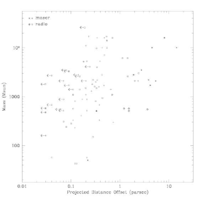
Figure 2: Relation between the distance offset of a tracer from the peak emission of the millimetre source to the mass of the source. Maser sources are depicted with a ‘plus’ symbol, radio continuum sources are depicted with a ‘box’ symbol. Maser and radio sources devoid of millimetre continuum emission have been oriented 45 degrees, such that the masers are indicated by ‘cross’ symbols, whilst the UC HII  regions are indicated by ‘diamonds’. Sources with a zero offset are displayed on the graph as upper limits, determined assuming a $3^{\prime\prime}$ pointing accuracy for the SEST.

6.2 Parameter Analysis

Three physical parameters have been derived from this study, the mass, radius, and the H₂ number density ($n_{H_{2}}$) as listed in Tables 5 and 12.

We examine each of the three parameters, as well as their distances, for each of the four classes of sources (MM, M, MR, R), in order to ascertain whether these populations are similar or not. Histograms for each of the four parameters for each of the sources classes, as well as for the whole sample, have been drawn and are presented in Fig. 3. Class comparative cumulative distributions plots of the mass and the H₂ number density ($n_{H_{2}}$) have also been drawn and are presented in Fig. 4, while the results of the Kolmogorov-Smirnov testing of these two parameters as well as the radius are presented in Table 16.

6.2.1 Histograms of Parameter Distributions

The histograms of the mass distributions (Fig. 3, upper) show that the mm-only sources are less massive than class M, MR, and R sources (i.e. those sources displaying methanol maser and/ or radio continuum emission). The mass of the 392 sources ranges from 0.5 $\times 10^{1}$$M_{\odot}$  to 3.7 $\times 10^{4}$$M_{\odot}$  (both extremes are mm-only sources) with a mean mass of 1.5 $\times 10^{3}$$M_{\odot}$. The median mass of the combined sample of the methanol maser and UC HII  sources is 1.0 $\times 10^{3}$$M_{\odot}$ , with 25% of the distribution between 0.5 and 1.6 $\times 10^{3}$$M_{\odot}$, while the median mass of the mm-only sample is 2.8 $\times 10^{2}$$M_{\odot}$  with 25% of the distribution between 1.3 and 4 $\times 10^{2}$$M_{\odot}$.

Comparatively, the 195 no-ambig sources have masses that range from 1.8 $\times 10^{1}$$M_{\odot}$  to 3.7 $\times 10^{4}$$M_{\odot}$, with a mean mass of 1.9 $\times 10^{3}$$M_{\odot}$. The mean mass of the no-ambig combined maser and radio sample (M + MR + R) is 3.2 $\times 10^{3}$$M_{\odot}$, while for the no-ambig mm-only sources it is 1.1 $\times 10^{3}$$M_{\odot}$.

The histogram of the source radii (Fig. 3, middle) shows that the mm-only cores, as well as the methanol maser cores, generally have smaller radii than those sources with a radio continuum source (i.e. MR and R). With one exception (G0.26+0.01), the mm-only cores have radii less than 2.0 pc, with the majority ($\sim 94\%$) having radii $<1.0$ pc. The radii of all the sources (392) ranges from 0.01 to 2.5 pc, with a mean radius of 0.5 pc. The mean radius of the combined maser and radio sample is 0.7 pc. The mm-only sample has a mean radius of 0.4 pc.

Comparatively, the 195 no-ambig sources have radii ranging from 0.05 to 2.5 pc, with a mean radius of 0.6 pc. The radius of the no-ambig maser and radio combined sample is 0.8 pc. The no-ambig mm-only sources range from 0.05 to 1.7 pc and average 0.5 pc in radius. Faúndez et al. (2004) quote an average radius of $0.4\pm 0.2$ pc from their 1.2 mm continuum emission survey of IRAS  selected sources.

According to the H₂ number density ($n_{H_{2}}$) histogram (Fig. 3, lower), there does not appear to be a correlation between the class of source and its density. The value of $n_{H_{2}}$ for the entire sample ranges from 1.4 $\times~{}10^{3}$ cm^-3, to 1.9 $\times~{}10^{6}$ cm^-3, with an average of 8.7 $\times~{}10^{4}$ cm^-3. The mm-only cores range from 1.6 $\times~{}10^{3}$ cm^-3, to 1.5 $\times~{}10^{6}$ cm^-3, with a mean value of 9.1 $\times~{}10^{4}$ cm^-3. This compares with the work of Faúndez et al. (2004), who obtained an average density of 2.1 $\times~{}10^{5}$ cm^-3 for their sample of IRAS  sources.

The range of the H₂ number density ($n_{H_{2}}$) for the no-ambig sources does not vary, although the mean value of the entire no-ambig sample is 8.4 $\times~{}10^{4}$ cm^-3, whilst for the no-ambig combined maser and radio sample the mean value is 8.0 $\times~{}10^{4}$ cm^-3 and for the mm-only cores the mean value is 7.5 $\times~{}10^{4}$ cm^-3.

The distance histogram (Fig. 3, lowest) does not appear to show any correlation between the type of source and its distance from us. The distances range from 0.4 kpc to 16.7 kpc with a mean distance of 5 kpc. The mode distance is 6 kpc. There is no variation in the distance results for the mm-only sample nor for the no-ambig sample.

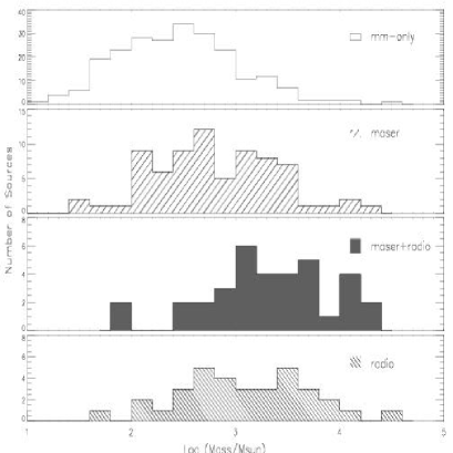
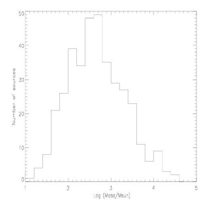
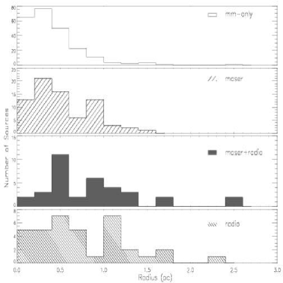
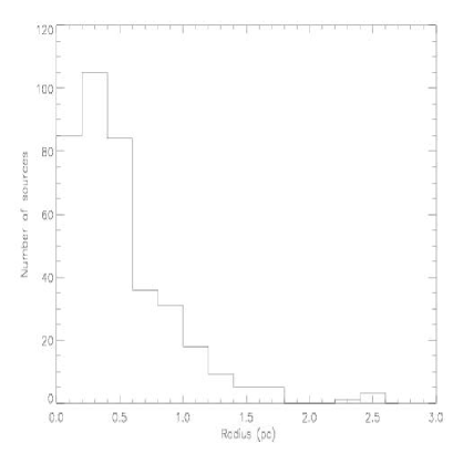
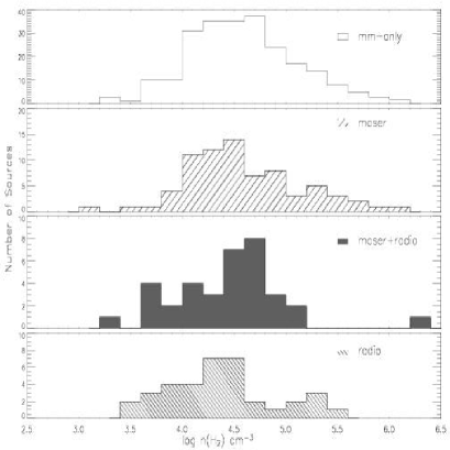
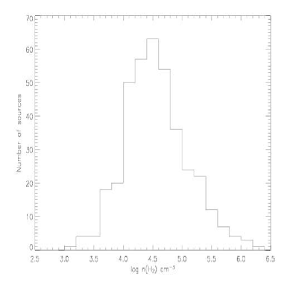
Figure 3: Distributions of the mass, distance, size and number density for all 392 sources detected in this survey (assuming the near distance to 197 sources when the distance is ambiguous). Top Histograms of mass. left: Distribution of the four classes of source (mm-only + maser + maser+radio sources + radio). right: Distribution for all sources. Middle: Radius distributions left: Distribution of the four classes. right: Distribution for all sources. Bottom: H₂ number density ($n_{H_{2}}$) distributions. left: Distribution of the four classes of source. right: Distribution of all sources.

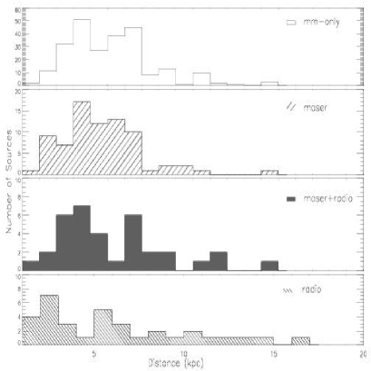
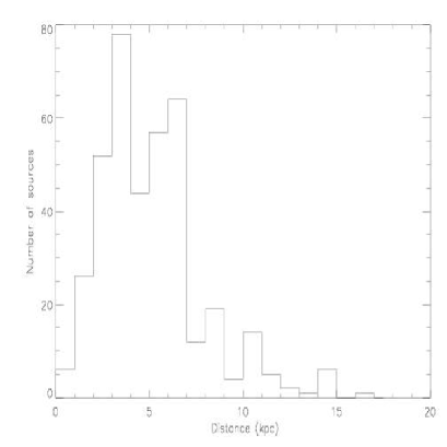
Figure 3: - continued Top: Histograms of distance. left: Distribution of the four classes of source. right: Distribution for all sources.

6.2.2 Kolmogorov-Smirnov Testing of the Cumulative Distributions

The Kolmogorov-Smirnov (hereafter, KS) test was also performed to test the hypothesis that the mm-only cores are drawn from the same parent population as the other three classes of source (M, MR, and R). KS tests were performed for the mass, the H₂ number density, and the radius within each of the four source classes, with the results shown in Table 16.

Generally, in order to conclude that two distributions are not drawn from the same sample, the KS-probabilities must be small, $\leq 0.01$. The null hypothesis, that the samples are drawn from the same population, can only clearly be rejected when comparing the mass of the mm-only sample to the mass of the samples associated with methanol masers and/or radio continuum sources. This is also the case when comparing the radius of the mm-only sample to the radius of samples associated with a radio continuum source (i.e. MR and R). In the case of the H₂ number density, no difference between the samples can be discerned from the data.

As a calibration measure, the KS-test was applied to the class M and R sources. The results, indicate that the likelihood of these sources being from the same parent population is 6.9%. This result is to be expected if the two objects (maser and UC HII) often occur coincident as in the case of the class MR objects, and if the UC HII  region succeeds the maser in the evolution of massive stars.

The cumulative plots of mass, number density and radius, upon which the KS-tests are based, are presented in Figure 4. These illustrate that the mm-only sources are less massive than the other samples, as indicated by the rejection of the null hypothesis in the KS-test. The cumulative plot for the $H_{2}$ number density shows little variation between the four classes. The cumulative plot for the radius shows that the mm-only sources have smaller radii than the other three samples, as well as corroborating the results from the KS-test, that the mm-only sources are distinctly different from those sources associated with a radio continuum source (i.e. MR and R).

The cumulative plots confirm the synopsis presented in the histogram plots (Fig. 3) as discussed in $\S\ref{histograms}$.

Table 16: Results from the KS-test of mass, density ($n_{H_{2}}$), and radius for all four classes of object. Column 1, indicates the parameter being tested. Columns 2 and 3 lists the classes of source being tested. Column 4 gives the resultant KS probability that the objects in columns 2 and 3 are from the same parent population. If this probability is $<$0.01 it is generally concluded that the samples are not drawn from the same population.

Correlation	Source Class	vs Source Class?	KS-prob
(1)	(2)	(3)	(4)
MASS	(MM) mm-only	(M) masers	2.4E-03
		(MR) maser+radio	4.3E-10
		(R) radio	2.6E-05
	(M) maser	(R) radio	6.9E-02
H2 NUMBER	(MM) mm-only	(M) masers	8.9E-01
DENSITY		(MR) maser+radio	2.5E-01
($n_{H_{2}}$)		(R) radio	5.3E-02
	(M) maser	(R) radio	2.1E-01
RADIUS	(MM) mm-only	(M) masers	4.2E-02
		(MR) maser+radio	2.0E-07
		(R) radio	3.7E-04
	(M) maser	(R) radio	3.1E-02

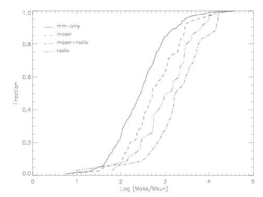
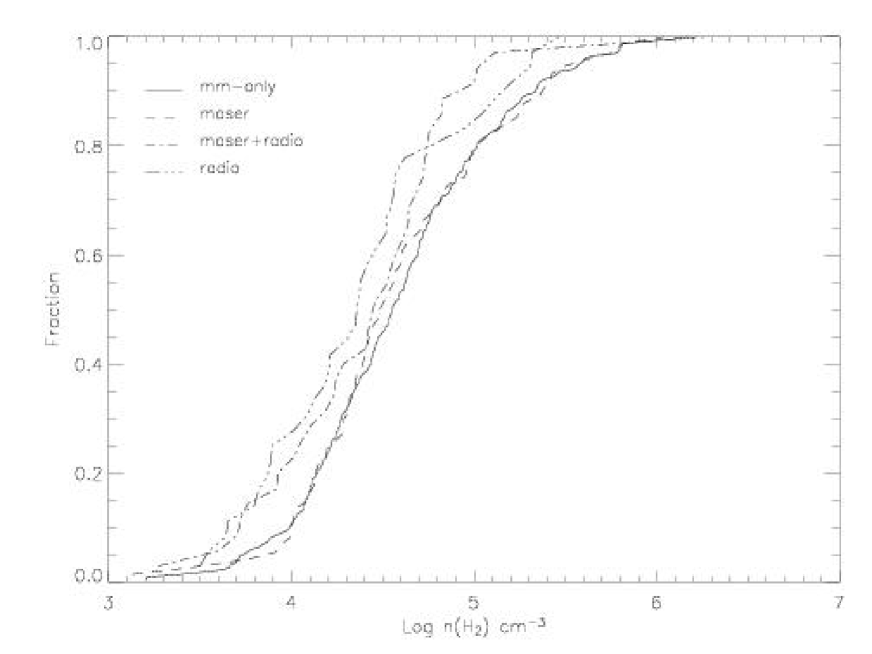
Figure 4: Cumulative Distributions for mass (top) and H₂ number density (bottom)

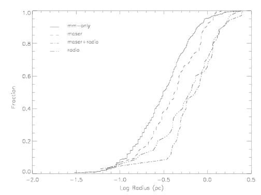
Figure 4: - continued Cumulative Distribution for the radius

6.3 Parameter Correlations

We compare the mass, radius, H₂ number density, and the distance of the sources in Table 5, to examine whether there are correlations between any of these parameters. This analysis is performed on the entire source list (assuming the near distance to 197 sources).

6.3.1 Mass versus Radius

The comparison between the mass and the radius is presented in Figure 5 (top). It is clear that these two parameters are related, with the more massive cores having larger radii, with a best fit of M $\propto$ R^2.2 as discussed further in $\S\ref{discussion}$. This fit has a correlation coefficient of 0.8.

A plot displaying the mass-radius correlation for each source type (MM, M, MR and R) has also been generated and can be found in Fig. 5 (top-right). This plot shows that the mm-only cores tend to dominate the low-mass, low-radius end of the spectrum, but are just as prolific as class M, MR and R at the high-mass, high-radius end. These plots corroborate the results from the mass and radius histograms (Fig. 3) and cumulative plots (Fig. 4), confirming that the mm-only cores can be less massive with smaller radii than sources with masers and/or UC HII  regions (class M, MR, and R).

6.3.2 Mass versus H₂ Number Density

The comparison between the mass and the number density is presented in Figure 5 (middle). There is a much weaker inverse correlation apparent between these two quantities, with M $\propto$ $n_{H_{2}}$^-1.1 i.e., the more massive a core, the lower its average density. The correlation coefficient for this fit is low at 0.2.

There is also no clear distinction between the different categories of source.

6.3.3 H₂ Number Density versus Radius

The relation between the number density and radius is shown in Fig. 5 (lower). Like the mass-radius plot, there is a clear correlation between these two quantities. Denser cores have the tendency to be smaller, on average, with $n_{H_{2}}$ $\propto$ R^-2. This fit has a correlation coefficient of 0.7.

The mm-only cores have a tendency to be both smaller, and have higher densities than the other three categories of source comprising the masers and radio continuum sources.

6.3.4 Mass versus Distance

A comparison between the mass and the distance of the sources is presented in Fig. 5 (bottom). No relation is apparent as would be expected.

The sensitivity limit of our observations, in terms of the lower mass detection limit has been added to the graph as a dotted line.

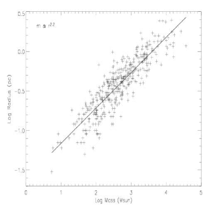
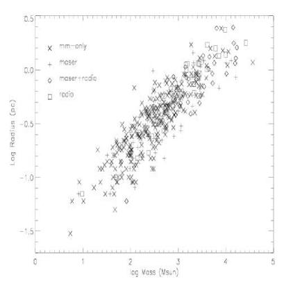
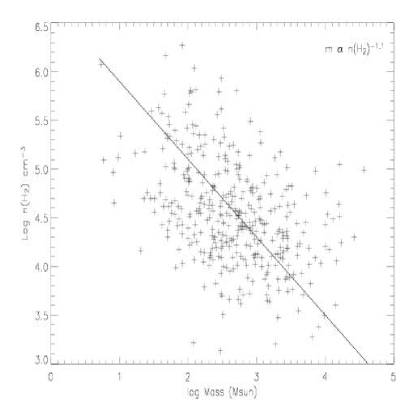
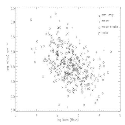
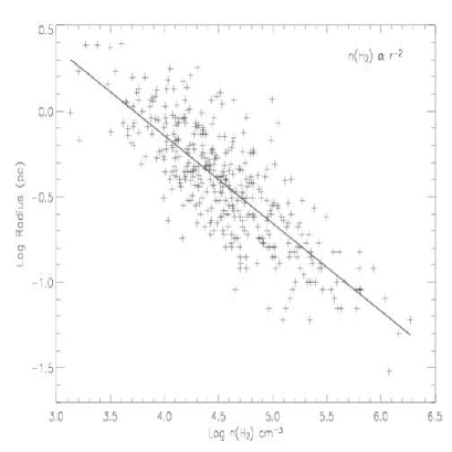
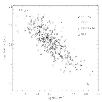
Figure 5: Correlation plots of mass, H₂ number density ($n_{H_{2}}$), radius and distance. The plots on the left correspond to the full source sample (assuming the near distance to 197 sources). The relation best describing the two parameters is printed on the plots. The plots on the right indicate the individual class distributions with a symbol key presented on the plots. Top: correlation plot of the mass and radius of the sources. Middle: Plot of mass and H₂ number density ($n_{H_{2}}$). Bottom: Plot of H₂ number density ($n_{H_{2}}$) and radius.

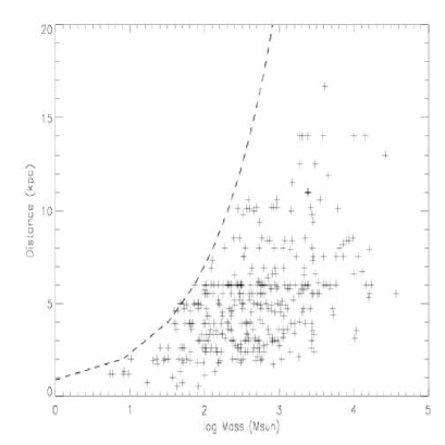
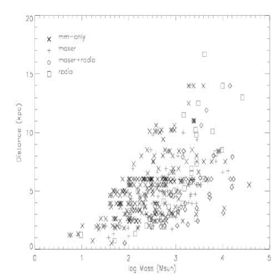
Figure 5: - continued Plot of the mass with distance. The dotted line indicates the 3$\sigma$ mass-sensitivity limit of our survey at 50 mJy.

6.4 Discussion

The physical attributes of mass, radius and $H_{2}$ number density ($n_{H_{2}}$) of each of the four classes of source detected in this survey (MM, R, MR, and R) have been examined to determine whether there are any correlations between each of these parameters, and whether those correlations are source class dependent.

Examination of the mid infrared MSX  images for the SIMBA fields has revealed many sources devoid of mid-IR emission and also many that are associated with mid-IR dark clouds. At a lower limit, we estimate that 30% of the 404 sources detected in this survey have no mid-IR emission, implying that they are cold sources, 90% of which are mm-only cores. Conversely to this, it is not possible to conclusively state that the remaining 70% of sources do have mid-IR emission due to an excess in emission and confusion in many of the infrared images examined.

The histograms (Fig. 3) and cumulative distributions (Fig. 4) show that the mm-only cores are smaller in radius and are also less massive (0.4 pc and 0.9 $\times 10^{3}$$M_{\odot}$  on average) than those cores harbouring a methanol maser and/or an UC HII  region (0.7 pc and 2.5 $\times 10^{3}$$M_{\odot}$  on average). Analysis of the sources with no distance ambiguity confirms the robustness of this result, and the small influence of assuming the near distance for those sources with a distance ambiguity.

The mm-only cores display no evidence of ongoing massive star formation: they are not associated with any compact radio emission signifying the presence of UC HII  regions, nor do they display evidence of H₂O or CH₃OH maser emission. At least 45% of these mm-only cores do not display any mid infrared emission, as detected by the MSX  satellite.

These results lead to two hypotheses about the nature of the mm-only cores. It is possible that they are a precursor to the methanol maser, hence younger, less massive and smaller. Accordingly, these mm-only cores may represent an earlier evolutionary stage to that of cores associated with methanol masers and/or UC HII  regions. That is, they may in fact represent the earliest stage in the formation of massive stars, prior to the onset of methanol maser emission.

However, we can not rule out the possibility that the mm-only cores are simply intermediate mass cores that will give birth to intermediate mass stars (hypothesis 2). Undermining this hypothesis however, is the fact that even the least massive mm-only cores have masses which will support stars in excess of 10 $M_{\odot}$  forming. However, if this hypothesis is true, it suggests that the maximum mass of a star in a cluster is related to the mass of the molecular core from which it is formed.

The mm-only cores may in fact provide examples to support both hypotheses. That is, the smaller, less massive mm-only cores may contain intermediate mass stars in the process of formation, while the larger more massive mm-only cores represent an earlier evolutionary state of massive star formation prior to the onset of methanol maser emission.

Assuming the same temperature (20 K) for all of the cores in the sample introduces an element of uncertainty in the final mass estimates derived. If, for example, we have underestimated the temperature of the radio continuum sources, which typically have temperatures of the order 40 K (c.f. Faúndez et al., 2004), then we have overestimated the mass of the cores by a factor of 2.3 (see Table 4). In this instance the mass ranges of each of the classes of source (MM, M, MR and R) would be comparable. If this were so, then the mm-only cores are colder cores, which are as massive as the methanol maser cores. The mm-only cores are then more likely to represent an earlier stage in the star formation process than those cores with methanol masers or UC HII  regions. Spectral energy distribution modelling in subsequent papers will allow further investigation of the mm-only cores, in particular allowing better estimate of the temperature and hence the mass.

The visual extinction ($A_{v}$) and surface density ($\Sigma$) of 392 sources have been estimated. The visual extinction of our sample varies from 10 to 500 mag with an average of 80 mag, implying a high degree of embedding. The surface density ($\Sigma$) varies from 0.2 to 18.0 kg m^-2 (both extremes are mm-only cores), with an average of 2.8 kg m^-2. Care must be taken in comparing surface densities among source classes, since this parameter depend on how well the source is resolved.

It is clear (c.f. Fig. 5) that the mass and radius of a source are highly correlated, with the more massive cores having larger radii. The H₂ number density and the radius also appear to have a strong relation where the denser cores have smaller radii on average. There is a weak correlation between the mass and the H₂ number density.

The relation between the mass, mean H₂ number density ($n_{H_{2}}$), and the radius of the cores is best described by the following two equations: M $\propto$ R^2.2 and $n_{H_{2}}$ $\propto$ R^-2, where M, R, and $n_{H_{2}}$ are the mass, radius and H₂ number density respectively. Note that these relations are not inconsistent with M $\propto$ $n_{H_{2}}$ R³, despite the substitution of the fits in this formula giving M $\propto$ R, rather then the fitted value of M $\propto$ R^2.2. This is because this formula applies for a specific core, while the relations that we have obtained are for the average properties of the entire sample.

This survey also revealed 20 maser sites and 9 UC HII  regions, which are devoid of millimetre continuum emission (c.f. Table 3). These sources were not specifically targeted in this survey, yet their coordinates fall within the fields mapped by SIMBA.

The positions of 27 of these tracers have been determined via interferometry and hence are accurate to within $1^{\prime\prime}$. The methanol masers are not weaker on average than those methanol masers for which millimetre emission is detected. These 27 maser and radio continuum sources also occur at distances equivalent to those maser and UC HII  regions detected with millimetre continuum emission. Assuming a maximum distance of 16.3 kpc for a particular maser or radio continuum source, then the 3$\sigma$ upper limit at 1.2 mm would imply a mass of 600$M_{\odot}$. Figure 5 (lower) indicates that a particular maser or UC HII  region at this distance would not be detected in the survey with this mass.

Since the majority of sources have masses greater than this, it prompts us to ask why these methanol maser and UC HII  regions are devoid of millimetre continuum emission? Does the lack of millimetre emission suggest that these objects have characteristics dissimilar to those sites associated with massive star formation regions? Does the methanol maser and UC HII  region exist in the later stages of massive star formation, i.e. after the cold core phase, which is no longer detected at millimetre wavelengths? Can massive star formation occur without the presence of these ubiquitous tracers? Or are these objects simply too far away with masses too small to be detected by the sensitivity limit of the SEST? At this time we can not draw a secure conclusion, and further study of these sources is warranted.

7 Conclusions

We have undertaken a millimetre continuum survey of 131 regions of massive star formation, traced by the presence of methanol maser and/or radio continuum emission, using the SIMBA instrument on the SEST. 404 sources are detected in this survey.

Millimetre continuum emission is detected toward all of the methanol maser and UC HII  regions targeted (129). The millimetre continuum emission is offset from the two NM-IRAS  positions however, but this may be attributed to the low resolution offered by IRAS  in pinpointing the peak emission of the central core.

For 20 maser sites, and 9 UC HII  regions, within the surveyed fields, millimetre continuum emission is not detected. Further follow-up work of these objects is required in order to ascertain their nature and the reason for the lack of millimetre emission. It is not clear whether these are simply more distant objects where continuum emission falls below the detection limit.

Also detected in this survey are sources that have no methanol maser or radio continuum emission indicative of MSF. At a lower limit estimate, 45% of these cores are also devoid of mid-IR MSX  emission. The majority of these ‘mm-only’ cores are separate from, and generally offset from, the targeted tracers in the same field.

In total, 253 new mm-only cores have been discovered. Many of the fields contain multiple sources. It is therefore likely that the mm-only cores belongs to the same star formation complex as the methanol maser and UC HII  regions targeted in the study.

The mass, radius and H₂ number density ($n_{H_{2}}$) have been determined from the millimetre flux and distance to the sources, assuming a temperature of 20 K.

Analysis of the mm-only cores reveals that they are generally less massive than those sources with a maser and/or an UC HII  region, and also have smaller radii (c.f. Fig. 3). The results from our analysis leads to two hypotheses about the nature of the mm-only cores. One possibility is that the mm-only core may be a precursor to the methanol maser in the evolutionary sequence of massive stars, the other is that the mm-only cores will simply give birth to intermediate mass stars (i.e. no massive stars that will produce HII  regions). If so, the maximum stellar mass of a cluster is related to the mass of the core from which it forms. Alternatively, the mm-only cores may in fact represent a cross-section of sources supporting both arguments.

We note, that if the cores which only show millimetre emission are systematically cooler than the other classes of source, the temperature assumption of 20 K will introduce a bias, and the different mass distributions we have inferred may not actually occur. In this instance, only the first hypothesis above will apply. A better determination of the temperature of the cores is needed to constrain their masses in order to examine these hypotheses further.

The relation between the mass, H₂ number density ($n_{H_{2}}$), and the radius of the cores is best described by the following two equations: M $\propto$ R^2.2 and $n_{H_{2}}$ $\propto$ R^-2.

Appendix A Presentation of the Images

Maps of the 1.2mm continuum emission detected with the SIMBA instrument on the SEST are presented here. Coordinates of the images are in J2000. For consistency throughout, the methanol maser is depicted as a ‘plus’ symbol, while the radio continuum source (UC HII) is denoted by a ‘box’ symbol. Class MR objects (with both a methanol maser and an UC HII  region) will house both a ‘plus’ and a ‘box’ symbol. The contours are drawn over the 1.2 mm greyscale emission at 10, 30, 50, 70, 90% of the peak emission. Peak emission in each case is presented in Table 5. For the NM-IRAS  sources, (G305.533+0.360 and G305.952+0.555), the IRAS  positions have been included on the images as a black circle asterisk (*) near the centre of the image.

References

- Batrla et al. (1987) Batrla W., Matthews H. E., Menten K. M., Walmsley C. M., 1987, Nature, 326, 49
- Beuther et al. (2002) Beuther H., Schilke P., Menten K. M., Motte F., Sridharan T. K., Wyrowski F., 2002, ApJ, 566, 945
- Blitz (1993) Blitz L., 1993, in Levy E. H., Lunine J. I., eds, Protostars & Planets III . Tucson:Arizona, p. 125
- Bonnell et al. (2004) Bonnell I. A., Vine S. G., Bate M. R., 2004, MNRAS, 349, 735
- Caswell (1996) Caswell J. L., 1996, MNRAS, 283, 606
- Caswell et al. (1995) Caswell J. L., Vaile R. A., Ellingsen S. P., Whiteoak J. B., Norris R. P., 1995, MNRAS, 272, 96
- Egan et al. (1998) Egan M. P., Shipman R. F., Price S. D., Carey S. J., Clark F. O., Cohen M., 1998, ApJL, 494, 199
- Faúndez et al. (2004) Faúndez S., Bronfman L., Garay G., Chini R., Nyman L. A., May J., 2004, A&A, 426, 97
- Frerking et al. (1982) Frerking M. A., Langer W. D., Wilson R. W., 1982, ApJ, 262, 590
- Garay et al. (2003) Garay G., Brooks K. J., Mardones D., Norris R. P., 2003, ApJ, 587, 739
- Garay et al. (2004) Garay G., Faúndez S., Mardones D., Bronfman L., Chini R., Nyman L., 2004, ApJ, 610, 313
- Hildebrand (1983) Hildebrand R. H., 1983, Royal Astron. Soc. Quart. Jrn., 24, 267
- Hunter et al. (1998) Hunter T. R., Neugebauer G., Benford D. J., Matthews K., Lis D. C., Serabyn E., Phillips T. G., 1998, ApJL, 493, L97+100
- Kurtz et al. (1994) Kurtz S., Churchwell E., Wood D. O. S., 1994, ApJS, 91, 659
- Lumsden et al. (2002) Lumsden S. L., Hoare M. G., Oudmaijer R. D., Richards D., 2002, MNRAS, 336, 621
- McKee & Tan (2003) McKee C. F., Tan J. C., 2003, ApJ, 585, 850
- Minier et al. (2005) Minier V., Burton M. G., Hill T., Pestalozzi M. R., Purcell C. R., Garay G., Walsh A. J., Longmore S., 2005, A&A, 429, 945
- Minier et al. (2001) Minier V., Conway J. E., Booth R. S., 2001, A&A, 369, 278
- Motte et al. (2003) Motte F., Schilke P., Lis D. C., 2003, ApJ, 582, 277
- Norris et al. (1993) Norris R. P., Whiteoak J. B., Caswell J. L., Wieringa M. H., Gough R. G., 1993, ApJ, 412, 222
- Ossenkopf & Henning (1994) Ossenkopf V., Henning T., 1994, A&A, 291, 943
- Palagi et al. (1993) Palagi F., Cesaroni R., Comoretto G., Felli M., Natale V., 1993, A&AS, 101, 153
- Panagia & Felli (1975) Panagia N., Felli M., 1975, A&A, 39, 1
- Pestalozzi et al. (2005) Pestalozzi M. R., Minier V., Booth R. S., 2005, A&A, 432, 737
- Phillips et al. (1998) Phillips C. J., Norris R. P., Ellingsen S. P., McCulloch P. M., 1998, MNRAS, 300, 1131
- Reed (2000) Reed B. C., 2000, AJ, 120, 314
- Szymczak & Kus (2000) Szymczak M., Kus A. J., 2000, A&A, 360, 311
- Thompson et al. (2004) Thompson M. A., Hatchell J. H., MacDonald G. H., Millar T. J., 2004, A&A
- Walsh et al. (1998) Walsh A. J., Burton M. G., Hyland A. R., Robinson G., 1998, MNRAS, 301, 640
- Walsh et al. (1997) Walsh A. J., Hyland A. R., Robinson G., Burton M. G., 1997, MNRAS, 291, 261
- Walsh et al. (2003) Walsh A. J., Macdonald G. H., Alvey N. D. S., Burton M. G., Lee J.-K., 2003, A&A, 410, 597
- Williams et al. (2004) Williams S. J., Fuller G. A., Sridharan T. K., 2004, A&A, 417, 115
- Wood & Churchwell (1989a) Wood D. O. S., Churchwell E., 1989a, ApJ, 340, 265
- Wood & Churchwell (1989b) Wood D. O. S., Churchwell E., 1989b, ApJS, 69, 831