Estimating the Porosity of the Interstellar Medium from Three-Dimensional Photoionization Modeling of H ii Regions

Abstract

We apply our three dimensional photoionization code to model Wisconsin H$\alpha$ Mapper observations of the H ii region surrounding the O9.5V star $\zeta$ Oph. Our models investigate the porosity of the interstellar medium around $\zeta$ Oph and the effects of 3D densities on the H$\alpha$ surface brightness and variation in the [N ii] $\lambda$6583/H$\alpha$ line ratio. The $\zeta$ Oph H ii region has a well characterized ionizing source, so it is an excellent starting point for 3D models of diffuse ionized gas. We investigate various hierarchically clumped density structures, varying the overall smoothness within the clumping algorithm. By simulating the observations, we can estimate the porosity of the medium in the vicinity of $\zeta$ Oph and find that within the context of our hierarchically clumped models, around 50% to 80% of the volume is occupied by clumps surrounded by a low density smooth medium. We also conclude that in order for O stars to ionize the diffuse Warm Ionized Medium, the O star environment must be more porous than that surrounding $\zeta$ Oph, with clumps occupying less than one half of the interstellar volume. Our clumpy models have irregular boundaries, similar to observed H ii regions. However, in observed H ii regions it is difficult to identify the precise location of the boundary because of the foreground and/or background emission from the widespread Warm Ionized Medium. This complicates the interpretation of the predicted rapid rise of some emission line ratios near the edge of uniform density H ii regions and combined with the three dimensional clumpy nature of the interstellar medium may explain the apparent lack of distinctive emission line ratios near H i – H ii interfaces.

1 Introduction

The interstellar medium (ISM) is observed to be clumpy on a very wide range of size scales from parsec scale molecular clouds to AU sizes inferred from interstellar scintillation measurements (Hill et al. 2004; Scalo & Elmegreen 2005). This clumpiness is observed to be self-similar over a range of scales with hierarchical or fractal dimensions in the range 2.2 to 2.7 (Sanchez, Alfaro, & Perez 2005). The complex structures are thought to result from mechanical and radiative energy input into the ISM from many processes including stellar winds, supernovae, shocks, photoionization, and cosmic rays. This is reflected in the multi-phase nature of the ISM, where the hot ionized, warm ionized, warm neutral, cold neutral, and molecular gas co-exist. There is considerable debate among theorists regarding the volume filling factors of each phase and the overall structure of the ISM. Over the last decade large multiwavelength surveys of the ISM are providing new high spatial and spectral resolution observations against which observational signatures of theoretical models may be tested. These velocity resolved surveys include neutral gas (Hartmann & Burton 1997), molecular gas (Dame et al. 2001), and diffuse ionized gas (Haffner et al. 2003). The combination of the new datasets and advances in 3D dynamical and radiation transfer simulations now allows for critical testing of global models of the structure and dynamics of the ISM. In this paper we use three-dimensional photoionization models to study the structure of a low density H ii region in the Galaxy on scales of tens of parsecs. This is a first step towards understanding the structure, clumpiness, and ionization of the large scale diffuse ionized gas in the ISM.

Widespread diffuse ionized gas is a significant component of the ISM in the Milky Way (Kulkarni & Heiles 1988; Reynolds 1995) and other galaxies (Rand 1997; Hoopes & Walterbos 2003; Thilker et al. 2002; Collins et al. 2000). The diffuse ionized gas, hereafter referred to as the warm ionized medium (WIM), in the Milky Way is revealed primarily through faint diffuse H$\alpha$ emission and pulsar dispersion measures. The physical characteristics of this gas, including its temperature structure and ionization state, as well as the spectrum of its ionizing sources are probed through analysis of optical forbidden emission lines. The H$\alpha$ data combined with the pulsar data suggest that the WIM has a volume filling factor of about 20% (Reynolds 1991), and is one of the principal components of the ISM. However, there is considerable uncertainty regarding the structure, dynamics, source of ionization, and heating of the WIM (e.g., see recent review by Reynolds, Haffner, & Madsen 2002). The Wisconsin H$\alpha$ Mapper (WHAM) has completed an H$\alpha$ survey of the Northern sky (Haffner et al. 2003) revealing the distribution and kinematics of the WIM in the Galaxy for the first time. Several large regions are also being mapped with WHAM in other lines such as H$\beta$, He i $\lambda$5876, [N ii] $\lambda$6583, [S ii] $\lambda$6716, [O i] $\lambda$6300, and [O iii] $\lambda$5007. The data have revealed the clumpy and filamentary structure of the WIM on large scales, such as the bipolar loop structure in the Perseus Arm which extends $\pm 1$ kpc above and below the Galactic plane (Haffner at al. 1999; Madsen 2004). In addition to the large scale structures, WHAM has mapped several nearby low density H ii regions with sizes of tens of parsecs (e.g., Haffner et al. 1999). Three-dimensional photoionization modeling of these H ii regions may allow us to estimate the structure and porosity of the ISM on these scales. Such models of well-defined H ii regions with known ionizing sources are a first step in modeling the WIM on larger scales with multiple and unidentified ionizing sources.

In this paper we study the three-dimensional structure of the H ii region surrounding the O9.5V star $\zeta$ Oph, incorporating recent WHAM observations in the lines of H$\alpha$, [N ii] $\lambda$6583, and [S ii] $\lambda$6716 (Haffner et al. 1999; Baker et al. 2005). We use the three-dimensional photoionization code of Wood, Mathis, & Ercolano (2004) to model the observed H$\alpha$ intensity and line ratios in order to estimate the clumpiness of the ISM around $\zeta$ Oph. Our models enable us to investigate the penetration and escape of ionizing radiation from clumpy H ii regions into the more widespread WIM. In addition, we study the observational signatures of ionized/neutral interfaces in smooth and clumpy models. Section 2 presents the H$\alpha$ intensity and line ratio maps of the $\zeta$ Oph region, §3 summarizes model predictions for line ratios in H ii regions and at ionized/neutral interfaces, §4 and §5 present smooth and clumpy models for the observations, and we summarize our findings in §6.

2 The $\zeta$ Oph H ii Region

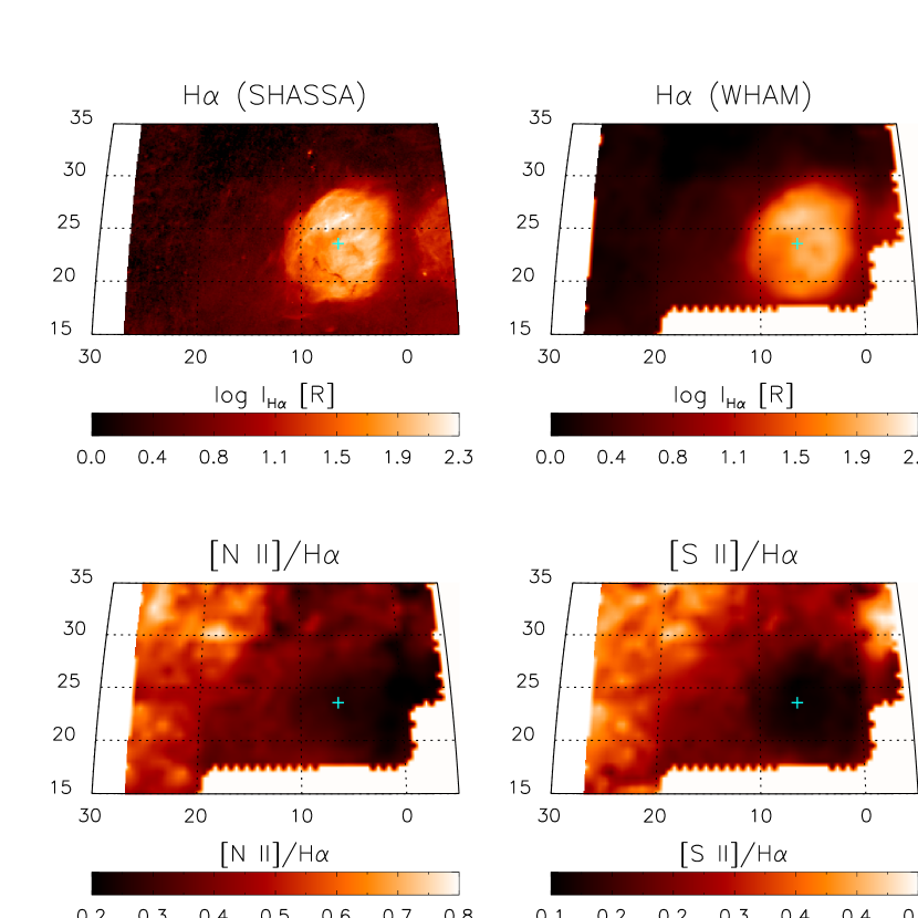
Figure 1: Views of the ionized gas near $\zeta$ Oph (Sharpless 27). The top panels display the logarithm of the H$\alpha$ emission from (left) a moderate-resolution ($\sim 8\arcmin$) image provided by SHASSA (Gaustad et al. 2001; Finkbeiner 2003) and (right) a lower-resolution representation from WHAM. The WHAM spectra have been integrated between $-25$ km s${}^{-1}<v_{\mathrm{LSR}}<+25$ km s^-1 for these images. The lower panels show the (left) [N II]/H$\alpha$ and (right) [S II]/H$\alpha$ ratios of the region. The location of $\zeta$ Oph is denoted by the ’+’ in each panel. Part of the $\delta$ Sco H ii region may be seen at the right edge of the SHASSA image. All four images are displayed with an Aitoff-Hammer projection. The axis labels are Galactic co-ordinates (latitude vs. longitude) in units of degrees.

Figure 1 shows the structure of the H ii region around $\zeta$ Oph. The upper left panel shows the H$\alpha$ intensity from the SHASSA survey (Gaustad et al. 2001; Finkbeiner 2003) with an angular resolution of $0.8\arcmin$. The upper right panel shows the same region at $1^{\circ}$ resolution from the WHAM Northern Sky Survey (Haffner et al. 2003). We have interpolated the irregularly-spaced WHAM observations onto a regular $0\fdg 5\times 0\fdg 5$ grid. The location of $\zeta$ Oph is shown with a cross. The WHAM image shows that the overall structure of the H$\alpha$-emitting gas is remarkably circularly symmetric, although there are strong fluctuations on smaller angular scales as shown in the SHASSA image. Diffuse H$\alpha$ emission associated with the $\zeta$ Oph H ii region is traced out to around $6^{\circ}$ from the star, corresponding to a radius of about 15 pc, before trailing off into more diffuse foreground/background emission toward higher Galactic longitudes (on the left). On the other side of the H ii region the H$\alpha$ intensity becomes confused with that from the $\delta$ Sco H ii region (see Haffner et al. 2003). We do not consider data from this region in our analysis.

The sightline towards $\zeta$ Oph is well studied with many absorption line determinations of interstellar abundances (e.g., Morton 1975; Cardelli et al. 1993, 1994; Howk & Savage 1999). The star itself is catalogued as O9.5V, with an estimated temperature in the range $32\,000<T_{\star}<33\,000$ K (Code et al. 1976; Markova et al. 2004), and a distance of 140 pc (Perryman et al. 1997; Howk & Savage 1999). $\zeta$ Oph has a heliocentric radial velocity of $-10.7$ km s^-1, which is $+3.3$ km s^-1 relative to the local standard of rest. The WHAM data shows that the ionized gas in the H ii region lies at 0 km s^-1. Its proper motion from HIPPARCOS is $13\pm 1$ mas yr^-1 in right ascension and $25.5\pm 0.5$ mas yr^-1 in declination, resulting in a space velocity of $19.3\pm 0.4$ km s^-1 relative to the LSR for a distance of 140 pc. With such a velocity, $\zeta$ Oph travels more than 19 pc in $10^{6}$ years, larger than the 15 pc radius of its own H ii region. Therefore over its lifetime, it appears that $\zeta$ Oph has moved from its birthplace and is now ionizing a different region of the ISM from where it was born. We will return to this point when discussing our photoionization models below.

The H$\alpha$ maps have not been corrected for foreground extinction by interstellar dust that may lie between us and the H ii region. In particular, the dust lane cutting across the lower left quadrant in the SHASSA image is likely in the foreground and not and integral part of the H ii region. Future H$\beta$ observations with WHAM will allow for dust correction and the determination of which features are internal to the H ii region and which are due to foreground dust. However, the [N ii]/H$\alpha$ and [S ii]/H$\alpha$ line ratio maps will not be affected by dust since H$\alpha$, [N ii], and [S ii] are very close in wavelength.

In addition to the H$\alpha$ maps, Fig. 1 shows WHAM line ratio maps of [N ii]/H$\alpha$ and [S ii]/H$\alpha$. These maps show these line ratios increase with distance away from $\zeta$ Oph. Figure 2 shows a scatter plot of H$\alpha$, [N ii]/H$\alpha$ and [S ii]/H$\alpha$ against radial distance from $\zeta$ Oph. The line ratios increase fairly smoothly with increasing distance and do not show the rapid increase expected towards the edge of a uniform density H ii region (see §3). For comparison with models, in the rest of the paper when showing the WHAM data we show the mean radial surface brightness and line ratios and the dispersions about the mean. The mean radial surface brightness is the average value for the H$\alpha$ intensity (or line ratios) in circular annuli centered on $\zeta$ Oph.

3 Interface Emission: Predictions and Observations

One dimensional photoionization models predict rapid increases in the ratios of the projected intensities of [O i], [N ii], and [S ii] relative to H$\alpha$ towards the edge of uniform density H ii regions (e.g., Henney et al. 2005). The increased line ratios occur in the transition region at the edge of the Strömgren sphere where the fraction of neutral gas is increasing and the temperature is rising due to hardening of the radiation field. The wavelength dependence of H⁰ opacity allows the highest energy photons to penetrate the largest distances, resulting in a rising temperature in the interface region (e.g., Osterbrock 1989).

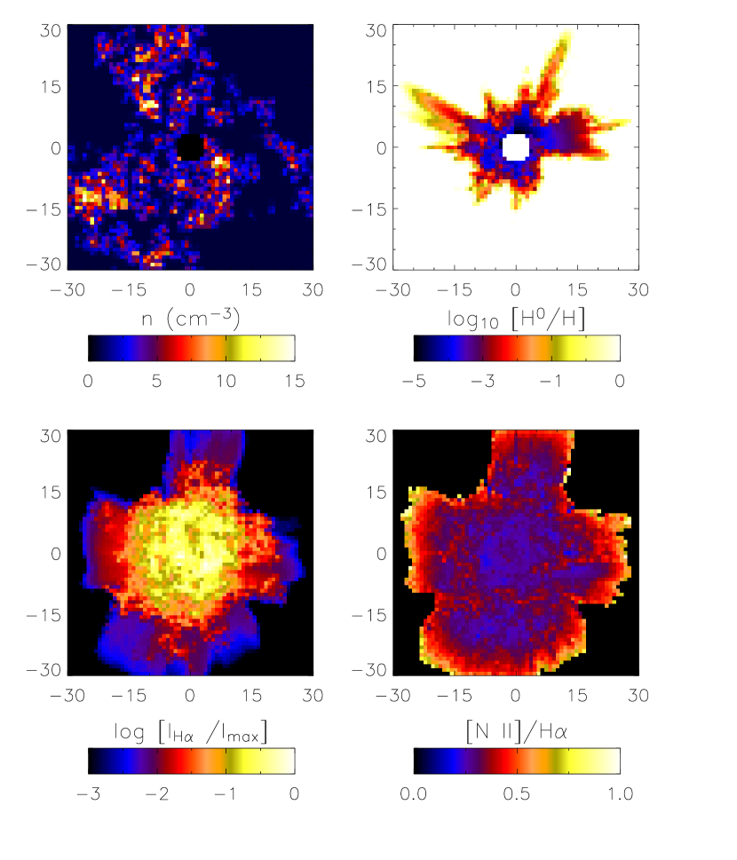
Figure 6: As Fig. 4, but for $N_{1}=64$.

Observations of the diffuse ISM near the Galactic plane show low [O i]/H$\alpha$ line ratios (Reynolds et al. 1998), suggesting that interfaces between ionized and neutral gas have either not been detected or do not contribute significantly to the emission. Photoionization models can explain the low [O i]/H$\alpha$ observations if the WIM is highly ionized (${\rm H}^{0}/{\rm H}<0.1$ throughout), implying that ionizing radiation escapes from fully ionized (i.e., density bounded) H ii regions having few H i – H ii interfaces (e.g., Mathis 1986; Domgoergen & Mathis 1994; Mathis 2000; Sembach et al. 2000). Also, recent work by Giammanco et al. (2004) showed that if a clumpy H ii region is comprised of a mixture of fully and partially ionized spherical clouds, the line ratios increase more slowly with radius than in uniform density, ionization bounded models (e.g., see the radial dependence of [O i]/H$\beta$ in their Fig. 6). This is because the combination of many spherical clouds along a given sightline through the H ii region sample a wide range of ionization parameters and hence the line ratios do not show the rapid increase of uniform, ionization bounded models.

While the predicted rapid rise of temperatures and line ratios at the edges of H ii regions has not been observed (e.g., Pauls & Wilson 1977), gradual rises in the line ratios have been observed with height above the midplane ionizing sources in the Milky Way (Haffner et al. 1999) and several other edge-on galaxies (Rand 1998; Otte et al. 2001, 2002). The elevated [N ii]/H$\alpha$ line ratios observed at large distances from the midplane in the Perseus Arm (Haffner et al. 1999) have been interpreted as due to an extra heat source in addition to photoionization heating (Reynolds et al. 1999). This additional heat source must have the property that it dominates over photoionization heating at low densities. A constant energy source or one that is proportional to $n_{\rm e}$ would suffice, since photoionization heating is proportional to $n_{\rm e}^{2}$. Candidates for the additional heating include photoelectric heating from grains (Reynolds & Cox 1992), magnetic reconnection (Raymond 1992), dissipation of turbulence (Minter & Spangler 1997), shocks and cooling hot gas (Slavin, Shull, & Begelman 1993; Collins & Rand 2001). However, hardening of the radiation field also increases the temperature of photoionized gas and may help to explain in part some of the observed elevated line ratios (e.g., Bland-Hawthorn, Freeman, & Quinn 1997; Elwert 2003; Wood & Mathis 2004).

In this paper we present models for the H ii region associated with $\zeta$ Oph. Additional heating will not be important for this source since the gas density is larger and the line ratios are much lower than observed at high latitude in the Perseus arm. The WHAM observations presented in Figures 1 and 2 show that [N ii]/H$\alpha$ increases away from the source, but does not appear to show the rapid rise at the edge of the H ii region predicted by spherical models with uniform density (see §4.1 below). To understand this behavior we have investigated photoionization models that incorporate various smooth and clumpy density structures for the H ii region and the effects of diffuse foreground/background emission. We discuss the plausibility of the smooth models and the insight three-dimensional models can provide into the structure of the ISM around $\zeta$ Oph and the escape of ionizing photons from H ii regions. Our 3D models produce similar results to those of Giammanco et al. (2004) for radial line ratio gradients, but our 3D radiation transfer allows for shadowing of clumps and multiple clumps along any sightline from the star.

4 Photoionization Models

To model the WHAM observations of the $\zeta$ Oph H ii region, we use the three-dimensional photoionization code described in Wood, Mathis, & Ercolano (2004). This code calculates the 3D ionization and temperature structure for arbitrary geometries and illuminations, keeping track of the ionization structure of H, He, C, N, O, Ne, and S. The opacity is from to H⁰ and He⁰ and we only consider photon energies in the range 13.6 eV to 54 eV. Heating is from photoionization of H and He and cooling is from H and He recombination, free-free emission, and collisionally excited line emission from C, N, O, Ne, and S. The output of our code is the ionization and temperature structure from which we calculate emissivities and intensity maps for the various emission lines we wish to study. A complete description of the code is presented in Wood et al. (2004).

We perform the radiation transfer for stellar and diffuse recombination ionizing radiation on a 65³ linear Cartesian grid. Due to the resolution of our grid, we do not consider emission from cells that are more neutral than ${\rm H}^{0}/{\rm H}\geq 0.25$ (see discussion in Wood et al. 2004). These cells lie towards the edge of the ionized volume and account for less than 20% of the ionized cells in our ionization bounded models. We have constructed intensity and line ratio maps including these cells and find that our results for the [N ii]/H$\alpha$ line ratio maps do not change at the $\sim 5$% level. Moreover, in the cells at the ionization boundary our code is incomplete, since we ignore the effects of dynamics and shocks at the ionization front (Henney et al. 2005). Higher resolution simulations ($128^{3}$ grids) do not appreciably change our results, again at around the $\sim 5$% level.

Our code performs well compared to other photoionization codes in predicting ionization fractions, temperatures, and line strengths. Here we focus on modeling the observed H$\alpha$ intensity and [N ii]/H$\alpha$ maps and do not consider the [S ii]/H$\alpha$ observations. Modeling emission from sulfur is problematic due to the unknown dielectronic recombination rates for S (Ali et al. 1990). In addition we do not consider the effects of dust within the H ii region and note that our temperatures may be slightly higher than calculations that include cooling from more elements (e.g., see Sembach et al. 2000). Since the goal is to investigate the 3D structure of the H ii region by modeling variations in the line ratios towards the edge of the H ii region, ignoring these effects will not change our conclusions on the H ii region density structure. Inclusion of these additional effects will be required for more comprehensive models of future observations of H$\beta$, [O i], [O ii], [O iii], and He i. In particular, we may be able to model data from several H ii regions to place constraints on the S dielectronic recombination rates.

Relative to H, the adopted abundances for He, C, N, O, Ne, and S in our models are 0.1, 140 ppm, 75 ppm, 319 ppm, 117 ppm, and 18 ppm. These are interstellar gas phase abundances from the compilation of Sembach et al. (2000). The ionizing spectrum is taken to be that of a 32 000 K WM-basic model atmosphere from the library of Sternberg, Hoffmann, & Pauldrach (2003). This temperature is within the range estimated for an O9.5V star (see compilation of temperature/spectral type scales and discussion in Harries, Hilditch, & Howarth 2003, Table 4). The WM-basic model atmospheres include the effects of line blanketing and stellar winds (Pauldrach et al. 2001). The ionizing luminosity and density are varied in the models to reproduce the observations of H$\alpha$ and [N ii]/H$\alpha$. The following sections present results for smooth models (with and without density gradients) and three-dimensional, hierarchically clumped models.

4.1 Smooth Spherically Symmetric Models

Our spherically symmetric models are centered on a source with an ionizing photon luminosity $Q$ (s^-1), and the density within the cloud (cm^-3) is given by

$$n(r)=n_{0}\left({{r}\over{1\,{\rm pc}}}\right)^{-p}\;.$$ (1)

where the parameter $p$ controls the radial density gradient within the cloud. In all models (smooth and clumpy) we have left the inner 10% of the grid empty, which prevents the clumping algorithm randomly placing the star in the center of a dense clump. The grid is 60 pc on a side and contains $65^{3}$ cells, while the observed $\zeta$ Oph H ii region is about 40 pc in diameter but has some extensions to greater distances. We have investigated many ($p$, $n_{0}$, $Q$) combinations for ionization and density bounded models and show those that reproduce the overall H$\alpha$ intensity level observed by WHAM. Table 1 summarizes the range of adopted model parameters and the results of the models are compared to the observations in figure 3.

The radial variation of H$\alpha$ and [N ii]/H$\alpha$ may be influenced by the presence of foreground and background emission. This is illustrated in Figure 3 which shows models without (left panels) and with (right panels) the addition of a constant intensity representing foreground/background emission. Both the smooth (shown here) and clumpy models (shown in §4.2) have been convolved with a Gaussian beam to simulate the $1^{\circ}$ angular resolution of WHAM. The diffuse background is taken to be 1.5 R at H$\alpha$ and 0.6 R for the [N ii] simulation. These values provide a good fit to the observations (see Fig. 2) and also are typical for the diffuse interstellar medium near the Galactic latitude ($b=24^{\circ}$) of $\zeta$ Oph (see also Haffner et al. 2003; Madsen 2004). The addition of diffuse foreground/background emission (which is an unavoidable contaminant in real observations) clearly suppresses the very large line ratios that are predicted in the faintest outermost regions ($\sim 20$ pc) of the H ii region. However, even with the addition of foreground/background emission, the uniform density, ionization bounded model (i.e., a classic Strömgren sphere) exhibits a rise in the [N ii]/H$\alpha$ at the edge of the H ii region that is steeper than the observations. The H$\alpha$ intensity gradient in such models is also much steeper at the edge of the ionized region than observed (see also the giant H ii region models of Giammanco et al. 2004). Density bounded or “leaky H ii region” models (Fig. 3) do not exhibit the rapid rise in line ratios because there is no ionized/neutral interface in the simulations (e.g., Mathis 2000; Sembach et al. 2000). The density bounded models shown in Fig. 3 allow about 40% of the ionizing photons to escape. Changing the radial density gradient from uniform ($p=0$) to steeper laws ($p=1$, 2) changes the H$\alpha$ radial surface brightness profile. Models with gradients steeper than $p=1$ do not match the WHAM data. Models with $p=1$ appear to give a reasonable match to the H$\alpha$ intensity, but all the density bounded models underpredict the [N ii]/H$\alpha$ observations.

As mentioned previously, $\zeta$ Oph is at a different radial velocity from its associated H ii region, so models that place the star at the centre of a spherical cloud with radial density gradients seem contrived. A more realistic scenario is that $\zeta$ Oph is ionizing a clumpy medium and we explore 3D cloud geometries and the effects on the intensity and line ratio maps in the next section.

4.2 Hierarchically Clumped Models

There is much evidence for hierarchical structure in the ISM, with surveys of clouds revealing fractal structures (e.g., Elmegreen & Falgarone 1996). We therefore investigate 3D H ii regions which have hierarchically clumped density structures. A 3D hierarchical density structure is created using the algorithm presented by Elmegreen (1997). We use five hierarchical levels and the density in the grid is set as follows. At the first level we randomly cast $N$ points with $x$, $y$, and $z$ coordinates in the range (0,1). At each subsequent hierarchical level we cast $N$ random points around each of the points cast at the previous level. The casting length for the $x$, $y$, and $z$ points at each subsequent level is in the range $\pm\Delta^{(1-H)}/2$, where $H$ is the hierarchical level being cast, and $f=\log N/\log\Delta$ is the fractal dimension of the hierarchical structure. The casting length, $\Delta$, gets smaller for subsequent hierarchical levels. Note that in this description $\Delta$ is dimensionless and we construct the hierarchical grid within a cube with side of unit length. Actual dimensions are constructed by mapping the hierarchical grid onto our 3D density grid, so that the unit cube corresponds to the physical size of our density grid. We use a fractal dimension $f=2.6$, appropriate for interstellar clouds (e.g., Sanchez, Alfaro, & Perez 2005). Using this algorithm, the density of a cell in our grid is proportional to the number of points cast at the final level that lie in the cell. If points are cast beyond the $x$, $y$, or $z$ boundaries of the grid, they are added into the corresponding cells on the opposite side of the grid, e.g. if a point is cast at $x=x_{\rm max}+\epsilon$, we change its coordinate to be $x=\epsilon$ and similarly for $y$ and $z$ coordinates. Figure 4 illustrates this algorithm in 2D for a three tier hierarchical scheme, with four random points cast at each level. The filled in squares are the first castings, diamonds the second level, and crosses at the third level. The dotted lines show overlaid grid cells. We assume that a fraction, $f_{\rm smooth}$, of the average density is present in every cell. The remaining mass is distributed in proportion to the number of crosses that are in each cell.

The smooth component represents unresolved fractal structure that cannot be resolved within our grid. In real nebulae the hot, shocked stellar winds may create very low density regions between the clumps of gas. The resulting clumpy density grid is renormalized so that it has the same mean density structure as the smooth grid. We generally adopt $f_{\rm smooth}=1/3$, but also consider the case where there is zero smooth density component. Our adopted value of $f_{\rm smooth}$ comes from radiation transfer models of the penetration of radiation into turbulent cloud models from hydrodynamic simulations. A value of $f_{\rm smooth}=1/3$ provides a good match for the internal intensity levels between the hydrodynamical simulations and density structures generated with the fractal algorithm (Bethell et al. 2004).

To investigate the clumpiness of the ISM around $\zeta$ Oph we varied $N$ at the first hierarchical level, using $N_{1}=32$, 64, 128, 256, and 512, but keeping $N=32$ at all four subsequent hierarchical levels. With this modification to the clumping algorithm the relation between casting length, $\Delta$, and fractal dimension, $f=\log N/\log\Delta$, is determined assuming $N=32$. Increasing $N_{1}$ at the first level gives a progressively smoother density structure at large spatial scales, but maintains the observed fractal dimension of interstellar clouds on smaller scales. We have not investigated the effects on the ionization structure and line ratios of changing the value $N=32$ at the second and higher hierarchical levels. Increasing $N$ will give a larger dynamic range and finer structure in the hierarchical density grid, because the total number of points used to determine the density is given by the number of castings at the final level, $N_{1}\times N^{4}$. The choice of $N=32$ is not observationally motivated, but is determined by the resolution of our density grid. Using very large values of $N$ is not justified because the fine structure will not be resolved by our grid.

The algorithm produces maximum density contrasts between the densest clumps and the smooth component of 65, 35, 20, 10, for $N_{1}=32$, 64, 128, and 512 respectively. A small $N_{1}$ allows ionizing radiation to penetrate further between the clumps than in a uniform medium (Elmegreen 1997). The fraction of cells that contain only the smooth component of density, without any of the points that were cast randomly, is 65%, 45%, 20%, and 0.1% for these models. If the density in the smooth component is almost zero, ionizing radiation can escape along the empty sightlines into the larger scale ISM.

Having a smooth component of zero density did not significantly change the morphology of our H$\alpha$ maps compared to the $f_{\rm smooth}=1/3$ that we adopt because the emission is dominated by the higher density ionized clumps. For $N_{1}=32$ and $f_{\rm smooth}=1/3$, the smooth component accounts for about 1/3 of the H$\alpha$ intensity level. The smooth contribution to the H$\alpha$ intensity decreases with increasing $N_{1}$. Elmegreen (1997) speculates that much of the volume of a fractal ISM is at very low density, like our models with no smooth component.

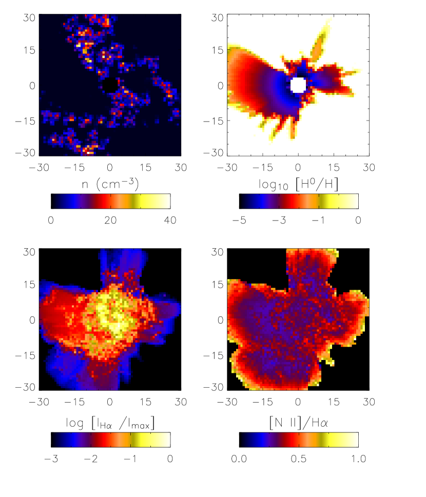
Figure 5: Hierarchically clumped model with $N_{1}=32$ (see text) showing slices through the center of our grid of the number density and hydrogen ionization fraction (upper panels) and the projected H$\alpha$ intensity and projected [N ii]/H$\alpha$ line ratio maps (lower panels). Axes are labeled in parsecs. This model allows for many sightlines from the star that do not intersect a dense clump, producing extended low intensity H$\alpha$ emission which may get lost in strong foreground/background emission.

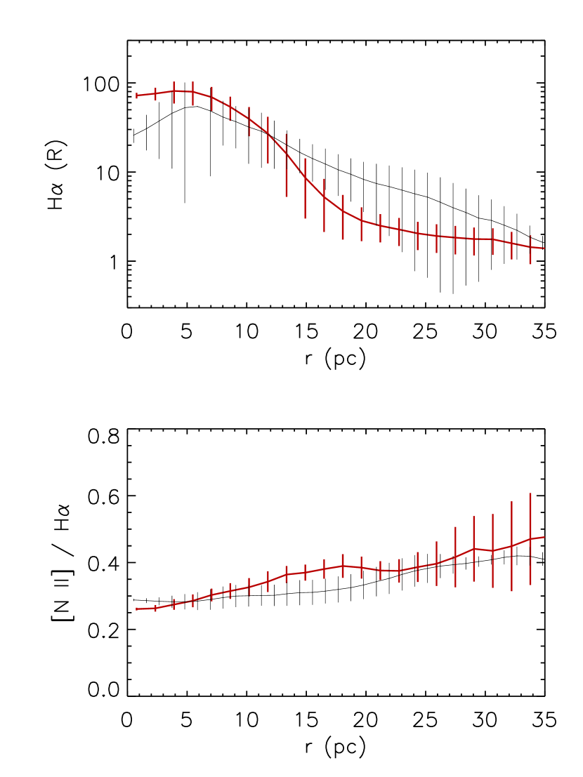
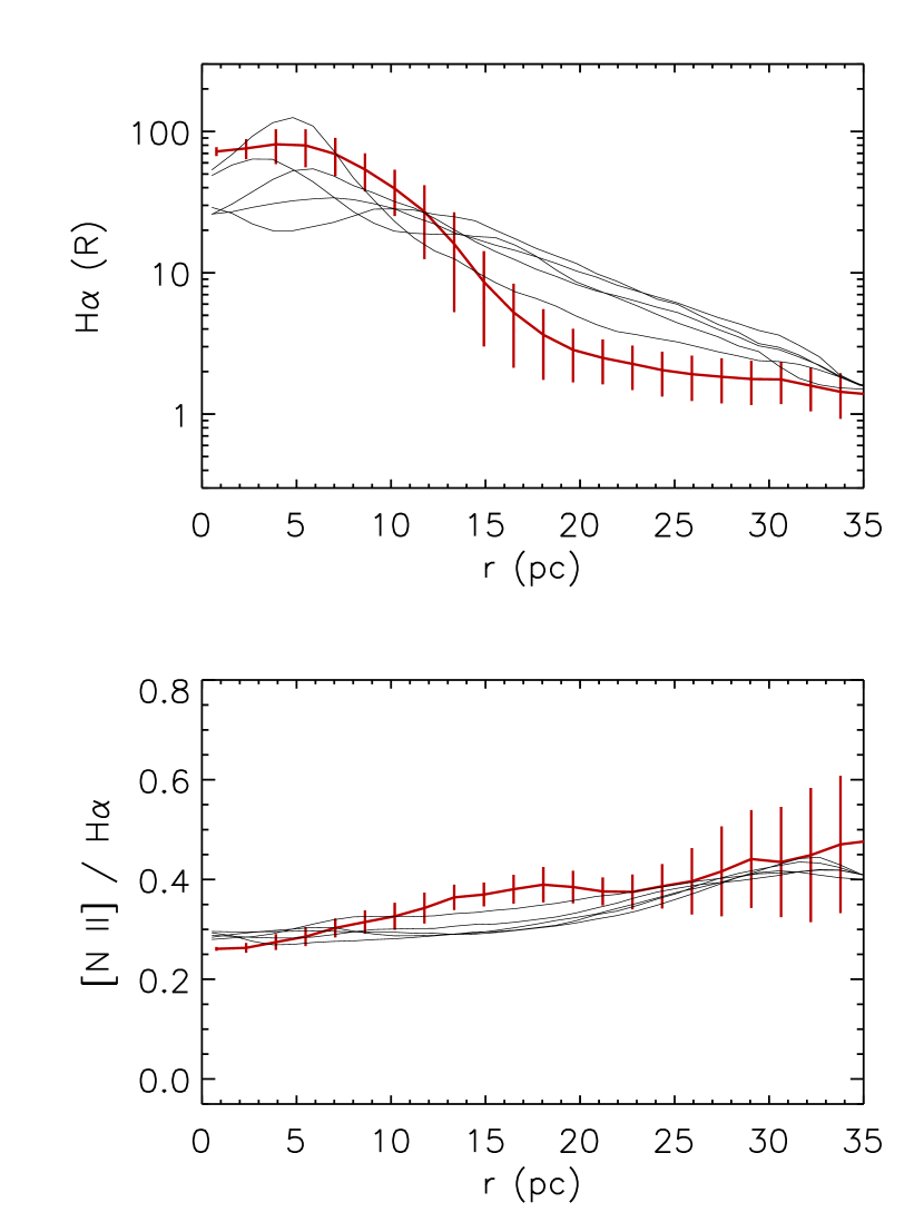
Figure 9: The H$\alpha$ intensity and [N ii]/H$\alpha$ line ratios for the clumpy models with $N_{1}=32$, plotted against the projected offset distance from $\zeta$ Oph. Left panels: red lines show the mean radial intensity and standard deviations measured by WHAM and black lines show the same for one of the $N_{1}=32$ models. A constant intensity of 1.5 R and 0.6 R has been added to the model H$\alpha$ and [N ii] maps to simulate the diffuse foreground/background emission around $\zeta$ Oph. Right panels: red lines again show the WHAM data and the black lines show five different $N_{1}=32$ models — each model has a different randomly cast hierarchical density structure. These models show high H$\alpha$ at large radii due to ionizing photons propagating to large distances through the very porous density structure (see Fig. 5). The [N ii]/H$\alpha$ ratio is systematically lower than observed and the standard deviations of the models are larger than in the WHAM data.

We investigated many different clumpy models for each $N_{1}$ value by changing the random number seed used for setting up the hierarchical density grid. For a given $N_{1}$, each model has a different density structure and hence slightly different H$\alpha$ and [N ii] intensity profile due to the random casting of clumps around the star, but the overall features in the intensity maps are similar. For each $N_{1}$ of our clumpy models, Figures 5 through 8 show one pixel thick slices through one of the density grids and slices showing the hydrogen ionization fraction ${\rm H}^{0}/{\rm H}$. The figures also show the H$\alpha$ intensity and [N ii]/H$\alpha$ line ratio maps, without the addition of uniform foreground/background emission. Figures 9 to 12 show the radial variation of H$\alpha$ and [N ii]/H$\alpha$ with the addition of uniform foreground/background emission. For each $N_{1}$ model, the figures show one model with the standard deviations about the mean and also the radial profiles for simulations of five different density grids.

5 Results

Our models are constrained by the emission line intensities observed at various angles from the star (or distances projected onto the sky) and their dispersions. For all clumpy models the ionizing luminosity is $Q=8\times 10^{47}\,{\rm s}^{-1}$ and the mean density of the H ii region is $n=2\,{\rm cm}^{-3}$. Both the luminosity and density are about 50% smaller than estimated by Elmergreen (1975) from analysis of older H$\alpha$ data from Reynolds et al. (1974). Our estimates for the luminosity and density are well constrained by the intensity and angular extent of the H$\alpha$ data. We find that $N_{1}\sim 64$, followed by coarser clumping on the smaller scales, provides the best fit to the WHAM data. This implies that the real ISM in this direction is not hierarchical, but is smoother on a scale of $\sim 10$ pc than at smaller scales. This result reflects the general circular symmetry in the WHAM H$\alpha$ image in Fig. 1, but the small scale irregularities are not revealed in the WHAM data because of its relatively coarse angular resolution ($1^{\circ}$).

As expected, Figures 5 through 12 show that the clumpy model that most resembles a Strömgren sphere has $N_{1}=512$, since distributing many random points approximates a uniform distribution. This model has a somewhat irregular boundary, but there are no sightlines from the star that do not intersect dense clumps, so overall the model has a very smooth structure and exhibits the large increase in the [N ii]/H$\alpha$ line ratio at the edge of the H ii region. As $N_{1}$ is reduced, the medium becomes less smooth and there are sightlines from the star through which ionizing radiation can traverse large distances before intersecting a clump, or not intersect any clumps. Models with $N_{1}=32$ show a gradual radial decline of the H$\alpha$ intensity. As $N_{1}$ is increased, the fraction of low density sightlines decreases and the H$\alpha$ exhibits a steeper radial gradient. The concavity of the radial H$\alpha$ surface brightness profiles change for larger $N_{1}$ and approach that of the uniform density Strömgren sphere in Figure 3. The trends in our models are similar to the radial surface brightness profiles and line ratios found by Giammanco et al. (2004) in their H ii region models comprising spherical blobs surrounding an ionizing source.

Within the context of our clumping algorithm, we find that models with $N_{1}=32$ produce too much H$\alpha$ at large radii and variations about the mean radial intensity are larger than observed. Models with $N_{1}\geq 256$ resemble Strömgren spheres, producing too steep a gradient of the H$\alpha$ and a rapid rise of [N ii]/H$\alpha$ at the edge of the H ii region and small variations about the mean values. Models with $N_{1}=64$ and 128 provide better matches to the WHAM data in reproducing the observed levels of H$\alpha$ and [N ii]/H$\alpha$, their radial variations, and standard deviations.

While the intensity maps for this low density H ii region model are not very sensitive to the smooth component, the smooth component has a large influence on the ionizing radiation that may escape the H ii region and ionize the larger scale diffuse ionized gas. Models with $N_{1}=32$, 64, and 128 and zero smooth density component ($f_{\rm smooth}=0$) typically allow around 10%–25%, 3%–15%, and 1%–3% respectively of the stellar ionizing photons to escape the H ii region directly along the zero density paths from the star. The large variations in the escape fractions for each $N_{1}$ value are due to the random placing of clumps around the star. Our 3D photoionization models therefore confirm the analysis of Elmegreen (1997) that a fractal ISM will allow for ionizing photons to traverse much larger distances than a smooth density structure. Further clearing of a fractal ISM by feedback from photoionization (Dale et al. 2005) and stellar winds will likely provide an even larger escape fraction from H ii regions than those determined from our models.

Since the widespread H$\alpha$ emission from the Galactic WIM requires about 15% of the ionizing photons from Galactic O stars (Reynolds 1995), it appears that a 3D fractal ISM structure could allow for such leakage from H ii regions. Our hierarchical density models for the ISM around $\zeta$ Oph with $N_{1}=64$ and 128 typically provide escape fractions of less than 15%, and even lower if the density in the smooth component is not zero. Therefore, the ionizing sources responsible for powering the WIM in the Galaxy must reside in regions of the Galaxy that are more porous than the region around $\zeta$ Oph. Perhaps their environment has been shaped more by turbulent motions or are regions cleared out by stellar winds, thus enabling the escape of ionizing photons. Future models of WHAM observations of other H ii regions will enable us to determine whether the porosity levels for the ISM around $\zeta$ Oph are typical.

Our models placed the star at the center of a fractal cloud, so models where the star is at the edge of the cloud will allow for larger leakage, since the cloud no longer covers the whole sky as seen from the star. The major question from this work relating to ionization of the diffuse ionized gas is what is the density of the smooth component in fractal models? We cannot determine how much H$\alpha$ emission from the WIM comes from an extensive, relatively smooth component and how much is from ionized clumps and the ionized faces of clouds. Further progress to answer this question may be made by conducting photoionization simulations on the 3D density grids being produced by global models of the ISM (e.g., de Avillez & Berry 2001). Such models predict the ISM density structure and the locations of ionizing sources and their validity may be tested against observations through 3D photoionization simulations.

6 Summary

We have presented smooth and clumpy 3D photoionization models for the $\zeta$ Oph H ii region. We find that a star with $T=32\,000$ K and ionizing photon luminosity $Q=8\times 10^{47}\,{\rm s}^{-1}$ and mean density of the H ii region of $n\approx 2\,{\rm cm}^{-3}$ reproduce the observations. These numbers are well constrained by the WHAM data. The stellar temperature and ionizing luminosity are remarkably close to recent determinations of stellar properties for O9.5V stars (Martins et al. 2005, Table 4). Larger densities require a larger ionizing luminosity to match the extent of the H ii region, but then the H$\alpha$ values are larger than observed. Smaller densities have the opposite effect, requiring a lower ionizing luminosity to match the extent of the H ii region, but then the simulated H$\alpha$ intensity is much smaller than observed.

Smooth models that best match the observations are density bounded and have a radial density gradient that falls off no faster than $r^{-1}$. However, the velocity offset between $\zeta$ Oph and its H ii region suggest that these uniform models are unrealistic as they require the chance alignment of the star at the center of the cloud. The inclusion of foreground/background emission suppresses the rapid rise in the [N ii]/H$\alpha$ line ratio predicted at the edge of uniform Strömgren spheres.

Hierarchically clumped models, which reproduce the observed fractal structure in the ISM, also reproduce the H$\alpha$ surface brightness and the shallow gradient of [N ii]/H$\alpha$ away from $\zeta$ Oph. The best models suggest that around 20% ($N_{1}=128$) to 50% ($N_{1}=64$) of the H ii region volume is occupied by gas distributed in a smooth component or at very low density, with the remainder in clumps. Three-dimensional models that are more uniform do not match the observations.

The large, low density regions in 3D models could allow ionizing photons to escape at levels that sustain the ionization of the large scale diffuse ionized gas in the Galaxy. However, the escape fractions from our preferred clumpy models for $\zeta$ Oph are less than the 15% escape fraction required to ionize the WIM. Therefore we conclude that the stars responsible for ionizing the WIM must reside in regions of the ISM that are more porous than that surrounding $\zeta$ Oph, possibly evacuated by supernovae and/or stellar winds. A more detailed investigation into the leakage of ionizing photons to the WIM requires consideration of dynamical clearing and the time evolution of the ionizing luminosity of O stars.

Future work will include more comprehensive modeling of the planned mapping observations of $\zeta$ Oph in additional emission lines. The WHAM survey has mapped out several other low emission measure H ii regions and 3D modeling will allow us to test whether the porosity values we estimate for the $\zeta$ Oph region are common in other regions. Modeling the [S ii] emission from many such regions may help to place constraints on the as yet unknown dielectronic recombination rates for sulfur. From a theoretical perspective, global dynamical models of the ISM can be tested by applying 3D photoionization codes and comparing their observational signatures with the high resolution observations now available of diffuse ionized gas in our own and other galaxies.

Table 1: Smooth Model Parameters

$n_{0}$	$p$	$R_{\rm max}$	$Q$	Ionization
$({\rm cm}^{-3})$		(pc)	$(10^{47}\,{\rm s}^{-1})$	bounded?
2.0	0	30	8	yes
2.0	0	18	20	no
7.5	1	18	20	no
98.0	2	18	20	no

Figure 2: WHAM data showing the variation of H$\alpha$, [N ii]/H$\alpha$, and [S ii]/H$\alpha$ as a function of radius from $\zeta$ Oph. Notice the relatively smooth increase of the line ratios with distance and the absence of the rapid increase expected at the edge of a uniform density Strömgren sphere.

Figure 3: Smooth models without (left) and with (right) the addition of foreground/background emission. The heavy solid line shows the mean radial intensity and standard deviation (error bars) measured by WHAM. The lighter lines show the models from Table 1: uniform ionization bounded (solid), density bounded: uniform (dotted), $1/r$ density (dashed), and $1/r^{2}$ density (dot-dashed).

Figure 4: A 2D illustration of the fractal generating algorithm for a three tier scheme. Four random points (filled in squares) are cast at the first level. At each subsequent level a further four points are cast around each of the points cast at the previous level. In this example there are a total of 16 points (diamonds) cast at the second level, and a total of 64 points (crosses) cast at the third level. The density in each cell in the grid (dashed lines) is proportional to the number of crosses in the cell. In our 3D models we use a five tier scheme with $N_{1}=32$, 64, 128, or 512 points cast at the first level and at each subsequent level we cast $N=32$ points around each of the points cast at the previous level. Increasing $N_{1}$ results in a overall smoother medium (see Figs. 5 through 8).

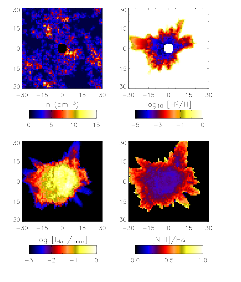
Figure 7: As Fig. 4, but for $N_{1}=128$.

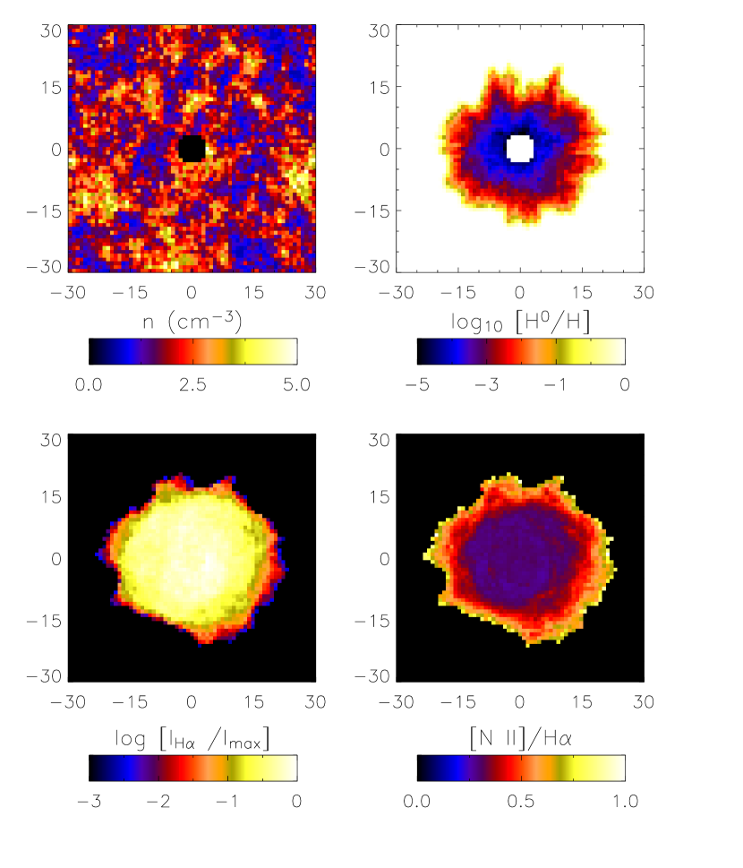
Figure 8: As Fig. 4, but for $N_{1}=512$. Notice how much more circularly symmetric the ionized region (upper right) is than in Fig. 5, because the many points in the initial casting tend to fill space unifromly.

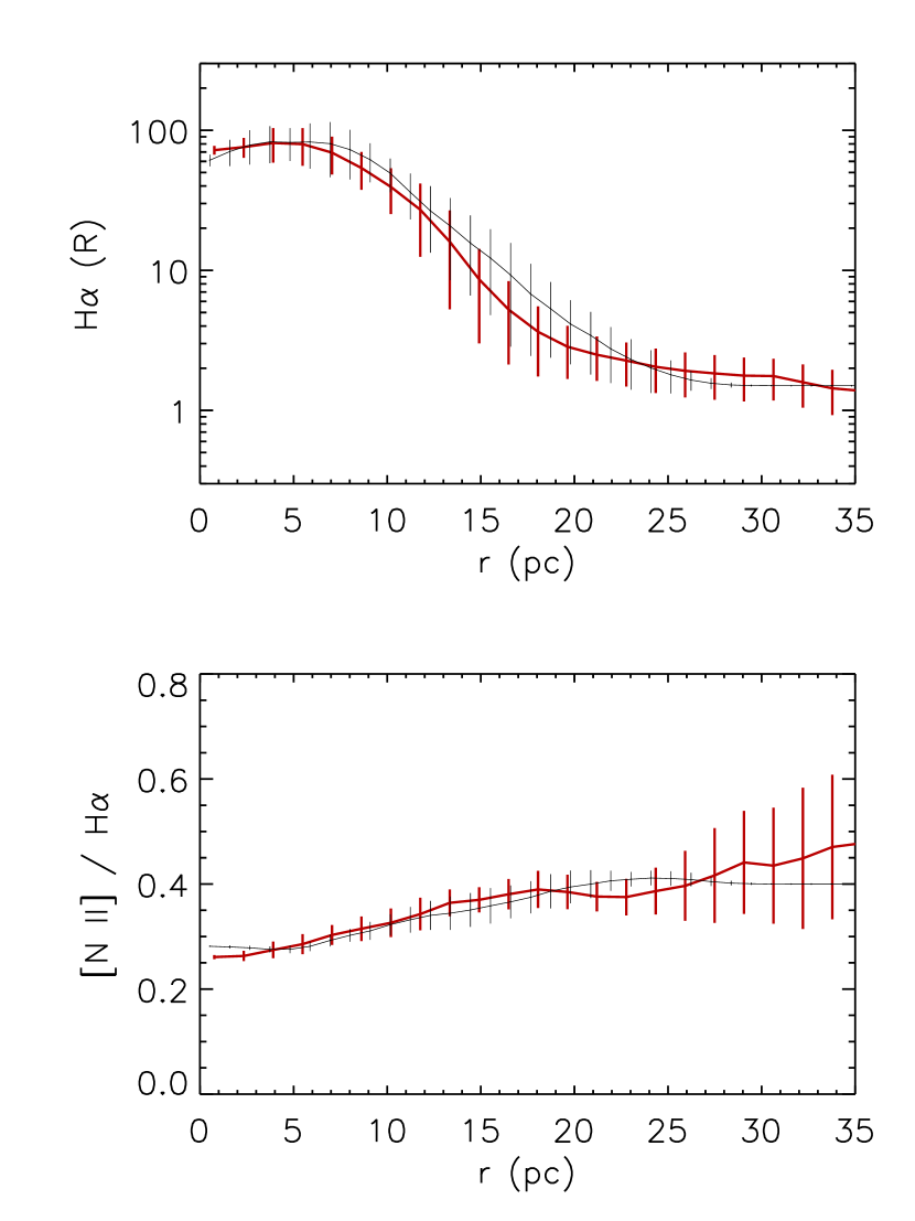
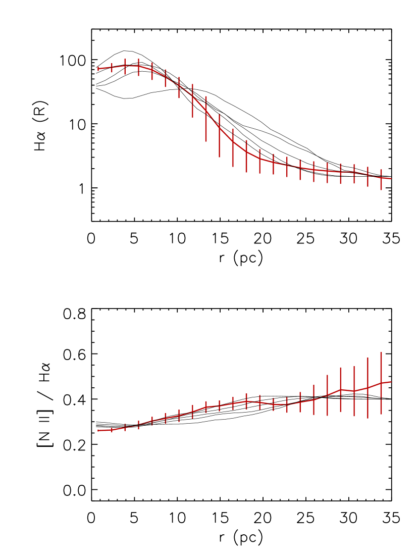
Figure 10: As Fig. 8, but for $N_{1}=64$.

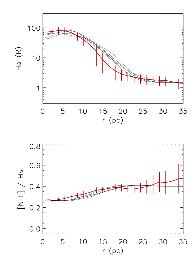
Figure 11: As Fig. 8, but for $N_{1}=128$.

Figure 12: As Fig. 8, but for $N_{1}=512$. This clumpy model closely resembles the uniform density, ionization bounded H ii region since this model has the smoothest density structure of the 3D models presented (see Figs. 5 through 8).

References

- Ali et al. (1991) Ali, B., Blum, R.D., Bumgardner, T.E., Cranmer, S.R., Ferland, G.J., Haefner, R.I., & Tiede G.P. 1991, PASP, 103, 1182
- Baker et al. (2005) Baker, R.I., Haffner, L.M., Reynolds, R.J., & Madsen, G.J. 2005, BAAS, 205, 139.03
- Bethell et al. (2004) Bethell, T.J., Zweibel, E.G., Heitsch, F., & Mathis, J.S. 2004, ApJ, 610, 801
- Bland-Hawthorn et al. (1997) Bland-Hawthorn, J., Freeman, K.C., & Quinn, P.J. 1997, ApJ, 143, 155
- Cardelli et al. (1994) Cardelli, J.A., Sofia, U.J., Savage, B.D., Keenan, F.P., & Dufton, P.L. 1994, ApJ, 420, L29
- Cardelli et al. (1993) Cardelli, J.A., Mathis, J.S., Ebbets, D.C., & Savage, B.D., 1993, ApJ, 402, L17
- Code et al. (1976) Code, A.D., Bless, R.C., Davis, J., & Brown, R.H. 1976, ApJ, 203, 417
- Collins & Rand (2001) Collins, J.A., & Rand, R.J. 2001, ApJ, 551, 57
- Collins et al. (2000) Collins, J.A., Rand, R.J., Duric, N., & Walterbos, R.A.M. 2000, ApJ, 536, 645
- Dale et al. (2005) Dale, J.E., Bonnell, I.A., Clarke, C.J., & Bate, M.R. 2005, MNRAS, 358, 291
- Dame et al. (2001) Dame, T.M., Hartmann, D., & Thaddeus, P. 2001, ApJ, 547, 792
- de Avillez & Berry (2001) de Avillez, M. A., & Berry, D.L. 2001, MNRAS, 328, 708
- Domgoergen & Mathis (1994) Domgoergen, H., & Mathis, J.S. 1994, ApJ, ApJ, 428, 647
- Elmegreen (1997) Elmegreen, B.G. 1997, ApJ, 477, 196
- Elmegreen & Falgarone (1996) Elmegreen, B.G., & Falgarone, E. 1996, ApJ, 471, 816
- Elmergreen (1975) Elmergreen, B.G. 1975, ApJ, 198, L32
- Elwert (2003) Elwert, T., 2003, PhD Thesis, University of Bochum
- Finkbeiner (2003) Finkbeiner, D. 2003, ApJS, 146, 407
- Gaustad et al. (2001) Gaustad, J.E., McCullough, P.R., Rosing, W., & Van Buren, D. 2001, PASP, 113, 1326
- Giammanco et al. (2004) Giammanco, C, Beckman, J.E., Zurita, A., & Relano, M. 2004, A&A, 424, 877
- Haffner et al. (2003) Haffner, L.M., Reynolds, R.J., & Tufte, S.L., Jaehnig, K.P., & Percival, J.W. 2003, ApJS, 149, 405
- Haffner et al. (1999) Haffner, L.M., Reynolds, R.J., & Tufte, S.L. 1999, ApJ, 523, 223
- Harries et al (2003) Harries, T.J., Hilditch, R.W., & Howarth, I.D. 2003, MNRAS, 339, 157
- Hartmann & Burton (1997) Hartmann, D., & Burton, W.B. 1997, “Atlas of Galactic Neutral Hydrogen,” Cambridge University Press
- Henney et al. (2005) Henney, W.J., Arthur, S.J., Williams, R.J.R., & Ferland, G.J. 2005, ApJ, 621, 328
- Hill et al. (2005) Hill, A.S., Stinebring, D.R., Asplund, C.T., Berkwick, D.E., Everett, W.B., & Hinkel, N.R. 2005, ApJ, 619, L171
- Hoopes & Walterbos (2003) Hoopes, C.G., & Walterbos, R.A.M. 2003, ApJ, 586, 902
- Howk & Savage (1999) Howk, J.C., & Savage, B.D. 1999, ApJ, 517, 746
- Kulkarni & Heiles (1988) Kulkarni, S.R., & Heiles, C. 1988, in Galactic & Extragalactic Radio Astronomy (2nd edition) (New York: Springer-Verlag), 95
- Madsen (2004) Madsen, G. 2004, PhD Thesis, University of Wisconsin-Madison
- Markova et al. (2004) Markova, N., Puls, J., Repolust, T., & Markov, H. 2004, A&A, 413, 693
- Martins et al. (2005) Martins, F., Schaerer, D., & Hillier, D.J. 2005, A&A, in press, astro-ph/0503346
- Mathis (2000) Mathis, J. S. 2000, ApJ, 544, 347
- Mathis (1986a) Mathis, J. S. 1986, ApJ, 301, 423
- Minter & Spangler (1997) Minter, A. H., & Spangler, S. R., 1997, ApJ, 458, 194
- Morton (1975) Morton, D.C. 1975, ApJ, 197, 85
- Otte et al. 2002 (2002) Otte, B., Gallagher, J.S., & Reynolds, R.J. 2002, ApJ, 572, 823
- Otte et al. 2001 (2001) Otte, B., Reynolds, R.J., Gallagher, J.S., & Ferguson, A.M.N. 2001, ApJ, 560, 207
- Osterbrock (1989) Osterbrock, D. E. 1989, Astrophysics of Gaseous Nebulae and Active Galactic Nuclei, University Science Books, Mill Valley, CA
- Pauldrach et al. (2001) Pauldrach, A.W.A., Hoffmann, T.L., & Lennon, M. 2001, A&A, 375, 161
- Pauls & Wilson (1977) Pauls, T., & Wilson, T.L. 1977, A&A, 60, L31
- Perryman et al. (1997) Perryman, M.A.C., et al. 1997, A&A, 323, L49
- Rand (1998) Rand, R. 1998, ApJ, 501, 137
- Raymond (1992) Raymond, J.C. 1992, ApJ, 384, 502
- Reynolds, Haffner, & Madsen (2002) Reynolds, R. J., Haffner, L.M., & Madsen, G.J. 2002, in Galaxies in the Third Dimension, ASP Conf. Ser., 282, eds M.Rosado, L. Binette, & L. Arias (San Francisco: ASP), 31
- Reynolds, et al. (1998) Reynolds, R. J., Hausen, N.R., Tufte, S.L. & Haffner, L.M. 1998, ApJ, 494, L99
- Reynolds, et al. (1998) Reynolds, R. J., Haffner, L. M., & Tufte, S.L. 1999, ApJ, 525, L21
- Reynolds (1995) Reynolds, R.J. 1995 in The Physics of the Interstellar Medium and Intergalactic Medium, ASP Conf. Ser., 80, eds, A. Ferrara, C.F. McKee, C. Heiles, & P.R. Shapiro (San Francisco: ASP), 388
- Reynolds & Cox (1992) Reynolds, R. J., & Cox, D.P. 1992, ApJ, 400, L33
- Reynolds (1991) Reynolds, R. J. 1991, ApJ, 372, L17
- Reynolds, et al. (1974) Reynolds, R. J., Roesler, F.L., & Scherb, F. 1974, ApJ, 179, 651
- Sanchez, Alfara, & Perez (2005) Sanchez, N., Alfaro, E.J., & Perez, E. 2005, ApJ, in press, astro-ph/0501573
- Scalo & Elmegreen (2004) Scalo, J., & Elmegreen, B.G. 2004, ARA&A, 42, 275
- Sembach et al. (2000) Sembach, K.R., Howk, J.C., Ryans, R.S.I., & Keenan, F.P. 2000, ApJ, 528, 310
- Slavin et al. (1993) Slavin, J.D., Shull, J.M., & Begelman, M.C. 1993, ApJ, 407, 83
- Sternberg, Hoffmann, & Pauldrach (2003) Sternberg, A., Hoffmann, T.L., & Pauldrach, A.W.A. 2003, ApJ, 599, 1333
- Thilker et al. (2002) Thilker, D.A., Walterbos, R.A.M., Braun, R., & Hoopes, C.G. 2002, AJ, 124, 3118
- Wood & Mathis (2004) Wood, K., & Mathis, J.S. 2004, MNRAS, 353, 1126
- Wood et al. (2004) Wood, K., Mathis, J.S., & Ercolano, B. 2004, MNRAS, 348, 1337