On the effective particle acceleration in the paraboloidal magnetic field

Abstract

The problem of the efficiency of particle acceleration for paraboloidal poloidal magnetic field is considered within the approach of steady axisymmetric MHD flow. For the large Michel magnetization parameter $\sigma$ it is possible to linearize the stream equation near the force-free solution and to solve the problem self-consistently as was done by Beskin, Kuznetsova & Rafikov (1998) for monopole magnetic field. It is shown that on the fast magnetosonic surface the particle Lorentz factor $\gamma$ does not exceed the standard value $\sigma^{1/3}$. On the other hand, in the supersonic region the Lorentz factor grows with the distance $z$ from the equatorial plane as $\gamma\approx(z/R_{\rm L})^{1/2}$ up to the distance $z\approx\sigma^{2}R_{\rm L}$, where $R_{\rm L}=c/\Omega_{\rm F}$ is the radius of the light cylinder. Thus, the maximal Lorentz factor is $\gamma_{\rm max}\approx\sigma$, which corresponds to almost the full conversion of the Poynting energy flux into the particle kinetic one.

1 Introduction

An activity of many astrophysical sources (pulsars, active galactic nuclei) is associated with the presence of a strong magnetic field ($\sim 10^{4}$ G for AGNs and $\sim 10^{12}$ G for pulsars) surrounding the rapidly rotating object and a relativistic particle outflow. Convenient way to characterize such flows is to introduce the magnetization parameter $\sigma$, as was first done by Michel (1969):

$$\sigma=\frac{e\Omega\Psi_{\rm tot}}{4\lambda m_{\rm e}c^{3}}.$$ (1)

Here $\Psi_{\rm tot}$ is the total magnetic flux, and $\lambda=n/n_{\rm GJ}$ is the multiplication parameter of plasma ($|e|n_{\rm GJ}={|\mbox{\boldmath$\Omega$}}\textbf{B}|/2\pi c$ is the Goldreich-Julian charge density). The magnetization parameter characterizes the quotient of electro-magnetic flux to particle kinetic energy flux near the surface of an object. The so-called $\sigma$-problem, i.e., the problem of transformation of electro-magnetic energy into particle kinetic one, appears while one trying to explain an effective particle acceleration in the magnetic field.

Indeed, the flow in the vicinity of different objects is assumed to be strongly magnetized at its origin. In spite of the lack of observational data near the surface of radio pulsars, theoretical modeling predicts that the wind in this region has a composition $\sigma\gg 1$ (Michel, 1991; Beskin, Gurevich & Istomin, 1993). The same can be said about the AGNs (Begelman, Blandford & Rees, 1984). As for the Lorentz factor $\gamma$, at least for the blazars, the deficiency of a soft X-ray bump in their spectrum, which would be produced by the Comptonized direct radiation from the disc, is a reason to exclude the presence of particles with $\gamma>5$ in the near zone of an object (Sikora et al, 2005). On the other hand, at large distance from a pulsar, observations and modeling allow us to determine the magnetization parameter $\sigma\approx 10^{-3}$ (Kennel & Coroniti, 1984). Observations of quasars and active galactic nuclei give $\sigma\leq 1$ and $\sigma\ll 1$ (Sikora et al, 2005).

Up to now the axisymmetric stationary MHD approach gave the inefficient particle acceleration beyond the fast magnetosonic surface (Beskin, Kuznetsova & Rafikov, 1998; Bogovalov, 1997; Begelman & Li, 1994). This seemed to be a general conclusion for any structure of a flow, however a lack of acceleration in the supersonic region was rather the consequence of monopole field (Spitkovsky & Arons, 2004; Thomson, Chang, & Quataert, 2004). The reconnection in a striped wind was discussed as one of possible acceleration scenarios (Coroniti, 1990; Lyubarsky & Kirk, 2001; Kirk & Lyubarsky, 2001); however, this mechanism can account only for the non-axisymmetric part of a Poynting flux. Besides, for the Crab pulsar, Lyubarsky & Kirk (2001) had shown that effective acceleration may take place only beyond the standing shock. Another acceleration process can be connected with possible restriction of the longitudinal current, and thus the appearance of a light surface $|\mathbf{E}|=|\mathbf{B}|$ at the finite distance from a central object. In this case the effective energy conversion and the current closure takes place in the boundary layer near the light surface (Beskin, Gurevich & Istomin, 1993; Chiueh, Li & Begelman, 1998; Beskin & Rafikov, 2000).

In this work we are trying to solve the problem of particle acceleration self-consistently within the approach of stationary axisymmetric magnetohydrodynamics. We regard particle inertia to be a small disturbance to the force-free flow. This allows us to linearize stream equation and to find the disturbance to the magnetic flux, which corresponds to the finite mass of particles. Given that we can find the growth of a Lorentz factor. In the work of Beskin, Kuznetsova & Rafikov (1998) the Michel’s monopole solution was taken as the zero approximation to the flow. For this structure of the magnetic field, the Lorentz factor was found to be $\sigma^{1/3}$ on the fast magnetosonic surface, which was located at the finite distance unlike the force-free limit. Beyond that singular surface the acceleration turned out to be ineffective. Treating the problem numerically, Bogovalov (1997) and later Komissarov (2004) also has got inefficient acceleration and collimation for monopole outflow. Now we took the flow near another force-free solution, i.e., Blandford’s paraboloidal magnetic field (Blanford, 1976). The obvious difference of this zero-approximation in comparison with monopole solution is a well-collimated flow even in the force-free limit.

In Section 2 we remind the trans-field and Bernoulli equations describing the stationary axisymmetric ideal outflow. After formulating the problem in Section 3, it is shown in Section 4 that the fast magnetosonic surface (FMS) is located at the distance $r_{\rm F}=R_{\rm L}(\sigma/\theta)^{1/2}$ from the central object, the Lorentz factor $\gamma$ being $(\sigma\theta)^{1/2}$ on it. This result is consistent with the standard value $\gamma\leq\sigma^{1/3}$. In Section 5 it is shown that the disturbance of magnetic flux due to the finite mass of particles remains small in the subsonic region, the Lorentz factor growing linearly with a distance from the rotational axis within the FMS. In Section 6 we show that the supersonic flow in the paraboloidal geometry is in fact one-dimensional, and it is possible to treat the problem numerically. In the supersonic region the growth of Lorentz factor remains linear with the distance $\varpi$ from the rotational axis, reaching the value $\sigma$ at the distance $z\sim\sigma^{2}R_{\rm L}$ from the equatorial plane. This corresponds to almost the full conversion of the Poynting flux into the particle kinetic energy flux. Finally in Section 7 we discuss some astrophysical applications.

2 Basic equations

Let us consider a stationary axisymmetric MHD flow of cold plasma in a flat space. Within this approach magnetic field is expressed by

$$\textbf{B}=\frac{\nabla\Psi\times\textbf{e}_{\hat{\varphi}}}{2\pi\varpi}-\frac{2I}{\varpi}\;\textbf{e}_{\hat{\varphi}}.$$ (2)

Here $\Psi(r,\theta)$ is the stream function, $I(r,\theta)$ is the total electric current inside magnetic tube $\Psi(r,\theta)=\mathrm{const}$, and $\varpi=r\sin\theta$ is the distance from the rotational axis. In this paper we put $c=1$. Owing to the condition of zero longitudinal electric field, one can write down the electric field as

$$\textbf{E}=-\frac{\Omega_{\rm F}}{2\pi}\nabla\Psi,$$ (3)

where the angular velocity $\Omega_{\rm F}$ is constant on the magnetic surfaces: $\Omega_{\rm F}=\Omega_{\rm F}(\Psi)$. The frozen-in condition $\textbf{E}+\textbf{v}\times\textbf{B}=0$ gives us

$$\textbf{u}=\frac{\eta}{n}\textbf{B}+\gamma\Omega_{\rm F}\varpi\textbf{e}_{\hat{\varphi}},$$ (4)

where u is four-velocity of a flow, and $n$ is the concentration in the comoving reference frame. Function $\eta$ is the ratio of particle flux to the magnetic field flux. Using the continuity equation $\nabla(n\textbf{u})=0$, one gets that $\eta$ is constant on magnetic surfaces as well: $\eta=\eta(\Psi)$.

Two extra integrals of motion are the energy flux, conserved due to stationarity,

$$E(\Psi)=\frac{\Omega_{\rm F}I}{2\pi}+\mu\eta\gamma,$$ (5)

and the $z$-component of the angular momentum, conserved due to axial symmetry,

$$L(\Psi)=\frac{I}{2\pi}+\mu\eta\varpi u_{\hat{\varphi}}.$$ (6)

Here $\mu$ is the relativistic enthalpy, which is a constant for the cold flow. The fifth integral of motion is the entropy $s(\Psi)$, which is equal to zero for the cold flow under consideration.

If the flux function $\Psi$ and the integrals of motion are given, all other physical parameters of the flow can be determined using the following algebraic relations (Camenzind, 1986; Beskin, 1997):

$$\frac{I}{2\pi}=\frac{L-\Omega_{\rm F}\varpi^{2}E}{1-\Omega_{\rm F}^{2}\varpi^{2}-{\cal M}^{2}},$$ (7)

$$\gamma=\frac{1}{\mu\eta}\cdot\frac{E-\Omega_{\rm F}L-{\cal M}^{2}E}{1-\Omega_{\rm F}^{2}\varpi^{2}-{\cal M}^{2}},$$ (8)

$$u_{\hat{\varphi}}=\frac{1}{\varpi\mu\eta}\cdot\frac{(E-\Omega_{\rm F}L)\Omega_{\rm F}\varpi^{2}-{\cal M}^{2}L}{1-\Omega_{\rm F}^{2}\varpi^{2}-{\cal M}^{2}},$$ (9)

where the Alfvénic Mach number ${\cal M}$ is

$${\cal M}^{2}=\frac{4\pi\eta^{2}\mu}{n}.$$ (10)

To determine ${\cal M}^{2}$, one should use the definition of Lorentz factor $\gamma^{2}-\textbf{u}^{2}=1$ which gives the Bernoulli equation in the form

$$\frac{K}{\varpi^{2}A^{2}}=\frac{1}{64\pi^{4}}\cdot\frac{{\cal M}^{4}(\nabla\Psi)^{2}}{\varpi^{2}}+\mu^{2}\eta^{2}.$$ (11)

Here

$$A=1-\Omega_{\rm F}^{2}\varpi^{2}-{\cal M}^{2},$$

$$K=\varpi^{2}(E-\Omega_{\rm F}L)^{2}(1-\Omega_{\rm F}^{2}\varpi^{2}-2{\cal M}^{2})+{\cal M}^{4}(\varpi^{2}E^{2}-L^{2}).$$

The cold transonic flow is characterized by two singular surfaces: the Alfvénic surface and the fast magnetosonic surface (FMS). The first is determined by the condition of nulling the denominator $A$ in the relations (7)–(9). FMS can be defined as the singularity of Mach number’s gradient. Writing equation (11) in the form

$$(\nabla\Psi)^{2}=F=\frac{64\pi^{4}}{{\cal M}^{4}}\cdot\frac{K}{A^{2}}-\frac{64\pi^{4}}{{\cal M}^{4}}\varpi^{2}\mu^{2}\eta^{2},$$

and taking the gradient of it, we can get

$$\nabla_{k}{\cal M}^{2}=\frac{N_{k}}{D}.$$

Here

$$D=\frac{A}{{\cal M}^{2}}+\frac{1}{{\cal M}^{2}}\cdot\frac{B_{\varphi}^{2}}{B_{\rm P}^{2}},$$

$$N_{k}=-\frac{A\nabla^{i}\Psi\cdot\nabla_{k}\nabla_{i}\Psi}{(\nabla\Psi)^{2}}+\frac{A}{2(\nabla\Psi)^{2}}\nabla_{k}^{{}^{\prime}}F,$$

and the operator $\nabla_{k}^{{}^{\prime}}$ acts on all quantities except for ${\cal M}^{2}$. The regularity conditions

$$D=0;\;N_{r}=0;\;N_{\theta}=0$$

define the position of FMS and the relation between the integrals of motion on it.

Finally, the stream equation on the function $\Psi(r,\theta)$ can be written as (Beskin, 1997)

$$\begin{array}[]{l}\displaystyle\nabla_{k}\left[\frac{1}{\varpi^{2}}\left(1-\Omega_{\rm F}^{2}\varpi^{2}-{\cal M}^{2}\right)\nabla^{k}\Psi\right]+\\ \\ \displaystyle+\Omega_{\rm F}(\nabla\Psi)^{2}\frac{d\Omega_{\rm F}}{d\Psi}+\frac{64\pi^{4}}{\varpi^{2}}\frac{1}{2{\cal M}^{2}}\frac{\partial}{\partial\Psi}\left(\frac{G}{A}\right)=0,\end{array}$$ (12)

where

$$G=\varpi^{2}(E-\Omega_{\rm F}L)^{2}+{\cal M}^{2}L^{2}-{\cal M}^{2}\varpi^{2}E^{2}.$$ (13)

Operator $\partial/\partial\Psi$ acts only on the integrals of motion. The stream equation (12) contains the magnetic flux function $\Psi$ and four integrals of motion: $E(\Psi)$, $L(\Psi)$, $\eta(\Psi)$, and $\Omega_{\rm F}(\Psi)$, i.e., it has the Grad-Shafranov form.

3 The problem

Our goal is to determine the characteristics of a flow in the paraboloidal magnetic field. For this reason it is convenient to use the following orthogonal coordinates:

$$X=r(1-\mathrm{cos}{\theta});\;Y=r(1+\mathrm{cos}{\theta});\;\varphi.$$

Here $X$ stands for the certain magnetic surface in the force-free Blandford’s paraboloidal solution, $Y$ is the distance along it, and $\varphi$ is the azimuthal angle. The latter does not appear in the equations because of the axial symmetry of the problem. The flat metric in this coordinates is

$$g_{\rm XX}=\frac{X+Y}{4X};\;g_{\rm YY}=\frac{X+Y}{4Y};\;g_{\varphi\varphi}=XY.$$

Then, Blandford’s force-free solution can be written down as (Lee & Park, 2004):

$$\frac{d\Psi}{dX}=\frac{\pi{\cal C}}{\sqrt{1+\Omega_{\rm F}^{2}(X)X^{2}}},$$ (14)

$$I_{0}(\Psi)=\frac{{\cal C}\Omega_{\rm F}(X)X}{2\sqrt{1+\Omega_{\rm F}^{2}X^{2}}},$$ (15)

where $\Omega_{\rm F}$ is the arbitrary function of $\Psi$, and $\cal C$ is a constant. In particular, for $\Omega_{\rm F}=\mathrm{const}$ we have

$$\Psi_{0}(X)=\frac{\pi{\cal C}}{\Omega_{\rm F}}\mathrm{ln}\left(\Omega_{\rm F}X+\sqrt{(\Omega_{\rm F}X)^{2}+1}\right).$$ (16)

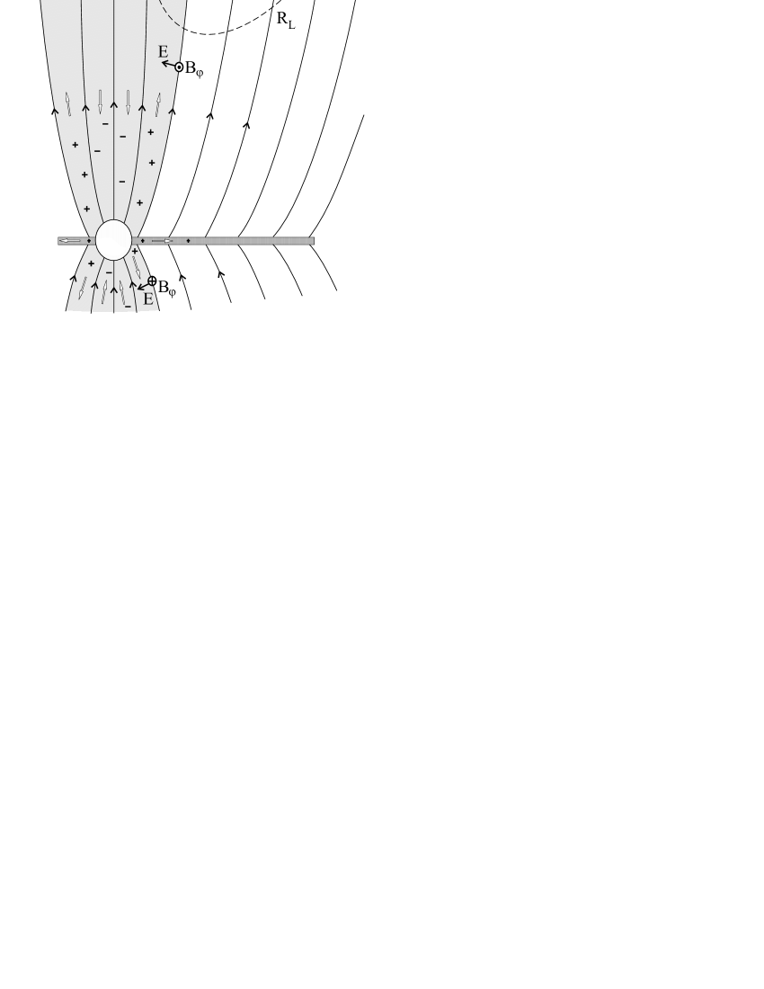
Figure 1: Blandford’s force-free paraboloidal solution. Here the thick arrows represent the volume currents. The shadowed region is the working volume $\Omega_{\rm F}\approx$ const. The dashed line represents the light cylinder.

We assume that in the vicinity of a central object the particle energy flux is much smaller than that of electro-magnetic field. In this case it is possible to consider the contribution of particle inertia as a small disturbance to the quantities of the force-free flow. Thus, in the first approximation we can get from (12) the linear equation on the disturbance and solve the problem self-consistently.

As was already stressed, for cold plasma the problem is characterized by two singular surfaces: Alfvénic and fast magnetosonic ones. Consequently, we need to specify four boundary conditions on the disc surface $D$ (Beskin, 1997). For simplicity, we consider the case

$$\Omega_{\rm F}(\Psi)|_{\rm D}=\mathrm{const}=\Omega_{\rm F},$$

$$\gamma|_{\rm D}=\mathrm{const}=\gamma_{\rm in}\ll\sigma^{1/3},$$

$$\eta(\Psi)|_{\rm D}=\mathrm{const}=\eta,$$

$$\Psi|_{\rm D}=\frac{\pi{\cal C}}{\Omega_{\rm F}}\mathrm{ln}\left(\Omega_{\rm F}\varpi+\sqrt{(\Omega_{\rm F}\varpi)^{2}+1}\right).$$

The condition $\Omega_{\rm F}=\mathrm{const}$ naturally restricts the region of a flow under consideration (see Fig. 1). Since we assume that the magnetic field is frozen in the disc, we must consider the flow only when $\Omega_{\rm F}X|_{D}=\Omega_{\rm F}\varpi<1$. In fact, we should use the inequality $\Omega_{\rm F}X\ll 1$. Then, Michel’s magnetization parameter $\sigma$ for our problem can be defined as

$$\sigma=\frac{E_{\rm A}}{\mu\eta}=\frac{{\cal C}\Omega_{\rm F}}{8\pi\mu\eta}.$$ (17)

Here $E_{\rm A}$ is a kind of energy amplitude:

$$E=\frac{{\cal C}\Omega_{\rm F}^{2}X}{4\pi\sqrt{1+\Omega_{\rm F}^{2}X^{2}}}\approx\frac{{\cal C}\Omega_{\rm F}^{2}X}{4\pi}=E_{\rm A}\cdot 2\Omega_{\rm F}X.$$ (18)

Under our assumptions $\sigma\gg 1$, and we can introduce the small quantity $\varepsilon=\sigma^{-1}$. Besides, we will be mainly interested in the flow far from the light cylinder, and so we have another limitation $\Omega_{\rm F}^{2}XY\gg 1$.

We shall seek the stream function of the problem in the form

$$\Psi(X,Y)=\Psi_{0}(X)+\varepsilon f(X,Y),$$ (19)

where $\varepsilon f(X,Y)$ is the disturbance to find. The function of the angular momentum $L$ may in general be different from the function $L_{0}$. For $L$ the following expression may be written:

$$L(\Psi)=L(\Psi_{0})+\varepsilon f\frac{\partial L(\Psi_{0})}{\partial\Psi_{0}}=L(\Psi_{0})+\varepsilon l.$$ (20)

4 Fast magnetosonic surface

In order to find the position of FMS one can rewrite the Bernoulli equation (11) in the form

$$\begin{array}[]{l}\displaystyle q^{4}+2q^{3}-\left(\xi+\frac{1}{\Omega_{\rm F}^{2}\varpi^{2}}\right)q^{2}+2q\left(\frac{\mu^{2}\eta^{2}}{E^{2}}+\frac{(e^{\prime})^{2}}{\Omega_{\rm F}\varpi^{2}}\right)+\\ \\ \displaystyle+\frac{\mu^{2}\eta^{2}}{E^{2}}+\frac{(e^{\prime})^{2}}{\Omega_{\rm F}\varpi^{2}}=0.\end{array}$$ (21)

Here by definition $q={\cal M}^{2}/\Omega_{\rm F}^{2}\varpi^{2}$,

$$\xi=1-\frac{\Omega_{\rm F}^{4}\varpi^{2}(\nabla\Psi)^{2}}{64\pi^{4}E^{2}},$$ (22)

and $e^{\prime}=E(\Psi)-\Omega_{\rm F}L(\Psi)=\mu\eta\gamma(1-\Omega_{\rm F}\varpi v_{\hat{\varphi}})\approx\gamma_{\rm in}\mu\eta=\mathrm{const}$. It is easy to check that for the force-free solution

$$\xi=\frac{1-\mathrm{cos}{\theta}}{2}\approx\frac{\theta^{2}}{4}\ll 1$$ (23)

for the small angle $\theta$, i.e., in the whole region near the rotational axis. Remember that $\xi\equiv 0$ for Michel force-free monopole outflow.

To show that the quantity $q$ is much smaller than unity, one can write (8) assuming $\sigma\gg 1$ and $\Omega_{\rm F}^{2}\varpi^{2}\gg 1$. Solving this equation for $q$, we get

$$q=\frac{\gamma\mu\eta}{E}\approx\frac{\gamma}{\sigma}.$$ (24)

Thus, $q$ is approximately equal to the ratio of particle kinetic energy to the full energy of the flow, i.e., $q\ll 1$ for the magnetically dominated flow.

As a result, one can rewrite (21) in the form

$$2q^{3}-\left(\xi+\frac{1}{\Omega_{\rm F}^{2}\varpi^{2}}\right)q^{2}+\frac{\mu^{2}\eta^{2}}{E^{2}}+\frac{(e^{\prime})^{2}}{\Omega_{\rm F}\varpi^{2}}=0,$$ (25)

where the terms $q^{4}$ and $q$ were omitted due to their smallness.

Fast magnetosonic surface corresponds to the intersection of two roots of equation (25), or to the condition of discriminant $Q$ being equal to zero (Beskin, Kuznetsova & Rafikov, 1998). The regularity conditions give $\partial Q/\partial r=0$ and $\partial Q/\partial\theta=0$, or $\partial Q/\partial X=0$ and $\partial Q/\partial Y=0$. For equation (25) discriminant $Q$ is expressed by

$$Q=\frac{1}{16}\frac{\mu^{4}\eta^{4}}{E^{4}}-\frac{1}{16}\frac{1}{27}\frac{\mu^{2}\eta^{2}}{E^{2}}\left(\xi+\frac{1}{\Omega_{\rm F}^{2}\varpi^{2}}\right)^{3}.$$ (26)

The condition of root intersection $Q=0$ can be rewritten as

$$\xi(r_{\rm F},\theta)+\frac{1}{\Omega_{\rm F}^{2}r_{\rm F}^{2}\theta^{2}}=3\left(\frac{\mu\eta}{E}\right)^{2/3},$$ (27)

and the first regularity condition $\partial Q/\partial Y$ as

$$Y\frac{\partial\xi}{\partial Y}=\frac{1}{\Omega_{\rm F}^{2}XY}.$$ (28)

Taking approximately $\xi\approx Y\cdot\partial\xi/\partial Y$ we get for the position of FMS

$$r_{\rm F}(\theta)\approx R_{\rm L}\left(\frac{\sigma}{\theta}\right)^{1/2},$$ (29)

where $R_{\rm L}=\Omega_{\rm F}^{-1}$ is the radius of a light cylinder.

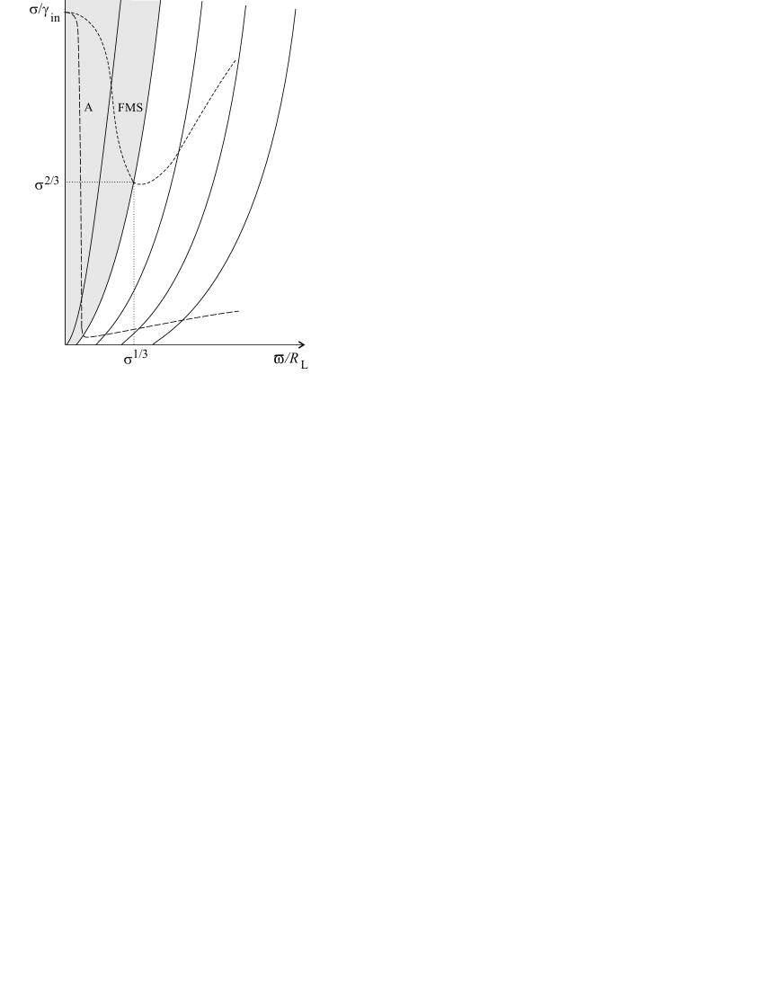
Figure 2: Position of the Alfvénic surface (long dashed line) and FMS (short dashed lines) for paraboloidal magnetic field. The self-similar flow can be realized only outside the working volume.

Values of $q(r_{\rm F},\theta)$ and $\gamma_{\rm F}=\gamma(r_{\rm F},\theta)$ due to condition $Q=0$ do not depend on the sum $(\xi+1/\Omega_{\rm F}^{2}\varpi^{2})$ and on the FMS are equal to

$$q(r_{\rm F},\theta)=\frac{1}{\sigma\theta},$$ (30)

$$\gamma_{\rm F}=(\sigma\theta)^{1/2}.$$ (31)

Again we confirm that $q\ll 1$ since $\sigma\theta=\Omega_{\rm F}^{2}XY|_{r_{\rm F}}\gg 1$. These results are valid when

$$\left(\frac{\mu\eta}{E}\right)^{2}\gg\left(\frac{e^{\prime}}{E\Omega_{\rm F}\varpi}\right)^{2},$$ (32)

i.e., in the region where electro-magnetic energy is greater than kinetic one. On the FMS this region is defined by the angle $\theta$ changing from $\gamma_{\rm in}^{2}\sigma^{-1}$ to $\sigma^{1/3}$. Here the greatest value of $\theta$ is given by the condition $\Omega_{\rm F}X=1$, which corresponds to the boundary of the working volume. On the other hand, for $\theta<\gamma_{\rm in}^{2}\sigma^{-1}$ one can get

$$r_{\rm F}\approx R_{\rm L}\frac{\sigma}{\gamma_{\rm in}},$$ (33)

$$\gamma_{\rm F}=\gamma_{\rm in}.$$ (34)

As we see, along the rotational axis particle energy remains the same as near the origin.

The position of the FMS on the rotational axis can be evaluated independently. Indeed, for $B_{\varphi}=0$ the condition $D=0$ coincides with the condition $A=0$, i.e., the position of the fast magnetosonic surface coincides with the Alfvénic surface on the axis. Assuming that $u_{\rm p}\approx\gamma_{\rm in}$ and using the definitions (4) and (17) one can obtain

$${\cal M}^{2}=\frac{\sigma}{\gamma_{\rm in}}\,\Omega_{\rm F}r.$$ (35)

It gives

$$r_{\rm F}\approx r_{\rm A}\approx\frac{\sigma}{\gamma_{\rm in}}R_{\rm L},$$ (36)

coinciding with (33). This distance is much larger than the appropriate radius $r_{\rm F}\approx(\sigma/\gamma_{\rm in})^{1/2}R_{\rm L}$ for monopole magnetic field. But the transverse dimension of the working volume $\varpi\approx\sigma^{1/3}R_{\rm L}$ remains the same. We see as well that on the FMS within the working volume the value of Lorentz factor changes from $\gamma_{\rm in}$ to $\sigma^{1/3}$. The greatest value of $\gamma$ is equal to the corresponding value for the monopole structure (Beskin, Kuznetsova & Rafikov, 1998).

Finally, as one can see in Fig. 2, the shape of the FMS extends along the rotational axis. Thus, the working volume cannot be described within the the self-similar approach as in this case the singular surfaces are to have conical shape $\theta=\mathrm{const}$ (Blanford & Payne, 1982; Li, Chiueh & Begelman, 1992).

5 Subsonic flow

For the inner region of the flow we shall write down the stream equation with the small disturbances to the functions $\Psi$, $L$, and $E$. We shall treat the quantities $q$ and $\varepsilon f$ as being of the same order of smallness. In the zero approximation one can get the equation

$$\begin{array}[]{l}\displaystyle-\frac{4\Omega_{\rm F}^{2}}{X+Y}\frac{\partial}{\partial X}\left(X\frac{\partial\Psi_{0}}{\partial X}\right)+\\ \\ \displaystyle+\frac{64\pi^{4}}{XY}\frac{1}{\partial\Psi_{0}/\partial X}L(\Psi_{0})\frac{\partial L(\Psi_{0})}{\partial X}=0.\end{array}$$ (37)

Clearly, it has a solution (16) for $L(\Psi_{0})=L_{0}(\Psi_{0})$. On the other hand, in the first approximation we have

$$\begin{array}[]{llll}\displaystyle-\frac{4\Omega_{\rm F}^{2}}{X+Y}\left[q\frac{\partial}{\partial X}\left(X\frac{\partial\Psi_{0}}{\partial X}\right)+X\frac{\partial q}{\partial X}\frac{\partial\Psi_{0}}{\partial X}\right]-\\ \\ \displaystyle-\frac{4\Omega_{\rm F}^{2}}{X+Y}\varepsilon\left(X\frac{\partial^{2}f}{\partial X^{2}}+\frac{\partial f}{\partial X}+Y\frac{\partial^{2}f}{\partial Y^{2}}+\frac{\partial f}{\partial Y}\right)+\\ \\ \displaystyle-\frac{1}{2}\cdot\frac{64\pi^{4}}{XY}q\frac{1}{\partial\Psi_{0}/\partial X}\frac{\partial L^{2}(\Psi_{0})}{\partial X}-\\ \\ \displaystyle+\frac{1}{2}\cdot\frac{64\pi^{4}}{XY}\varepsilon\frac{\partial f/\partial X}{(\partial\Psi_{0}/\partial X)^{2}}\frac{\partial L^{2}(\Psi_{0})}{\partial X}+\\ \\ \displaystyle+\frac{64\pi^{4}}{XY}\varepsilon\frac{1}{\partial\Psi_{0}/\partial X}\frac{\partial(L(\Psi_{0})l)}{\partial X}+\\ \\ \displaystyle+\frac{64\pi^{4}}{XY}\varepsilon\frac{e^{\prime}}{\Omega_{\rm F}}\frac{1}{\partial\Psi_{0}/\partial X}\frac{\partial L(\Psi_{0})}{\partial X}=0.\end{array}$$ (38)

The integral $L$ depends on the variable $Y$ as $\Psi=\Psi_{0}+\varepsilon f$ depends on it.

Before we proceed to solve equation (38) we can evaluate the ratio $\varepsilon f/\Psi_{0}$ on the fast magnetosonic surface. In order to do this, we need to express $\xi$ as a function of $\varepsilon f$:

$$\xi=\frac{2\varepsilon}{\pi{\cal C}}\left(\frac{f}{X}-\frac{\partial f}{\partial X}\right).$$ (39)

Given the order of $\xi$ on the FMS by (28), one can get

$$\frac{\varepsilon f}{\pi{\cal C}X}\sim\frac{1}{\Omega_{\rm F}^{2}XY}.$$ (40)

Thus,

$$\frac{\varepsilon f}{\Psi_{0}}\sim\frac{1}{\sigma\theta}\ll 1,$$ (41)

where $\sigma\theta\gg 1$ as we are interested in the flow structure outside the light cylinder. Hence, our disturbance proved to be small in comparison with the force-free solution up to the fast magnetosonic surface. Finally, from (38) we can get an equation on the function $\varepsilon f$:

$$\begin{array}[]{l}\displaystyle\varepsilon X^{2}\frac{\partial^{2}f}{\partial X^{2}}+\varepsilon X\frac{\partial f}{\partial X}-\varepsilon f+\varepsilon XY\frac{\partial^{2}f}{\partial Y^{2}}+\varepsilon X\frac{\partial f}{\partial Y}\\ \\ \displaystyle+\pi{\cal C}\left(2qX+X^{2}\frac{\partial q}{\partial X}\right)+\frac{4\pi^{2}e^{\prime}}{\Omega_{\rm F}^{2}}=0.\end{array}$$ (42)

To obtain $q$, we shall make a natural assumption that $q$ and $\xi$ grow monotonically from correspondingly $\sigma^{-1}$ and $0$ near the origin of the flow to $\left(\mu\eta/E\right)^{2/3}$ and $1/\Omega_{\rm F}^{2}\varpi^{2}$ on the fast magnetosonic surface. Thus, in (25) one can neglect the terms $q^{3}$ and $\xi q^{2}$ in comparison with $(\mu\eta/E)^{2}$ and $q^{2}/(\Omega_{\rm F}\varpi)^{2}$ correspondingly. After that the solution of (25) is expressed by

$$q=\frac{1}{2\sigma}\left(\frac{Y}{X}\right)^{1/2}.$$ (43)

It is necessary to stress that in equation (42) we can neglect the derivatives over $Y$ in comparison with the derivatives over $X$. Here we take into account our assumptions that $Y\gg X$, so that $\partial f/\partial X\sim f/X$ by the order of magnitude. Inside the working volume this means that we can neglect the curvature of field lines in our problem. Indeed, one can find that

$$k=\frac{1}{R_{\rm c}}=\frac{1}{Y}\left(\frac{X}{Y}\right)^{1/2}+\frac{2\varepsilon}{(XY)^{1/2}}\left(\frac{\partial f}{\partial Y}+Y\frac{\partial^{2}f}{\partial Y^{2}}\right),$$ (44)

formally writing the expression for curvature $k$ for the implicit function $\Psi_{0}(X(x,y))+\varepsilon f(X(x,y),Y(x,y))=\mathrm{const}$. Here the term $(X^{1/2}/Y^{3/2})$ corresponds to the inverse curvature radius of the force-free magnetic surfaces. Thus, the curvature term does not play any role in the force balance on the magnetic surfaces in the paraboloidal magnetic field, which was quite different for the monopole magnetic field. In the latter case the curvature term played the leading role in the asymptotic region (Beskin & Okamoto, 2000).

After substitution of the found function $q(X,Y)$ into (42), one can find for the disturbance of the stream function

$$\varepsilon f=\frac{\pi{\cal C}}{\sigma}\Omega_{\rm F}(XY)^{1/2},$$ (45)

with the Lorentz factor being equal to

$$\gamma=\Omega_{\rm F}(XY)^{1/2}=\Omega_{\rm F}r\sin\theta.$$ (46)

Thus, in the subsonic region the Lorentz factor grows linearly with the distance from the axis and reaches on the fast magnetosonic surface the value $(\sigma\theta)^{1/2}$, which corresponds to the result found in the previous Section. In this sense one can say that the solution in the inner region of the flow can be continued to the fast magnetosonic surface.

6 Supersonic flow

In order to solve the problem in the supersonic region we need to emphasize some features of the paraboloidal configuration of magnetic field.

1. The character of the flow may change in the vicinity of the singular surface.

2. It was shown above that for paraboloidal magnetic field the curvature of field lines does not play any role in the force balance inside the working volume $\Omega_{\rm F}X<1$. This allows us to consider the flow as one-dimensional.

3. Positions of the fast magnetosonic surfaces in the paraboloidal field and in the cylindrical field coincide.

Let us clarify the last point. The position of the fast magnetosonic surface for the magnetized cylindrical jet immersed into the external magnetic field $B_{\rm ext}$ is given by the relation (Beskin & Malyshkin, 2000)

$$\Omega_{\rm F}\varpi\sim\sigma\frac{B_{\rm ext}}{\Omega_{\rm F}^{2}\Psi_{\rm jet}},$$ (47)

where $\varpi\approx r\theta$ is the distance from the rotational axis, and $\Psi_{\rm jet}$ is the total flux inside the jet. On the other hand, according to our definition of $\sigma$ (17) for paraboloidal flow

$$E=2\mu\eta\sigma\Omega_{\rm F}X=\frac{\Omega_{\rm F}^{2}\Psi}{4\pi^{2}}.$$ (48)

As a result, we shall define the magnetic flux inside the region $\Omega_{\rm F}X<1$ as $\Psi_{\rm jet}$, and thus $\cal C$ is expressed by

$${\cal C}=\frac{\Psi_{\rm jet}\Omega_{\rm F}}{\pi}.$$ (49)

In this case the expressions for $\sigma$ for two flows coincide. Taking poloidal paraboloidal field as the external field for the one-dimensional flow

$$B_{\rm p}=\frac{{\cal C}}{2z},$$ (50)

one can get the position of the FMS

$$r_{\rm F}\sim R_{\rm L}\left(\frac{\sigma}{\theta}\right)^{1/2},$$ (51)

which coincides with (29).

Hence, the flow becomes actually 1D in the vicinity of the FMS, not to say about the supersonic region. For this reason we can consider the supersonic flow as one-dimensional. But unlike Beskin & Malyshkin (2000) we would use the paraboloidal magnetic field $B_{\rm p}(z)$ (50) outside the working volume as an external one. It gives us the slow $z$-dependence of all the values.

For the cylindrical flow the integrals of motion near the axis are the same as the integrals of motion in our paraboloidal problem:

$$L(\Psi)=\frac{\Omega_{\rm F}\Psi}{4\pi^{2}},$$ (52)

$$\Omega_{\rm F}(\Psi)=\mathrm{const},$$ (53)

$$\eta(\Psi)=\mathrm{const},$$ (54)

$$E(\Psi)=\gamma_{\rm in}\mu\eta+\Omega_{\rm F}L=e^{\prime}+\Omega_{\rm F}L,$$ (55)

where $e^{\prime}=\mathrm{const}$. Introducing non-dimensional variables

$$y=\sigma\frac{\Psi}{\Psi_{0}},$$ (56)

$$x=\Omega_{\rm F}\varpi,$$ (57)

one can rewrite equations (11)–(12) as a set of ordinary differential equations for $y$ and $M^{2}$ (Beskin & Malyshkin, 2000):

$$\begin{array}[]{l}\displaystyle(1-x^{2}-{\cal M}^{2})^{2}\left(\frac{dy}{dx}\right)^{2}=\frac{\gamma_{\rm in}^{2}x^{2}}{{\cal M}^{4}}(1-x^{2}-2{\cal M}^{2})+\\ \\ \displaystyle+x^{2}(\gamma_{\rm in}+2y)^{2}-4y^{2}-\frac{x^{2}}{{\cal M}^{4}}(1-x^{2}-{\cal M}^{2})^{2},\end{array}$$ (58)

$$\begin{array}[]{l}\displaystyle(\gamma_{\rm in}^{2}+x^{2}-1)\frac{d{\cal M}^{2}}{dx}=2x{\cal M}^{2}-\frac{\gamma_{\rm in}^{2}x{\cal M}^{2}}{(1-x^{2}-{\cal M}^{2})}+\\ \\ \displaystyle+\frac{4y^{2}{\cal M}^{6}}{x^{3}(1-x^{2}-{\cal M}^{2})}.\end{array}$$ (59)

We want to emphasize that in the work of Beskin & Malyshkin (2000) these differential equations were applicable only for the inner part of the jet, where the integrals of motion could be expressed as the linear functions of $\Psi$ and $\Omega_{\rm F}=\mathrm{const}$. In fact, in the case ${\cal M}^{2}\ll x^{2}$ (and that is in the range of parameters we are interested in) the solution for $B_{\rm p}$ is the same for an arbitrary function $\Omega_{\rm F}(\Psi)$: the equation (58) can be rewritten as (Beskin & Malyshkin, 2000)

$$B_{\rm z}(\varpi)=\frac{4\pi E(\Psi)}{\varpi^{2}\Omega_{\rm F}^{2}(\Psi)}.$$ (60)

As $E(\Psi)$ is proportional to the $\Omega_{\rm F}^{2}(\Psi)$, the particular expression for the angular velocity is not contained in the equation for $B_{\rm p}$. This ensures the continuity of the solution even in the region where the condition $\Omega_{\rm F}=\mathrm{const}$ does not hold.

Analytically, from the set of equations (58)–(59) one can get the following results:

1. $x\ll\gamma_{\rm in}$

   $${\cal M}^{2}={\cal M}_{0}^{2}=\mathrm{const},\;y=\frac{\gamma_{\rm in}}{2{\cal M}_{0}^{2}}x^{2},$$ (61)

   i.e., the poloidal magnetic field is approximately constant.

2. $x\gg\gamma_{\rm in}$

   1. ${\cal M}_{0}^{2}\gg\gamma_{\rm in}^{2}$

      $${\cal M}^{2}=\frac{{\cal M}_{0}^{2}}{\gamma_{\rm in}^{2}}x^{2},\;y\propto\mathrm{ln}{\frac{x}{\gamma_{\rm in}}},$$ (62)

      i.e., the poloidal magnetic field decreases as $B_{\rm p}\propto\varpi^{-2}$ (Chiueh, Li & Begelman, 1991; Eichler, 1993; Bogovalov, 1995).

   2. ${\cal M}_{0}^{2}\ll\gamma_{\rm in}^{2}$

      $${\cal M}^{2}=\frac{{\cal M}_{0}^{2}}{\gamma_{\rm in}}x,\;y=\frac{\gamma_{\rm in}}{2{\cal M}_{0}^{2}}x^{2},$$ (63)

      i.e., again $B_{\rm p}\approx$ const.

Using the connection $q=\gamma\mu\eta/E$, one gets for the Lorentz factor

$$\gamma=\frac{qE}{\mu\eta}=2{\cal M}^{2}\frac{y}{x^{2}}.$$ (64)

Then, for $x\gg\gamma_{\rm in}$ and ${\cal M}_{0}^{2}\ll\gamma_{\rm in}^{2}$ the following linear dependence is valid (Beskin & Malyshkin, 2000):

$$\gamma=x.$$ (65)

Let us find the distance along the axis until which the linear growth of the Lorentz factor continues. In order to do this one should write the constant poloidal magnetic field which defines ${\cal M}_{0}^{2}$:

$$B_{\rm z}=\frac{\Psi_{0}\Omega_{\rm F}^{2}}{2\pi\sigma x}\frac{dy}{dx}=\frac{\Psi_{0}\Omega_{\rm F}^{2}\gamma_{\rm in}}{2\pi\sigma{\cal M}_{0}^{2}}.$$ (66)

As this magnetic field should be equal to the outer one, we get

$$z=\sigma\gamma_{\rm in}R_{\rm L},$$ (67)

and the greatest Lorentz factor near the boundary of the working volume is

$$\gamma=(\sigma\gamma_{\rm in})^{1/2}.$$ (68)

For $z>\sigma\gamma_{\rm in}R_{\rm L}$ we shall perform numerical calculation in the intermediate region between two limits ${\cal M}_{0}\ll\gamma_{\rm in}$ and ${\cal M}_{0}\gg\gamma_{\rm in}$. The boundary condition is the equality of the magnetic flux and of magnetic field. Thus, for every $z$ we need to find the proper value of ${\cal M}_{0}^{2}$ that would allow us to make internal poloidal magnetic field on the border of the working volume be equal to the external paraboloidal magnetic filed, as the internal flux becomes equal to the total flux of a jet $\Psi_{\rm jet}$. In this case the border of the working volume $x_{\rm jet}$ is defined during the numerical integration. We expect it to be

$$x_{\rm jet}(z)=z^{1/2}.$$ (69)

The integration shows that it remains almost paraboloidal (see Fig. 3). Such an integration gives the linear growth of Lorentz factor until about $\sigma$ (see Fig. 4 and Appendix).

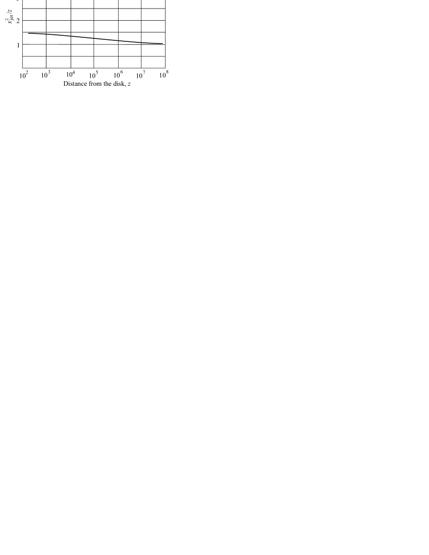
Figure 3: The border of the working volume $x_{\rm jet}$ as a function of $z$ for $\gamma_{\rm in}=8$ and $\sigma=10^{3}$. Its form remains almost paraboloidal. All the distances are given in the units of the light cylinder.

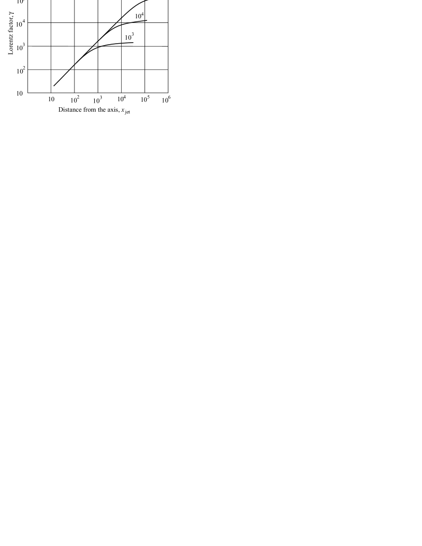
Figure 4: The growth of the Lorentz factor $\gamma$ near the border of the working volume as a function of the distance from the rotational axis (which is given in the units of the light cylinder) for different values of $\sigma$ ($10^{3}$, $10^{4}$, $10^{5}$) in a logarithmic scale. The linear growth of Lorentz factor continues until $\gamma\approx\sigma$.

Thus, the Lorentz factor $\gamma$ grows linearly with the distance from the axis reaching the value $\sigma$ near the border of the working volume for $z=\sigma^{2}R_{\rm L}$. This corresponds to the transformation of about a half of electro-magnetic energy into the kinetic one. The maximal Lorentz factor in this problem is $2\sigma$:

$$\frac{E}{\mu\eta}=\gamma_{\rm in}+2\sigma,$$ (70)

which follows from the definition (8). Thus, in the paraboloidal magnetic field the effective particle acceleration can be realized.

One can see that the condition for the particle acceleration from the work (Vlahakis, 2004)

$$\frac{\partial}{\partial\Psi}\left(\varpi^{2}B_{\rm P}\right)<0$$ (71)

holds for our geometry. Indeed, in our case this condition written for the border of the working volume $\Psi=\Psi_{\rm jet}$ transforms into the

$$\frac{\partial}{\partial\Psi}\left(\frac{x^{2}_{\rm jet}(z)}{z}\right)<0.$$ (72)

As the function $x^{2}_{\rm jet}(z)/z$ decreases along the field line (see Fig. 3), the condition (72) is fulfilled.

Here we should point out the main difference of our problem from the work in which the Michel’s monopole solution was taken as the first approximation.

1. Even the force-free flow is well collimated already.

2. The curvature term of the paraboloidal problem does not play any role in the force balance, which allowed us to treat the flow as one-dimensional in the supersonic domain.

3. The considered flow is supported from outside by the much greater flux than the one which is contained in the inner region. This allows the flow to widen and, consequently, to accelerate outflowing particles inside the working volume.

7 More realistic models

In the previous section we were discussing a model in which the rotational velocity $\Omega_{\rm F}$ of the field lines, which were assumed to penetrate a horizon of a black hole, in the working volume was constant, and it was equal to zero outside the working volume. This allowed us to regard the vacuum field outside the working volume as confining the flow. In this case the particle are accelerated effectively up to $\sigma$. However, such model does not seem to be realistic since we assume the non-rotating disk.

In this section we shall discuss two models. They would have three distinct regions. The first one is the working volume with the given law for rotational velocity, where we assume the MHD flow of the electron-positron plasma produced by the Blandford-Znajek process. The second one is the region of the, presumably, slow ion wind originating from the disk rotating with Keplerian velocity

$$\Omega_{\rm F}(y)=\Omega_{\rm F}(\sigma)\left(\frac{\sigma}{y}\right)^{3/2},$$ (73)

where we choose the parameters so that the function $\Omega_{\rm F}(y)$ would be continuous on the border of the working volume. The third region is the vacuum field where the disk angular velocity drops almost to zero. For our convenience we put $\Omega_{\rm F}$ being equal to zero at the distance where the Keplerian velocity drops ten times less than the rotational velocity near the axis. So we still have some portion of the vacuum magnetic flux to support our flow configuration.

The first model would be still characterized by $\Omega_{\rm F}=\mathrm{const}$ inside the working volume. For the second one we employ the following rotational velocity $\Omega_{\rm F}$, operating in the working volume:

$$\Omega_{\rm F}=\frac{(1-x^{2})[1+\mathrm{ln}(1+x)]}{\left\{4\mathrm{ln}{2}+1-x^{2}+[1-x^{2}-2(1+x)]\mathrm{ln}(1+x)\right\}}.$$ (74)

Here $x=\mathrm{cos}{\theta_{\rm H}}$, and $\theta_{\rm H}$ is the spherical angle at the horizon labeling the field line. It was first found in the work of Blanford & Znajek (1977) for the paraboloidal magnetic field threading the slowly rotating black hole. So the second model must be the most realistic.

For these two models we would perform the numerical calculation for the following set of the ordinal differential equations:

$$\begin{array}[]{l}\displaystyle A^{2}\left(\frac{dy}{dx}\right)^{2}=\frac{\gamma_{\rm in}^{2}x^{2}}{{\cal M}^{4}}(A-{\cal M}^{2})+\\ \\ \displaystyle+x^{2}\left(\gamma_{\rm in}+2\frac{\Omega_{\rm F}^{2}(y)}{\Omega_{\rm F}^{2}(0)}y\right)^{2}-4\frac{\Omega_{\rm F}^{2}(y)}{\Omega_{\rm F}^{2}(0)}y^{2}-\frac{x^{2}A^{2}}{{\cal M}^{4}},\end{array}$$ (75)

$$\begin{array}[]{l}\displaystyle\left(\gamma_{\rm in}^{2}+\frac{\Omega_{\rm F}^{2}(y)}{\Omega_{\rm F}^{2}(0)}x^{2}-1\right)\frac{d{\cal M}^{2}}{dx}=\frac{4y^{2}{\cal M}^{6}}{Ax^{3}}\frac{\Omega_{\rm F}^{2}(y)}{\Omega_{\rm F}^{2}(0)}-\\ \\ \displaystyle-\frac{x{\cal M}^{2}}{A}\frac{\Omega_{\rm F}^{2}(y)}{\Omega_{\rm F}^{2}(0)}(\gamma_{\rm in}^{2}-2A)+\frac{{\cal M}^{2}}{2}\frac{dy}{dx}\left(\frac{x^{2}}{\Omega_{\rm F}^{2}(0)}\frac{d\Omega_{\rm F}^{2}(y)}{dy}\right).\end{array}$$ (76)

The boundary condition again is the equality of the magnetic flux and of magnetic field at the border between the vacuum field and the internal flow with the variable rotational velocity $\Omega_{\rm F}$. We shall be interested in the characteristics of the flow in the working volume, assuming that the wind from the disk is governed by the MHD equations.

For the first model we see the same law for the particle Lorentz factor as a function of the $x$ on the border of the working volume as the one, we have gotten in the previous section. But now the border is compressed greater in comparison with its shape in the previous section (see Fig. 5), so the growth of the Lorentz factor along the axis is slightly slower.

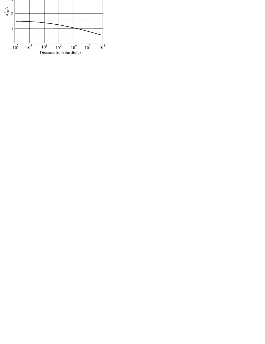
Figure 5: The border of the working volume $x_{\rm jet}$ as a function of $z$ for $\gamma_{\rm in}=8$ and $\sigma=10^{3}$. This curve is the same for both the first and the second models. Its form is only slightly compressed in comparison with parabola. All the distances are given in the units of the light cylinder.

The first question with the second model is whether the flow in subsonic region is greatly affected by the non-constant angular velocity of the field lines. It is easy to show, that the linearized equation (42) for the given function $\Omega_{\rm F}$ can be written as

$$\begin{array}[]{l}\displaystyle\varepsilon X^{2}\frac{\partial^{2}f}{\partial X^{2}}+\varepsilon X\frac{\partial f}{\partial X}\left(1+\frac{5}{2}M\right)-\varepsilon f+\varepsilon XY\frac{\partial^{2}f}{\partial Y^{2}}+\varepsilon X\frac{\partial f}{\partial Y}\\ \\ \displaystyle+\pi{\cal C}\left[2qX\left(1+\frac{1}{4}M\right)+X^{2}\frac{\partial q}{\partial X}\right]+\frac{4\pi^{2}e^{\prime}}{\Omega_{\rm F}^{2}}\left(1-\frac{1}{2}M\right)=0,\end{array}$$ (77)

where $\displaystyle M=\frac{\Psi}{\Omega_{\rm F}^{2}}\frac{d\Omega_{\rm F}^{2}}{d\Psi}$ is much smaller than the unity for $\Omega_{\rm F}X\ll 1$.

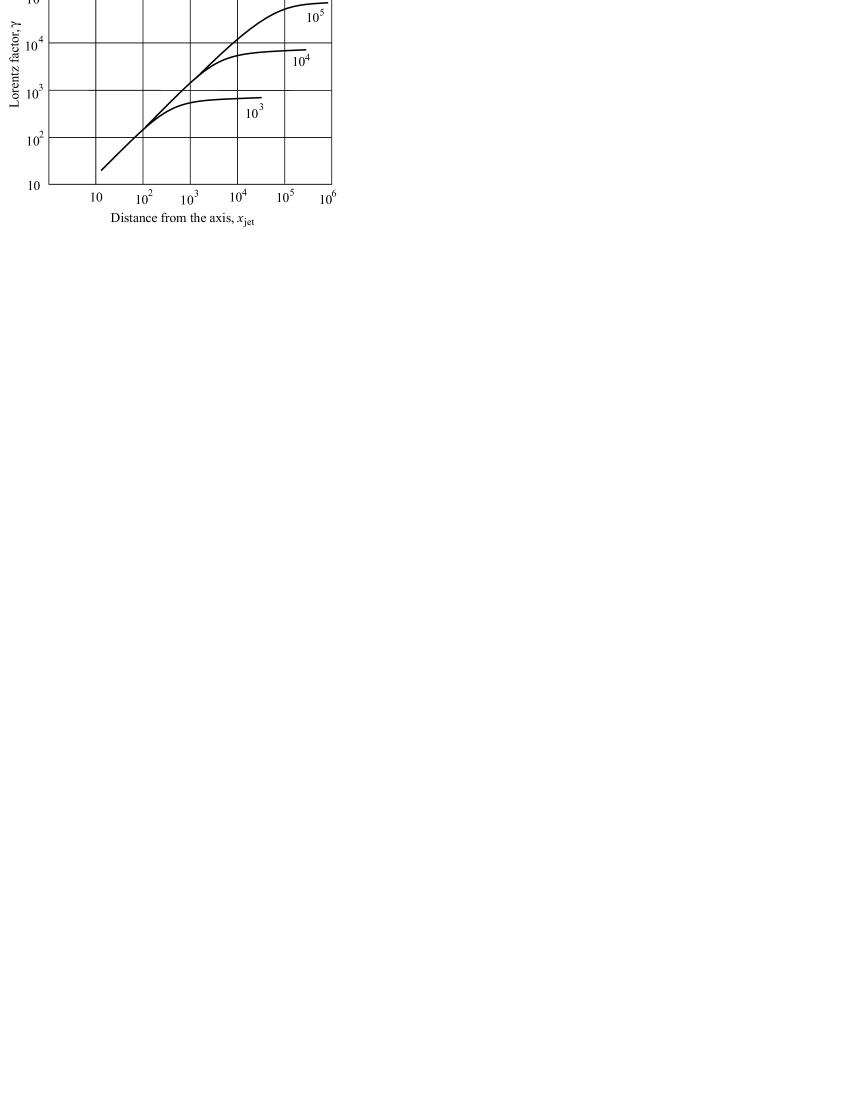
Figure 6: The growth of the Lorentz factor $\gamma$ near the border of the working volume as a function of the distance from the rotational axis (which is given in the units of the light cylinder) for different values of $\sigma$ ($10^{3}$, $10^{4}$, $10^{5}$) in a logarithmic scale is presented for the second model. Again the linear growth of Lorentz factor takes place, but it grows until approximately $0.5\sigma$.

The numerical integration shows again that the border of the working volume is compressed greater than it was for the vacuum field just outside the working volume. Besides, the growth of the Lorentz factor, although sustaining the shape of the previous curve $\mathrm{ln}{\gamma}(\mathrm{ln}{x})$, stops at smaller values than in the case of a constant rotational velocity (see Fig. 6). this results from the diminishing of the $\Omega_{\rm F}$ near the border of the working volume:

$$\gamma_{\rm max}=2\sigma\frac{\Omega_{\rm F}^{2}(\sigma)}{\Omega_{\rm F}^{2}(0)}.$$ (78)

As the $\Omega_{\rm F}^{2}(\sigma)/\Omega_{\rm F}^{2}(0)\approx 0.28$ for the Blandford-Znajek solution, so does the Lorentz factor at the border of the working volume. We may conclude that the decrease of the function $\Omega_{\rm F}$ generally suppresses the effectiveness of particle acceleration.

8 Discussion and Astrophysical Applications

In reality, there are at any way two reasons why the ideal picture under consideration may be destroyed. First of all, for large enough $\gamma$ the drag force $F_{\rm drag}\propto\gamma^{2}$ can be important. As was demonstrated in Beskin, Zakamska & Sol (2003), for monopole magnetic field it takes place when the compactness parameter $l_{\rm A}$ becomes larger than $\sigma^{1/3}$. Second, the particle acceleration continues only until the paraboloidal poloidal magnetic field can be realized. This can be stopped by the external magnetic field, say, by the galactic chaotic magnetic field $B_{\rm gal}\sim 10^{-6}$ G. The flow inside the border $\Omega_{\rm F}X=\mathrm{const}$ widens, while the external paraboloidal magnetic field $B_{\rm ext}$ is greater than the $B_{\rm gal}$. When they equate, the expansion stops and the particle acceleration ceases. The distance $x_{\rm st}$ from the axis at which $B_{\rm gal}=B_{\rm ext}$ is given by $x_{\rm st}^{2}=B_{0}/B_{\rm ext}$. Here $B_{0}=\Psi_{\rm jet}\Omega_{\rm F}^{2}$ is the magnetic field strength in the vicinity of the central object. Thus,

$$\gamma_{\rm max}=\mathrm{Min}\{x_{\rm st},\sigma\}.$$ (79)

The relation

$$\gamma\approx\left(\frac{B_{0}}{B_{\rm ext}}\right)^{1/2}$$ (80)

was already obtained in Beskin & Malyshkin (2000). As can be easily seen from (79), whether the Poynting flux will be transformed into the particle kinetic energy flux depends on the value of $\sigma$ and $B_{\rm ext}$.

We now consider several astrophysical applications.

8.1 Active Galactic Nuclei

For AGNs the central engine is assumed to be a rotating black hole with mass $M\sim 10^{9}M_{\odot}$, $R\sim 10^{14}$ cm, the total luminosity $L\sim 10^{45}$ erg s^-1, $B_{0}\sim 10^{4}$ G. In the Michel magnetization parameter $\sigma$ (1)

$$\sigma\approx 10^{14}\lambda^{-1}M_{9}B_{4}\left(\frac{\Omega R}{c}\right),$$ (81)

the main uncertainty comes from the multiplication parameter $\lambda$, i.e., in the particle number density $n$. Indeed, for an electron-positron outflow this value depends on the efficiency of pair creation in the magnetosphere of a black hole, which is still undetermined. In particular, this process depends on the density and energies of the photons in the immediate vicinity of the black hole. As a result, if the hard-photon density is not high, then the multiplication parameter is small ($\lambda\sim 10-100$; Beskin, Istomin & Pariev (1992); Hirotani & Okamoto (1998)). In this case for $(\Omega R/c)\sim 0.1$–$0.01$ we have $\sigma\sim 10^{9}-10^{12}$. Knowing $\sigma$ we can estimate the maximal Lorentz factor $\gamma_{\rm max}$ (79). In the presence of the external magnetic field of typical value $B_{\rm ext}=10^{-6}$G, $\gamma_{\rm max}=10^{5}\ll\sigma$, so only the small part of the Poynting flux can be transformed into the particle flux. On the other hand, if the density of photons with energies ${\cal E}_{\gamma}>1$MeV is high enough, direct particle creation $\gamma+\gamma\rightarrow e^{+}+e^{-}$ results in an increase of the particle density (Svensson, 1984). This gives $\sigma\sim 10-10^{3}$. In this case the Lorentz factor is $\gamma_{\rm max}=\sigma$, and the energy transformation can be efficient.

Recently the work of Gracia, Tsinganos, Bogovalov (2005) has been published in the electronic arXiv with an idea close to the one presented here (the central relativistic flow with the disk wind surrounding it), although with different formalization. In that work the comparison of the observational data for the jet opening angle with the model opening angle is presented. Here we can repeat the same for our paraboloidal inner flow. The distance for the angle range from the work of Biretta et al. (2002) lies well inside a sphere with the radius $z=R_{\rm L}\gamma_{\rm in}\sigma$, so we shall use the strictly paraboloidal form of the border of the working volume. We have one free parameter in this case: the value of $\Omega_{\rm F0}$ which we chose to be equal to $8.2\cdot 10^{-8}$. The result is presented in the Fig. 7. Although the analytical curve fails to explain the points at an angle $\approx 33$ degrees, it fits well the outer region and (surprisingly) the innermost point. The Lorentz factor for such distances is $\approx\gamma_{\rm in}$, so the jet possesses the same moderate Lorentz factor favoured in the works of Biretta et al. (1995), Biretta et al. (1999) and Cramphorn et al. (2004).

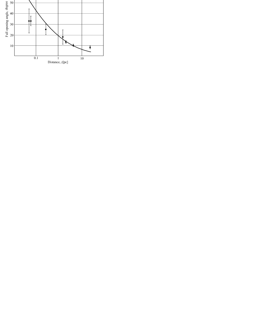
Figure 7: The observational data of the opening angle for M87 and the border of the working volume for $\Omega_{\rm F}(0)=8.2\cdot 10^{-8}\;s^{-1}$.

8.2 Radio Pulsars

For radio pulsars the central engine is a rotating neutron star with $M\sim M_{\odot}$, $R\sim 10^{6}$ cm, and $B_{0}\sim 10^{12}$ G. In this case the magnetization parameter $\sigma\sim 10^{4}$–$10^{6}$, corresponding to relativistic electron-positron plasma, is known with rather high accuracy (see, e.g., Bogovalov (1997)). The Lorentz factor in the presence of an external magnetic field is $\gamma_{\rm max}=10^{4}\sim\sigma$.

This estimate is valid, of course, only for the aligned rotator. In a case of an orthogonal rotator the situation with $\sigma$-problem is more explicit, as in this case the Goldriech-Julian charge density must be the $(\Omega R/c)^{1/2}$ smaller near the polar caps than that for the axisymmetric magnetosphere. Thus, it is natural to expect that the longitudinal current flowing along the open field lines would be proportionally smaller too (Beskin, Gurevich & Istomin, 1993). But, consequently, toroidal magnetic field will be smaller than the poloidal electric field in the vicinity of the light cylinder. On the other hand, it is known for the Michel’s monopole solution that in order to remove the light surface to infinity, the toroidal magnetic field must be of the same order as the poloidal electric field on the light cylinder. If the longitudinal current $j$ does not exceed by $(\Omega R/c)^{-1/2}$ times the quantity $\rho_{\rm GJ}^{90}c$, where $\rho_{\rm GJ}^{90}$ is an average charge density on the polar cap with $\chi\sim 90^{\circ}$ (for the typical pulsars this factor approach the value of $10^{2}$), the light surface for the orthogonal rotator must be located in the vicinity of the light cylinder. In this case the effective energy conversion and the current closure takes place in the boundary layer near the light surface (Beskin, Gurevich & Istomin, 1993; Chiueh, Li & Begelman, 1998; Beskin & Rafikov, 2000).

8.3 Cosmological Gamma-Ray Bursts

For cosmological gamma-ray bursts the central engine is represented by the merger of very rapidly orbiting neutron stars or black holes with $M\sim M_{\odot}$, $R\sim 10^{6}$ cm, and total luminosity $L\sim 10^{52}$ erg s^-1 (see, e.g., Lee at al (2000) for detail). On the other hand, even for a superstrong magnetic field of $B_{0}\sim 10^{15}$ G (which is necessary to explain the total energy release) the magnetization parameter $\sigma$ is small ($\sigma<1-100$), because within this model the magnetic field itself is secondary and its energy density cannot exceed the plasma energy density. Would it be not so, i.e., the magnetic field would be prior to the particle energy flow, we could formally apply our estimate. Having the external magnetic field to be the order of $10^{11}$ G, we can get the standard value for the Lorentz factor $\gamma_{\rm max}\sim 10^{2}$. However, in this case it is hard to explain of the value of $\sigma$ being the order of $10^{2}$.

9 Conclusion

We have gotten the characteristics of the flow in the paraboloidal magnetic field within the approach of stationary axisymmetric magnetohydrodynamics. To simplify the problem, we assumed that in the strongly magnetized flow with $\sigma\gg 1$ a particle inertia could be described as a small disturbance to the force-free flow. As the zero approximation the solution with paraboloidal magnetic field Blanford (1976) was taken.

The position of the fast magnetosonic surface is found to be $r_{\rm F}\approx(\sigma/\theta)^{1/2}R_{\rm L}$, with the Lorentz factor changing from $\gamma_{\rm in}$ to $\sigma^{1/3}$ on it. The disturbance $\varepsilon f$ to the stream function $\Psi$ is $\varepsilon f=\pi{\cal C}(\Omega_{F}^{2}XY)^{1/2}/\sigma\ll\Psi_{0}$ inside the FMS. As to the Lorentz factor $\gamma$, it grows linearly with the distance from the axis.

On the fast magnetosonic surface the structure of the flow may change significantly. It is implicitly confirmed by the fact that the characteristics of the flow, which we got under the assumption of the small disturbance in the supersonic region, is not in the agreement with the results on the FMS. However, in our problem the curvature term does not play role in the force balance on the magnetic surface, and the positions of the FMS in the cylindrical and paraboloidal flows coincide. These facts allowed us to regard the problem as one-dimensional and to perform numerical calculations.

As a result, we got the further growth $\gamma=(z/R_{\rm L})^{1/2}$ of the Lorentz factor until it reaches the value of $\sigma$ near the border of the working volume for $z\sim\sigma^{2}R_{\rm L}$ from the equatorial plane. This corresponds to almost the full conversion of the Poynting energy flux into the particle kinetic one.

For the more realistic model with three regions — the jet with the Blandford-Znajek rotational velocity, the disk wind, and the vacuum field — the particle acceleration is suppressed, but still the maximal Lorentz factor is of the order of $\sigma$.

We want to emphasize that our solution cannot be described in a self-similar way (Contopoulos, 1995; Vlahakis, 2004) as we assumed the constant angular velocity of the magnetic surfaces near the rotational axis. This structure cannot be considered within the self-similar approach.

Appendix A The analytical solution for the one-dimensional flow

Let us consider the set of equations (58)–(59). For $x\gg\gamma_{\rm in}$ and $y\gg\gamma_{\rm in}$ the system can be rewritten as

$$(x^{2}+{\cal M}^{2})^{2}\left(\frac{dy}{dx}\right)^{2}=4x^{2}y^{2},$$ (82)

$$x^{2}\frac{d{\cal M}^{2}}{dx}=2x{\cal M}^{2}+\frac{4y^{2}{\cal M}^{6}}{x^{3}(1-x^{2}-{\cal M}^{2})}.$$ (83)

Making the following substitutions

$$q=\frac{{\cal M}^{2}}{x^{2}},\;t=\frac{1}{x^{2}},\;z=y^{2},$$ (84)

and treating $z$ as a new variable, one can get the following set:

$$\frac{dq}{dz}=-tq^{3},$$ (85)

$$\frac{dt}{dz}=-\frac{t(1+q)}{2z}.$$ (86)

It is convenient to transform this set into the one second-order differential equation

$$\frac{d^{2}q}{dz^{2}}+\frac{1+q}{2z}\cdot\frac{dq}{dz}-\frac{3}{q}\cdot\left(\frac{dq}{dz}\right)^{2}=0.$$ (87)

Knowing its solution, one can get the function $t(z)$ as

$$t(z)=-\frac{dq/dz}{q^{3}}.$$ (88)

The solution of (87) gives

$$x=\frac{2a\sqrt{b(q-q_{1})(q-q_{2})}}{q}\left|\frac{q-q_{1}}{q-q_{2}}\right|^{1/\sqrt{1-b}},$$ (89)

$$y=\frac{ab(q-q_{1})(q-q_{2})}{q^{2}}\left|\frac{q-q_{1}}{q-q_{2}}\right|^{1/\sqrt{1-b}},$$ (90)

$$\gamma=\frac{\sqrt{b}}{2}\cdot\frac{\sqrt{(q-q_{1})(q-q_{2})}}{q+1}x.$$ (91)

Here

$$q_{1}=\frac{1-\sqrt{1-b}}{b},\;q_{2}=\frac{1+\sqrt{1-b}}{b},$$ (92)

$a$ and $b$ are constant, $0<a$, $-\infty<b<1$. For $b<0$ the maximal value of $q$ is equal to unity. On the other hand, for $b>0$ the value of $q$ is not limited. Thus, we would consider only the case $b>0$. For the ${\cal M}_{0}^{2}<\gamma_{\rm in}^{2}$ the solution is represented by the lower branch, and the case ${\cal M}_{0}^{2}>\gamma_{\rm in}^{2}$ by the upper branch of the graph (see Fig. A1).

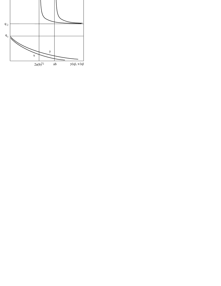
Figure 8: The functions x(q) and y(q).

Let us find the values of $a$ and $b$. In order to do this we shall regard two limits of this solution: for ${\cal M}_{0}^{2}\ll\gamma_{\rm in}^{2}$ and for ${\cal M}_{0}^{2}\gg\gamma_{\rm in}^{2}$. The condition ${\cal M}_{0}^{2}\ll\gamma_{\rm in}^{2}$ holds when $q\ll q_{1}<q_{2}$, so we get the known solution

$$y=Ax^{2}=\frac{1}{4a}\left(\frac{q_{2}}{q_{1}}\right)^{1/\sqrt{1-b}}x^{2},$$ (93)

$$q=\frac{B}{x}=2a\sqrt{bq_{1}q_{2}}\left(\frac{q_{1}}{q_{2}}\right)^{1/\sqrt{1-b}}\frac{1}{x}.$$ (94)

Equations $A=\gamma_{\rm in}/(2M_{0}^{2})$ and $B=M_{0}^{2}/\gamma_{\rm in}$ are not independent and give the following connection between $a$ and $b$:

$$a=\frac{{\cal M}_{0}^{2}}{2\gamma_{\rm in}}\left(\frac{1+\sqrt{1-b}}{1-\sqrt{1-b}}\right)^{1/\sqrt{1-b}}.$$ (95)

When $M_{0}^{2}\gg\gamma_{\rm in}^{2}$ $q=\mathrm{const}=M_{0}^{2}/\gamma_{\rm in}^{2}$, which corresponds to the asymptotical approach of $q$ to $q_{2}$. Thus, for $q_{2}=M_{0}^{2}/\gamma_{\rm in}^{2}$, one can get

$$b=\frac{2{\cal M}_{0}^{2}/\gamma_{\rm in}^{2}-1}{\left({\cal M}_{0}^{2}/\gamma_{\rm in}^{2}\right)^{2}}.$$ (96)

Thus,

$$a=\frac{{\cal M}_{0}^{2}}{2\gamma_{\rm in}}\left(2\frac{{\cal M}_{0}^{2}}{\gamma_{\rm in}^{2}}-1\right)^{\frac{{\cal M}_{0}^{2}/\gamma_{\rm in}^{2}}{{\cal M}_{0}^{2}/\gamma_{\rm in}^{2}-1}}.$$ (97)

Finally, for ${\cal M}_{0}^{2}\ll\gamma_{\rm in}^{2}$ (see the lower branch in the Fig. A1) the expressions (63) hold. In the intermediate region ${\cal M}_{0}^{2}\approx\gamma_{\rm in}^{2}$ (the upper branch in the Fig. A1) nothing can be said except the general formulas (89,90). For ${\cal M}_{0}^{2}\gg\gamma_{\rm in}^{2}$ (the upper branch in the Fig. A1, $q\rightarrow q_{2}$) we can get the refined expressions for $y(x)$ and ${\cal M}^{2}(x)$. Decomposing the functions (89)–(90) near $q_{2}$ as $q-q_{2}=\delta$, we get

$$x=C_{1}\delta^{(\sqrt{1-b}-2)/2\sqrt{1-b}},$$ (98)

$$y=C_{2}\delta^{(\sqrt{1-b}-1)/\sqrt{1-b}}.$$ (99)

Thus,

$$y=Ax^{2(\sqrt{1-b}-1)/(\sqrt{1-b}-2)}=Ax^{\frac{2}{1+M_{0}^{2}/\gamma_{\rm in}^{2}}},$$ (100)

where $A$ is constant. Thus, for $q=\mathrm{const}$ the expression for $y$ is not $\mathrm{ln}{x}$, but the exponential function of $x$ with the index depending on the quotient $M_{0}^{2}/\gamma_{\rm in}^{2}$, which changes from 1 to 0 (compare this result to the numerical calculation in Fig. 6). Lorentz factor is expressed in this case by (see Fig. 7)

$$\gamma\propto x^{\frac{2}{1+M_{0}^{2}/\gamma_{\rm in}^{2}}}.$$ (101)

So, if we assume that the effective grow of the Lorentz-factor continues until the exponent in (101) is equal to $1/2$, we can estimate the maximal Lorentz-factor by the value $\displaystyle\frac{3\sigma}{2}$ (compare it with the Fig. 4).

References

- Begelman, Blandford & Rees (1984) Begelman M.C., Blandford R.D., Rees M.J., 1984, Rev. Mod. Phys., 56, 255
- Begelman & Li (1994) Begelman M.C., Li Zh.-Yu., 1994, ApJ, 426, 269
- Beskin (1997) Beskin V.S., 1997, Phys. Uspekhi, 40, 659
- Beskin, Gurevich & Istomin (1993) Beskin V.S., Gurevich A.V., Istomin Ya.N., 1993, Physics of the pulsar magnetosphere, Cambridge University Press
- Beskin, Istomin & Pariev (1992) Beskin V.S., Istomin Ya.N., Pariev V.I., 1992, Sov. Astron., 36, 642
- Beskin, Kuznetsova & Rafikov (1998) Beskin V.S., Kuznetsova I.V., Rafikov R.R., 1998, MNRAS, 299, 341
- Beskin & Malyshkin (2000) Beskin V.S, Malyshkin L.M., 2000, Astron. Lett., 26, 208
- Beskin & Okamoto (2000) Beskin V.S, Okamoto I., 2000, MNRAS, 313, 445
- Beskin & Rafikov (2000) Beskin V.S., Rafikov R.R., 2000, MNRAS, 313, 433
- Beskin, Zakamska & Sol (2003) Beskin V.S., Zakamska N.L., Sol H., 2004, MNRAS, 347, 587
- Biretta et al. (1995) Biretta J.A., Zhou F., Owen F.N., 1995, ApJ, 447, 582
- Biretta et al. (1999) Biretta J.A., Sparks W.B., Macchetto F., 1999, ApJ, 520, 621
- Biretta et al. (2002) Biretta J.A., Junor W., Livio M., 2002, New Astronomy Review, 46, 239
- Blanford (1976) Blandford R.D., 1976, MNRAS, 176, 465
- Blanford & Payne (1982) Blandford R.D., Payne D.G., 1982. MNRAS, 199, 883
- Blanford & Znajek (1977) Blandford R.D., Znajek R.L., 1977, MNRAS, 179, 433
- Bogovalov (1995) Bogovalov S.V., 1995, Astron. Lett., 21, 565
- Bogovalov (1997) Bogovalov S.V., 1997, A&A, 327, 662
- Camenzind (1986) Camenzind M., 1986, A&A, 162, 32
- Chiueh, Li & Begelman (1991) Chiueh T., Li Zh.-Yu., Begelman M.C., 1991, ApJ, 377, 462
- Chiueh, Li & Begelman (1998) Chiueh T., Li Zh.-Yu., Begelman M.C., 1998, ApJ, 505, 835
- Contopoulos (1995) Contopoulos J., 1995, ApJ, 446, 67
- Coroniti (1990) Coroniti V.F., 1990, ApJ, 349, 538
- Cramphorn et al. (2004) Cramphorn C.K., Sazonov S.Y., Sunyaev R.A., 2004, A&A, 420, 33
- Eichler (1993) Eichler D., 1993, ApJ, 419, 111
- Gracia, Tsinganos, Bogovalov (2005) Gracia J., Tsinganos K., Bogovalov V., A&A accepted
- Hirotani & Okamoto (1998) Hirotani K., Okamoto I., 1998, ApJ, 497, 563
- Kennel & Coroniti (1984) Kennel C.F., Coroniti F.V., 1984, ApJ, 283, 694
- Kirk & Lyubarsky (2001) Kirk J.G., Lyubarsky Y., 2001, J. Astron. Soc. Australia, 18, 415
- Komissarov (2004) Komissarov S.S., 2004, MNRAS, 350, 1431
- Lee & Park (2004) Lee H.K., Park J., 2004, Phys.Rev.D, 70, 063001
- Lee at al (2000) Lee H.K., Wijers R.A.M.J., Brown G.E., 2000, Phys.Rep., 325, 83
- Li, Chiueh & Begelman (1992) Li Zh.-Yu., Chiueh T., Begelman M.C., 1992, ApJ, 394, 459
- Lyubarsky & Kirk (2001) Lyubarsky Y., Kirk J.G., 2001, ApJ, 547, 437
- Michel (1969) Michel F. C., 1969, Astrophys. J., 158, 727
- Michel (1991) Michel F., 1991, Theory of neutron star magnetosphere, Chicago University Press
- Sikora et al (2005) Sikora M., Begelman M.C., Madejski G.M., Lasota J.-P., astro-ph/0502115
- Spitkovsky & Arons (2004) Spitkovsky A., Arons J., 2004, ApJ, 603, 669
- Svensson (1984) Svensson R., 1984, MNRAS, 209, 175
- Thomson, Chang, & Quataert (2004) Thomson T.A., Chang P., Quataert E., 2004, ApJ, 611, 380
- Vlahakis (2004) Vlahakis N., 2004, ApJ, 600, 324