On the shape of the UHE cosmic ray spectrum

Abstract

We fit the ultra high energy cosmic ray spectra above $10^{19}\,\mathrm{eV}$ with different injection spectra at cosmic ray sources that are uniformly and homogeneously distributed in the Universe. We conclude that the current UHE spectra are consistent with power laws of index $\alpha$ between 2.4 and 2.7. There is a slow dependence of these indices on the cosmological evolution of the cosmic ray sources, which in this model determines the end of the galactic cosmic rays spectrum.

I Introduction

The current results on the energy spectrum of the highest energy cosmic rays are not fully consistent. The two high statistics experiments, AGASA AGASA and HiRes HiRes_PRL , do not agree on the normalization of the ultra high energy cosmic ray (UHECR) spectrum. In addition, HiRes results are consistent with a GZK GZK suppression, and AGASA claims a spectrum extended to higher energy. With the current statistics the differences are not very significant – the number of events above $10^{20}\,\mathrm{eV}$ differs by less than 3$\sigma$ BDMO . The normalizations of the spectra are quite different, especially in the common $E^{3}\times\mathrm{d}N/\mathrm{d}E$ presentation, but a renormalization of the energy assignment by 15–20%, which is within the reported systematic uncertainty of the energy assignment, of both data sets leads to a good agreement BDMO ; TSRiken . The high energy extension and exact normalization of the UHECR spectrum are thus not well known, but after the renormalization both experiments show the same spectral shape between $10^{18.5}$ and $10^{20}\,\mathrm{eV}$.

There have been recently several attempts BGG1 ; WB ; WW ; BGG2 ; L04 ; AB04 ; HiRes_APP ; SS05 to explain this shape with different injection spectra of extragalactic protons after propagation to the observer from isotropically and homogeneously distributed sources. The assumed injection spectra and to certain extent the cosmological evolution of the sources determine the shape of the extragalactic cosmic ray spectrum at Earth. A subtraction from the observed cosmic ray spectrum in these models determines also the end of the galactic cosmic ray spectrum. There are two types of solutions. Flat injection spectra, $\mathrm{d}N/\mathrm{d}E=AE^{-2}$, are suggested in Refs. WB ; WW . In this case the galactic cosmic rays spectrum extends above $10^{19}\,\mathrm{eV}$. The other popular solution is to use much steeper injection spectra with spectral indices $\alpha$ = 2.6–2.7. Such solutions set the end of the galactic cosmic ray spectrum at lower energy. The assumption that the extragalactic cosmic rays have a large fraction of nuclei heavier than Hydrogen APKGO05 modifies the propagation process and can potentially initiate a new class of models, in which the composition at injection introduces more model parameters.

Cosmic ray data is not yet good enough to prove that any of these models are correct. Fitting the spectra with several different parameters and the uncertain knowledge of the cosmic ray composition at $10^{19}\,\mathrm{eV}$ makes all models plausible.

We describe an attempt to fit the renormalized AGASA and HiRes spectra with injection spectra and cosmological evolution parameters covering practically the whole phase space and to use the quality of the fits as a measure of the plausibility of the models. This involves several assumptions that, although used in many previous publications, may not be correct. The main one is that extragalactic cosmic rays are protons and that the renormalized experimental spectra represent correctly the shape of the UHECR spectrum. One of the fit parameters is the required extragalactic cosmic ray luminosity at present time. The uncertainty of the luminosity depends on the arbitrary renormalization of the experimental data, as well on the cross correlation with other parameters and assumptions.

This paper is organized as follows: Section 2 describes the fitting procedures that we use, Section 3 gives the main results of the fits, and Section 4 discusses the results, compares to other fits and derives the main conclusions from this research.

II Fitting the UHECR spectrum

It was shown in Refs. BDMO ; TSRiken that a renormalization of about 15% of the energy assignment of the AGASA and HiRes events, would bring the two spectra in very good agreement in the energy region below $10^{20}\,\mathrm{eV}$ in both normalization and shape. In Ref. BDMO it was also shown that the statistics of events above $10^{20}\,\mathrm{eV}$ is too small to achieve a conclusive result about the end of the UHECR spectrum. In this paper we study how the best fit to the injection spectrum depends on the source parameters: injection spectrum, luminosity and luminosity evolution with redshift. To do so, supported by the above-mentioned findings, we fit these injection parameters to the energy-shifted spectra in the energy range $10^{19}$–$10^{20}\,\mathrm{eV}$. We chose as lower bound $10^{19}\,\mathrm{eV}$ because we expect at this energy the particles to be mostly extra-galactic and $10^{20}\,\mathrm{eV}$ as higher bound because of the sparseness of data above this threshold.

To calculate the expected spectrum from a isotropic homogeneous distribution of proton sources we use the analytical approach presented in Ref. bg ; BGG1 . In this approach all proton energy losses are included (redshift losses, pair and pion production losses) and they are all treated as continuous. This is the correct treatment for redshift losses and it is well suited for pair production and for pion production at large propagation distances. At small propagation distance, however, the large inelasticity of the pion production process produces large fluctuations in the expected fluxes that cannot be reproduced in the continuous energy loss approximation. A Monte Carlo simulation is better suited in this case. In the present paper, since pion production affects mostly the highest part of the energy spectrum, and we are only interested in the spectra below $10^{20}\,\mathrm{eV}$, we can safely use the continuous energy loss approximation for all energy loss processes.

Figure 1: Solid line: loss length for photo-pion and photo-pair production for protons as calculated in Ref. BGG1 . The dashed lines report the separate contribution of the two processes. The dotted line shows the loss length for redshift losses. The squares represent the loss length of Ref. Stanev:2000fb .

We assume the sources inject protons with a power-law spectrum, $E^{-\alpha}$, with a sharp cutoff at $E_{\mathrm{max}}=10^{21.5}\,\mathrm{eV}$. Changing the value of $E_{\mathrm{max}}$ does not appreciably affect the results in the energy region we are interested in. We assume the source emissivity to evolve as $L(z)=L_{0}(1+z)^{m}$, where $L_{0}$ is the present cosmic ray emissivity of the sources and $m=0$ corresponds to absence of evolution. There is no cutoff to the evolution of the luminosity because we are only interested in the region above $10^{18.5}\,\mathrm{eV}$ and in this region the contributions to the observed flux can come only from sources with $z\lesssim 0.5$. To calculate the energy losses we use the loss-lengths of Ref. BGG1 , plotted in Fig. 1, that were shown to be indistinguishable from the ones of Ref. Stanev:2000fb in the low energy region and within 15% at high energy BGG1 . We assume a $\Lambda$CDM universe with $\Omega_{\Lambda}=0.7$, $\Omega_{m}=0.3$ and $H_{0}=75\,\mathrm{km}\,\mathrm{s}^{-1}\,\mathrm{Mpc}^{-1}$.

We explore the parameter region in $\alpha$ from 2.05 to 3.00 in steps of 0.05 and in $m$ from 0 to 4 in steps of 0.25. For each $(\alpha,m)$ pair we calculate the expected flux and then the best fit emissivity, $L_{0}$, minimizing the $\chi^{2}$ indicator. To emulate the experimental energy resolution we include 30% Gaussian error distribution in the spectra after propagation. The effect of the energy resolution is to smooth the features produced by the propagation on the photon background and to lessen the GZK suppression BDMO .

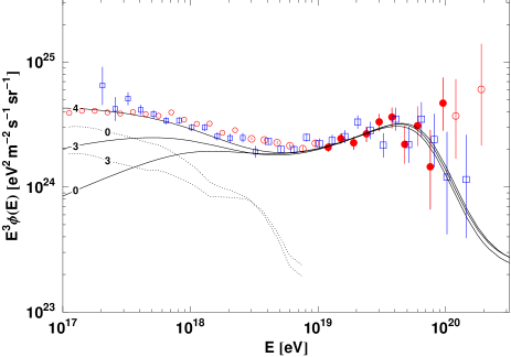
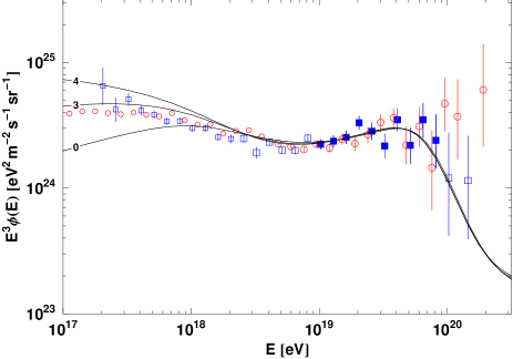
Figure 2: Upper panel: Best fits to the AGASA $-15\%$ dataset in the $10^{19}$–$10^{20}\,\mathrm{eV}$ energy range. Squares with error bars: HiRes dataset. Circles with error bars: AGASA&Akeno dataset. Filled symbols: points used in the fit. Smaller data points: data from HiRes2 and from Akeno (not shifted) to show the low-energy shape of the spectrum. Solid lines: best fits for different values of $m$. Dotted lines: galactic component needed in order to fit the spectrum at lower energy. The numbers attached to the lines indicate the value of $m$. Lower panel: best fit for the HiRes $+15\%$ dataset.

For AGASA and Akeno we use the data from Ref. AGASA , whereas for HiRes 1&2 we use the data from their website HiResweb which is very close to the published results HiRes_PRL ; HiRes_APP . Following the suggestion of Ref. BDMO we shift the AGASA and HiRes energies respectively by $-15\%$ and $+15\%$, while we leave the Akeno energies unchanged NaganoWatson . To do the shift we proceed in the following way: we calculate $\frac{\mathrm{d}N}{\mathrm{d}\log_{10}(E)}(E)$ and we assign this flux, calculated in $E$, to the energy $kE$. This means that: $\left(\frac{\mathrm{d}N}{\mathrm{d}E}(kE)\right)^{\mathrm{new}}=\frac{1}{k}\left(\frac{\mathrm{d}N}{\mathrm{d}E}(E)\right)^{\mathrm{old}}$ or $\left(k^{3}E^{3}\frac{\mathrm{d}N}{\mathrm{d}E}(kE)\right)^{\mathrm{new}}=k^{2}\left(E^{3}\frac{\mathrm{d}N}{\mathrm{d}E}(E)\right)^{\mathrm{old}}$, where $k=1.15$ for HiRes 1&2 and $k=0.85$ for AGASA. These new, shifted, datasets agree quite well almost over the whole energy range as shown in Fig. 2.

III Results from the fits

We applied the method presented in the previous paragraph to the AGASA $-15\%$ data fitting the points in the energy range $10^{19}$–$10^{20}\,\mathrm{eV}$. The results are shown in the upper panel of Fig. 2 where we plot the best fits for $m=0,3,4$ (solid lines). We only show results for $m$ = 3 and 4 because these values bracket the cosmological evolution derived from star forming regions and from gamma ray bursts. The corresponding slopes are, respectively, $\alpha=2.55,2.45,2.45$ with 1$\sigma$ errors of about 0.20. As it is clear from the plot all the three curves fit well the data in the region considered, with different degrees of goodness at low energy. The dotted lines represent the needed galactic component to fit the spectrum. The best fit with $m$=4 does not allow for galactic component above $10^{17}\,\mathrm{eV}$.

We repeated the same exercise for the HiRes $+15\%$ dataset (which is shown in the lower panel of Fig. 2) and the results were similar. The slopes are somewhat steeper, by about 0.05–0.1, well within the similarly large uncertainties. The main difference is at energies much lower than the fitting range, where the fits of the HiRes data set do not allow for a galactic component in cases with cosmological evolution. The flux of extragalactic cosmic rays below $10^{19}\,\mathrm{eV}$ has to be slightly decreased by some additional process in order not to exceed the Akeno and HiRes measurements. The shape of the spectra in the considered region is, however, the same for both experiments.

It has to be noted that the inclusion of the error distribution in the fit affects the spectral shape - the pile-up approaching $10^{20}\,\mathrm{eV}$ is visibly smoother. Since the points immediately above $10^{19}\,\mathrm{eV}$ have the lowest error bars, and thus affect the fit the most, the slope of the spectrum is increased by at most 0.05, much smaller than the uncertainties from the fits.

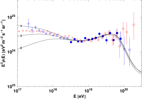
Figure 3: Best fits to the HiRes $+15\%$ dataset in the $10^{18.5}$–$10^{20}\,\mathrm{eV}$ energy range. Symbols are the same as in Fig. 2.

The best fitting parameters depend slowly on the fitted energy range. Fig. 3 shows the fit of the HiRes $+15\%$ data set for the energy range between $10^{18.5}$-$10^{20}\,\mathrm{eV}$ range. The best fit with $m$=4 again does not leave space for a galactic component below $10^{18}\,\mathrm{eV}$. The best spectral indices are 2.6, 2.5, and 2.5 respectively for $m$ = 0, 3, and 4, slightly smaller than those for the higher fitting threshold and almost identical to the AGASA $-15\%$ set shown in Fig. 2. The 1$\sigma$ error bars decrease to about $\pm$0.1. The effect of the wider fitting range on the AGASA $-15\%$ spectrum is similarly small, although for this data set it increases the spectral slopes for all $m$ values by 0.05–0.1. The 1$\sigma$ fit errors decrease to slightly less than $\pm$0.1.

As a consistency check we also fitted the unmodified AGASA and HiRes spectra. The results we obtain are much like the ones presented above. The best fit parameters differ by about 0.05–0.1, with the same $\pm$0.2 errorbars.

We performed several other fits varying the fitting threshold between $10^{18.5}$ and $10^{19.2}\,\mathrm{eV}$ and convinced ourselves that all fits returned consistent results within the 1$\sigma$ errors of the presented fits as shown in Fig. 4.

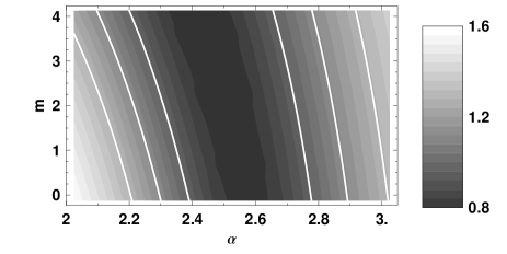
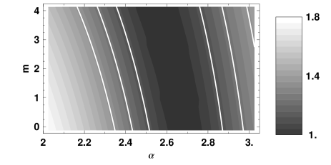
Figure 4: Contour plots of $\log_{10}\chi^{2}$ as a function of $\alpha$ and $m$ for the AGASA $-15\%$ dataset (upper panel) and for the HiRes $+15\%$ data set (lower panel) fits above 10¹⁹ eV. The white lines are the contours corresponding to $1\sigma$, $2\sigma$ and $3\sigma$.

In this figure we plot in the top panel $\log_{10}\chi^{2}$ as a function of $(\alpha,m)$ for the AGASA $-15\%$ fit above $10^{19}\,\mathrm{eV}$, i.e. for six degrees of freedom. The analogous fitting of the HiRes $+15\%$ set is shown in the bottom panel. The white contours are the confidence bands for $1\sigma$, $2\sigma$ and $3\sigma$. All $m$ values can provide a good fit to the data as the best fit $\alpha$ value slowly decreases with increasing $m$. This correlation is easily understood as with a smaller value of $\alpha$ less low energy particles are injected and to compensate for that one needs a stronger evolution of the sources to increase the number of low energy particles reaching the observer. For the HiRes $+15\%$ dataset the best fit parameters are in the strip connecting $(\alpha=2.6,m=0)$ and $(\alpha=2.4,m=4)$. As it is clear from the confidence bands in the plot, the present data sets do not restrict very much the values of the parameters, $\alpha$ being determined with an uncertainty of $\pm 0.2$ for a given $m$ and $m$ being almost free for a given $\alpha$. It is obvious, though, that fits with a flat injection spectrum do not give good $\chi^{2}$ values even with a strong cosmological evolution. Injection spectrum with $\alpha=2.0$ would be in the 3$\sigma$ range only in the case of $m=4$. Flat injection spectrum models require that the galactic cosmic ray spectrum extends to $10^{19.5}\,\mathrm{eV}$.

If the shape of the cosmic ray spectrum is the same as the one derived from the existing experimental statistics, even much higher future statistics from the Auger observatory Auger would not help to solve it. We performed a fit with the current spectral shape and increased statistics that corresponds to the one expected from Auger. The 1$\sigma$ errors on $\alpha$ for the fits above $10^{19}\,\mathrm{eV}$ became only slightly narrower $\pm$0.15. The measurement of the cosmic ray chemical composition, or, a measurement of the flux of cosmogenic neutrinos generated by UHECR in propagation to us ss05 , are needed to disentangle the two parameters.

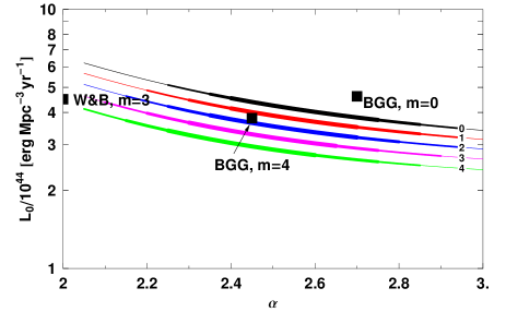
Figure 5: Required emissivity as a function of $(\alpha,m)$. Lines: best fit emissivity (above $10^{19}\,\mathrm{eV}$) as a function of $\alpha$. The numbers attached to the lines give the value of $m$. Every line is highlighted with different thicknesses corresponding to the confidence bands for $1\sigma$, $2\sigma$ and $3\sigma$. The black squares are the best fits obtained in other works. W&B corresponds to Ref. WB ; W95 , BGG corresponds to Ref. BGG1 .

In Fig. 5 we plot the best fit present day emissivities above $10^{19}\,\mathrm{eV}$ as a function of $\alpha$ for different values of $m$. In this plot we also show the values obtained in Ref. BGG1 ; WB ; W95 . The differences with the results of Ref. BGG1 are likely due to the slightly different dataset, to the different range of data used for the fits and to the inclusion in our calculation of the experimental energy resolution. There is also a factor because the fits were performed with a $-10\%$ shift of the AGASA data set instead of the $-15\%$ shift used here. It is interesting to note that the required values of the emissivity above $10^{19}\,\mathrm{eV}$ cover a narrow range between 2 and $6\cdot 10^{44}\,\mathrm{erg}\,\mathrm{Mpc}^{-3}\,\mathrm{yr}^{-1}$ and that the required luminosity increases with the flattening of the injection spectrum. This is a consequence of the fact that we only present the luminosity required above $10^{19}\,\mathrm{eV}$. If we were to extend the energy spectrum to lower energy, say to $10^{17}\,\mathrm{eV}$, we would observe exactly the opposite trend - steeper injection spectra would require much higher luminosity than flatter ones.

IV Discussion and conclusions

After fitting the shifted AGASA and HiRes data sets in terms of injection spectral index and cosmological evolution of the cosmic ray sources for an isotropic and homogeneous source distribution we obtained current emissivities above $10^{19}\,\mathrm{eV}$ that differ only by about a factor of two. In this sense we confirm the statement of Waxman W95 that approximately the same emissivity is required for a wide range on injection spectral indices. We disagree with the estimate of the central spectral index in Ref. W95 and find a significantly steeper one.

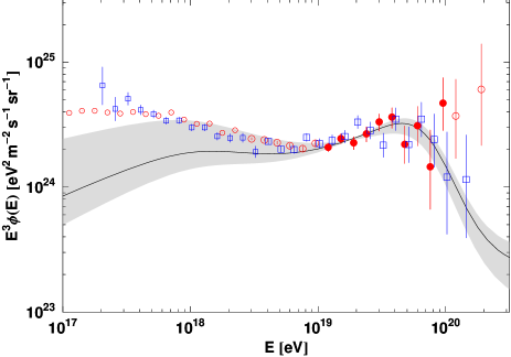
Figure 6: One $\sigma$ error band (shaded) of the AGASA fit with $m$=0 above 10¹⁹ eV.

Best fit spectral indices are, however, not well restricted by current statistics. In Fig. 6 we show with shaded area the 1$\sigma$ errors of the best fit prediction from the AGASA data above $10^{19}\,\mathrm{eV}$ (top panel of Fig. 2) for $m$ = 0. The figure emphasizes the perils of all fits of the extragalactic cosmic ray component with the current statistics. Such fits are most sensitive to, and attracted by, a small number of experimental points with the best statistics, in our case four points between $10^{19}$ and $10^{19.4}\,\mathrm{eV}$. Fitting uncertainties do not affect much the higher energy spectra where the GZK suppression prevails almost independently of the injection spectral index but create a large uncertainty below $10^{18.5}\,\mathrm{eV}$. This uncertainty makes estimates of the end of the galactic cosmic ray spectrum by subtraction of the model predictions from the total observed flux unreliable.

The luminosities that we show in Fig. 5 apply only to energies above $10^{19}\,\mathrm{eV}$. If one is interested in the total cosmic ray luminosity of the cosmic ray sources one should continue the integration to much lower energies. This introduces several possible new astrophysical parameters that come from the exact acceleration mechanism of the extragalactic cosmic rays. One could integrate down to the proton mass and obtain the highest possible emissivity. On the other hand studies of particle acceleration at relativistic shocks Achtetal find a minimum acceleration energy of $m\Gamma_{\rm shock}^{2}$ which for $\Gamma_{\rm shock}$ = 1000, as in gamma ray bursts, could be $10^{15}\,\mathrm{eV}$ and would decrease significantly the required emissivity. Modifications of the cosmic ray spectrum on propagation, such as suggested in Refs. L04 ; AB04 ; parizot04 because of magnetic horizon of the high energy cosmic rays Stanev:2000fb would not change the required emissivity. Such modifications would however change very much the extra-galactic cosmic ray spectrum suppressing the flux at the lower energy end and by consequence changing the shape of the end of the galactic cosmic ray spectrum required in order to fit the observations.

Fits of the monocular HiRes data have been performed by the HiRes group Bergman_fit . The best fit is obtained for $\alpha$ = 2.38$\pm$0.04 and $m$ = 2.8$\pm$0.3 for a total of 42 data points above $10^{17}\,\mathrm{eV}$ and respectively 39 degrees of freedom. In additon to the different energy range of the fit, HiRes assumes a ‘toy’ galactic cosmic ray model based on their composition measurement HiRes_comp that suggests domination of the extragalactic cosmic rays above 10¹⁸ eV.

The HiRes fit is probably dominated by lower energy cosmic rays ($10^{17.5-18.5}\,\mathrm{eV}$) with much smaller error bars. The two fits give different central values for $\alpha$ and $m$ but they are qualitatively consistent in the conclusion that even with a strong cosmological evolution of the cosmic ray sources the observed spectra do not support flat injection spectra.

We have fitted the shape of the ultrahigh energy cosmic ray spectrum above $10^{19}\,\mathrm{eV}$ assuming that these cosmic rays are protons, and that the sources of these protons are uniformly and homogeneously distributed in the Universe. The fits of the scaled AGASA and HiRes data sets allow for power law injection spectra in the range $AE^{-(2.4-2.7)}$ for cosmological evolution of the cosmic ray sources between $(1+z)^{4}$ to $(1+z)^{0}$. The cosmic ray emissivities above $10^{19}\,\mathrm{eV}$ required by different models are within about a factor of two in this range. The best fit spectral index decreases for strong evolution models. Flatter injection spectra do not fit well the cosmic ray spectra above $10^{19}\,\mathrm{eV}$. This also means that the end of the galactic cosmic ray spectrum is at, or below, $10^{18}\,\mathrm{eV}$ depending on the cosmological evolution of the extragalactic cosmic ray sources. Consistent data on the cosmic ray composition in the energy range above $10^{17}\,\mathrm{eV}$ are required in order to reveal the end of the galactic cosmic ray spectrum and thus help determine that of the extragalactic sources.

Acknowledgments. We thank D. Seckel for useful discussions. This research is funded in part by NASA APT grant NNG04GK86G.

References

- (1) M. Takeda et al.(AGASA Collaboration), Phys.Rev.Lett. 81:1163, (1998);M. Takeda et al. (AGASA Collaboration), Astropart. Phys. 19, 447 (2003), see also the AGASA web page http://www-akeno.icrr.u-tokyo.ac.jp/AGASA.
- (2) R.U. Abbasi et al. (HiRes Collaboration) Phys.Rev.Lett. 92:151101 (2004)
- (3) K. Greisen, Phys. Rev. Lett. 16, 748 (1966); G.T. Zatsepin & V.A. Kuzmin, JETP Lett. 4, 78 (1966).
- (4) D. De Marco, P. Blasi & A. Olinto, Astropart. Phys., 20, 53 (2003); D. De Marco, P. Blasi & A. Olinto, astro-ph/0507324
- (5) T. Stanev, Extremely high energy cosmic rays (Universal academy press, Tokyo), M. Teshima & T. Ebisuzaki, eds. (2003) (astro-ph/03031223)
- (6) V.S. Berezinsky, A.Z. Gazizov & S.I. Grigorieva, hep-ph/0204357; astro-ph/0210095
- (7) J. N. Bahcall and E. Waxman, Phys. Lett. B 556, 1 (2003)
- (8) T. Wibig & A.W. Wolfendale, J. Phys. G31, 255 (2005)
- (9) V.S. Berezinsky, A.Z. Gazizov & S.I. Grigorieva, Phys. Lett. B612, 147 (2005)
- (10) M. Lemoine, astro-ph/0411173
- (11) R. Aloisio & V.S. Berezinsky, astro-ph/0412578
- (12) R.U. Abbasi et al. (HiRes Collaboration), Astropart. Phys, 23, 157 (2005)
- (13) F.W. Stecker & S.T. Scully, Astropart. Phys., 23, 203 (2005)
- (14) D. Allard et al., astro-ph/0505566
- (15) V. Berezinsky and S. Grigorieva, Astron. Astroph. 199, 1 (1988)
- (16) E. Waxman, Astrophys. J. 452, L1 (1995)
- (17) D. Seckel & T. Stanev, astro-ph/0502244
- (18) D.R. Bergman (for the HiRes Collaboration), Nucl. Phys. B (Proc. Suppl), 136, 40 (2004)
- (19) R.U. Abbasi et al. (HiRes Collaboration, Ap. J., 622, 910 (2005)
- (20) T. Stanev, R. Engel, A. Mucke, R. J. Protheroe and J. P. Rachen, Phys. Rev. D 62, 093005 (2000)
-
(21)
http://www.physics.rutgers.edu/dbergman/HiRes-
Monocular-Spectra.html - (22) M. Nagano and A. A. Watson, Rev. Mod. Phys. 72, 689 (2000)
- (23) see the web page http://www.auger.org for the current status of the Auger observatory
- (24) A. Achterberg et al., MNRAS, 328, 329 (2001)
- (25) E. Parizot, Nucl. Phys. B136 (Proc. Suppl.), 169 (2004)