GMOS-IFU spectroscopy of 167-317 (LV2) proplyd in Orion11affiliation: Based on observations obtained at the Gemini Observatory, which is operated by the Association of Universities for Research in Astronomy, Inc., under a cooperative agreement with the NSF on behalf of the Gemini partnership: the National Science Foundation (United States), the Particle Physics and Astronomy Research Council (United Kingdom), the National Research Council (Canada), CONICYT (Chile), the Australian Research Council (Australia), CNPq (Brazil) and CONICET (Argentina).
Abstract
We present high spatial resolution spectroscopic observations of the proplyd 167-317 (LV2) near the Trapezium cluster in the Orion nebula, obtained during the System Verification run of the Gemini Multi Object Spectrograph (GMOS) Integral Field Unit (IFU) at the Gemini South Observatory. We have detected 38 forbidden and permitted emission lines associated with the proplyd and its redshifted jet. We have been able to detect three velocity components in the profiles of some of these lines: a peak with a 28-33 km s-1 systemic velocity that is associated with the photoevaporated proplyd flow, a highly redshifted component associated with a previously reported jet (which has receding velocities of about 80-120 km s-1 with respect to the systemic velocity and is spatially distributed to the southeast of the proplyd) and a less obvious, approaching structure, which may possibly be associated with a faint counter-jet with systemic velocity of km s-1. We find evidences that the redshifted jet has a variable velocity, with slow fluctuations as a function of the distance from the proplyd. We present several background subtracted, spatially distributed emission line maps and we use this information to obtain the dynamical characteristics over the observed field. Using a simple model and with the extinction corrected H fluxes, we estimate the mass loss rate for both the proplyd photoevaporated flow and the redshifted microjet, obtaining M☉ year-1 and M☉ year-1, respectively.
1 Introduction
The Orion Nebula (M42) is the most active site of star formation of the Orion Molecular Cloud and contains many young stars, among them the Trapezium cluster. Its high mass young stellar members generate an intense ultraviolet radiation field that photodissociates and photoionizes the nearby material. These mechanisms promote the appearance of some complex structures as the so-called proplyds (O’Dell & Wen, 1994). Proplyds are low mass YSOs that are being exposed to an intense ultraviolet radiation field which renders them visible. In Orion, there are approximately 160 proplyds (Bally et al., 2000) which are being photoionized mainly by Ori C, an O6 spectral type star. There are several objects that have been identified as being proplyds not only near the Trapezium cluster (Bally et al., 2000) but also in other star forming regions (like NGC 3372, Smith et al., 2003). Most of them share the same features: a bow-shaped head that faces the ionization source, a tail, that is primordially directed away from the source, a young star, that may (or not) be visible, and a disk, sometimes seen in silhouette against the HII region (e.g., O’Dell et al., 1993; O’Dell, 1998; Bally et al., 2000; Smith et al., 2005). Early studies of these objects, however, were only able to determine their apparent ubiquity close to the Ori C star, their high ionization level and, in later studies, the presence of high velocity structures (outflows) associated with these condensations (e.g., Laques & Vidal, 1979; Meaburn, 1988; Meaburn et al., 1993).
The proplyds are presently explained by a set of models which include a photoevaporated wind, an ionization front and a photoionized wind (Johnstone et al., 1998; Störzer & Hollenbach, 1998; Henney & Arthur, 1998; Bally et al., 1998; O’Dell, 1998; Richling & Yorke, 2000). Johnstone et al. (1998) proposed models in which far ultraviolet radiation (FUV) and extreme ultraviolet radiation (EUV) are responsible for the mass loss rates of the proplyds depending on the distance of the proplyd to the ionization source. For the proplyds situated at intermediate distances from the ionizing star, FUV photons penetrate the ionization front and photodissociate and photoevaporate material from the accretion disk surface, generating a supersonic neutral wind that passes through a shock front before reaching the ionization front as a neutral, subsonic wind. At the ionization front, EUV photons ionize the wind, and the material is then reacelerated to supersonic velocities. The interaction of this supersonic ionized wind with the star wind generates bow shocks seen in H and in [O III]5007 in some proplyds (Bally et al., 1998). For proplyds closer to the ionizing star, the ionization front reaches the disk surface, and the resulting wind is initially subsonic, becoming supersonic further out.
In general, the models cited above are able to explain the main observational features of the Orion proplyds. The region close to the ionization front is responsible for most of the emission of these objects. Störzer & Hollenbach (1998) have shown that heating and dissociation of H2 can explain the observed [O I]6300 emission at the disk surface (Bally et al., 1998). Bally et al. (2000) proposed that neutral gas compressed between the shock front and the ionization front can explain the [O III]5007 emission seen near the ionization front in some objects. Henney & Arthur (1998) were able to reproduce the observed H intensity profile of the proplyds in Orion in terms of accelerating photoevaporated flows. Numerical 2D HD simulations with a treatment of the radiative transfer (Richling & Yorke, 2000) also reproduce the proplyd morphology and emission, although in this work the treatment of the diffuse radiation is somewhat simplified.
There are several open issues about these objects. One of them is related with the calculation of the mass loss rate of the proplyds, that is strongly model dependent and which may pose severe constraints on the age of the Orion proplyds (as well as for Ori C). As the flux of FUV photons dissociates the molecules in the disk of the proplyds, the sub- or trans-sonic wind is accelerated at the proplyd’s ionization front (IF) (see Henney et al. 2002 for a discussion), leading to derived mass-loss rates of yr-1 which imply a short lifetime for these systems (Churchwell et al., 1987). It is hard to reconcile such short lifetimes with the fact that the region of the Trapezium cluster is populated by several proplyds. Improvements in both models and observational techniques have slightly reduced the calculated mass-loss rates for these systems, and Henney et al. (2002) find yr-1 for the 167-317111The proplyds mentioned in the present paper will be denoted following the O’Dell & Wen (1994) notation, that is based on the coordinate of the object. (LV2) proplyd, implying an age of less than yr for Ori C, and yr-1 for the 170-377, 177-341, 182-413, 244-440 proplyds (e.g., Henney & O’Dell, 1999).
It is presently known that many proplyds show, besides protostellar features such as accretion disks and a young low mass protostar, the presence of jets. Bally et al. (2000), in a survey carried out using the WFPC2 camera on the HST, find 23 objects which appear to have collimated outflows seen as one-sided jets or bipolar chains of bow shocks. Meaburn et al. (2002) also found kinematical traces of jets associated with LV5 (158-323) and GMR 15 (161-307). The proplyd 167-317 shows evidence of the existence of a collimated outflow, detected spectroscopically (Meaburn, 1988; Meaburn et al., 1993; Henney et al., 2002). Until now, this outflow was detected as a one-sided jet, with a P.A. of and a propagation velocity of about 100 km s-1. Recently, Smith et al. (2005) and Bally et al. (2005), using the Wide Field Camera of the Advanced Camera for Surveys (ACS/WFC) on HST, found jets associated with silhouette disks in the outer regions of Orion.
In this work, we present the first Integral Field Unity (IFU) observation of a proplyd. The observed object is 167-317, one of the brightest proplyds of the Trapezium. We discuss one of the very first results from the Gemini Multi-Object Spectrograph, in its IFU mode (hereafter, GMOS-IFU), at the Gemini South Telescope. In §2, we present the observations and the steps to obtain a calibrated, clean datacube. In §3 we present the spectral analysis for the observed region of the 167-317 proplyd, as well as the observed lines and intensity maps. We use the observed line profiles to identify the outflows in the system. In §4, we present the discussion and the conclusions.
2 The observations and data reduction
The data were taken during the System Verification run of the GMOS-IFU at the Gemini South Telescope (GST), under the GS-2003B-SV-212 program, on 2004 February 26th and 27th. The science field of view (FOV) is with an array of 1000 lenslets of . The sky is sampled with 500 lenses which are located from the science FOV. We used the R831_G5322 grating in single slit mode, giving a sampling of 0.34Å per pixel ( km s-1 per pixel at H) and a spectral coverage between Å to Å. The spectral resolution (i.e., the instrumental profile) is 47 km s-1 FWHM km s-1 (the FWHM decreasing with increasing wavelength). A field centered on the 167-317 proplyd has been observed with an exposure time of 300s. A 60 s exposure of the standard star the Hiltner 600 has also been taken in order to derive the sensitivity function.
The data were reduced using the standard Gemini IRAF v1.6 222IRAF is distributed by the National Optical Astronomy Observatories, which are operated by the Association of Universities for Research in Astronomy, Inc., under cooperative agreement with the National Science Foundation. routines. An average bias image has been prepared using the GBIAS task. The extraction has been worked out using the GCAL flat and the response using the twilight flat. Spectra extraction has been performed and wavelength calibration done using an arc taken during the run. The 167-317 field and Hiltner 600 star have been processed in the same way. The sensitivity function derived from the standard star has been applied to the observed field. Finally, data cubes have been built using the GFCUBE routine. We maintain the IFU original resolution of px-1 although an interpolation was performed in order to turn the IFU hexagonal lens shape into squared pixels.
Because some of the emission lines are very intense, it was not possible to eliminate cosmic rays using the standard GSCRREJ routine of the IRAF Gemini v1.6 package. In order to remove cosmic rays we have then programmed an IDL routine. This routine works directly on the data cube by taking out impacts that are above a certain convenient level calculated based on the mean intensity of nearby pixels. The cosmic ray is then eliminated doing a linear interpolation in the wavelength direction. With this procedure, it is possible to keep very intense lines and eliminate lower level cosmic ray impacts that could be misinterpreted as low emission lines.
Further manipulation of the cube, such as the production of channel maps, emission line maps, dispersion and velocity maps, have been done using Starlink 333See documentation at this website: http://star-www.rl.ac.uk/, IDL routines and Fortran programs developed specially for this purpose.
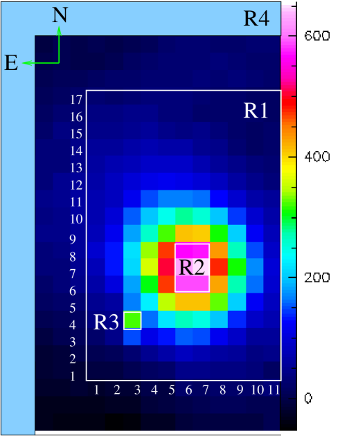
The subtraction of the background emission from the proplyd spectrum is a very challenging task (Henney & O’Dell, 1999). This problem arises since the background nebular emission is strongly inhomogeneous on an arc-second scale. In this work, we have used standard -method in order to fit an intensity versus position plane in a semi-rectangular field located away from the peak proplyd emission in each of the individual velocity channel maps. We assure that we only take samples of the background avoiding the region of the proplyd. These planar fits to the nebular emission are then subtracted from the corresponding velocity channel maps. In Figure 1, we show the observed field, the object orientation in the plane of the sky, and also the region that defines our background (region 4, labeled as R4 in Figure 1). Region 4 (see Figure 1) contains 76 spectra which are used to define the background. This Figure also shows an internal box (labeled as R1, or region 1), for which we have defined an arbitrary -coordinate system limited by (in the East direction) and (in the North direction; see Figure 1). In the following sections, we show maps of spatially distributed physical variables that will be constrained to the limits defined by this box. The spatial positions inside this domain will be defined using the -coordinate system described above. Regions 2 and 3 (labelled as R2 and R3 in Figure 1) define, respectively, a region near the center of the 167-317 proplyd and a region which has a high-velocity, redshifted feature (see below).
3 Observational results: spectral line identification and high velocity features
3.1 The emission lines intensities and ratios
The lines that we identify in the spectra have already been reported in previous papers of the Orion Nebula (e.g,. Baldwin et al., 2000). We select 4 different regions to measure the line intensities, namely, regions R1, R2, R3 and R4 (see Fig. 1 and §2 for the coordinate system definition).
Four spectra are then obtained by co-adding the spectra of the pixels included in each region. The spectrum of region 1 is the result of the sum of 187 pixels, for region 2 the sum of 6 pixels, region 3 represents the spectrum of a single pixel and region 4 the sum of 76 pixels. A set of 38 lines has been selected from a manual search for emission features in the spectrum integrated over the selected fields. The intensities of the emission lines are determined by fitting a flat continuum and integrating over the whole emission feature 444The radial velocity range that defines the integration limits in each intensity line determination varies from line to line, since the FWHM changes with the wavelength (see §2).. Then, a mean flux was obtained dividing the integrated flux by the total number of pixels of each region. Table 1 gives the list of the observed lines together with the mean flux of each region (after subtraction of the emission from the background, region R4) and the ratio to H (normalized to H). The fourth and eigth columns show the background emission and ratios to H, respectively, for each line. The mean fluxes are given in units of erg cm-2 s-1 px-1, and are not corrected for reddening. The absolute error of the mean flux is given in parentheses. This error was calculated taking into account the variations of the local continuum. The errors can be very large for the weaker lines. Also, the detection of spectral lines in region R3 is affected by the low signal to noise ratio. There are some lines which show stronger mean fluxes in the background, namely, the lines of Si III , Si II , [Ni II] and [Fe II] (see Table 1). These lines have low ionization potentials and are expected to appear mainly in regions of lower ionization degree. The lower line intensities within the proplyd indicate that these lines are mainly emitted by the background nebula, and that they are absorbed at least partially by the dust in the proplyd.
In Figure 2, we show the full extracted spectra from the data cube, for regions R1 to R4 as defined in Figure 1. In this figure, the spectra for regions R1, R2, R3 and R4 are depicted from bottom to top in each diagram. The data shown here are not background subtracted. Most of the detected 38 lines can be clearly seen in the spectra. It is also evident that the S/N is higher in regions R1 and R4 (which is due to the increase of the pixel number of these regions). Here, a third order cubic spline was fitted to the continuum and then subtracted from the data. Because of the high order spline polynome subtraction, some minor variations are still present near the H line.
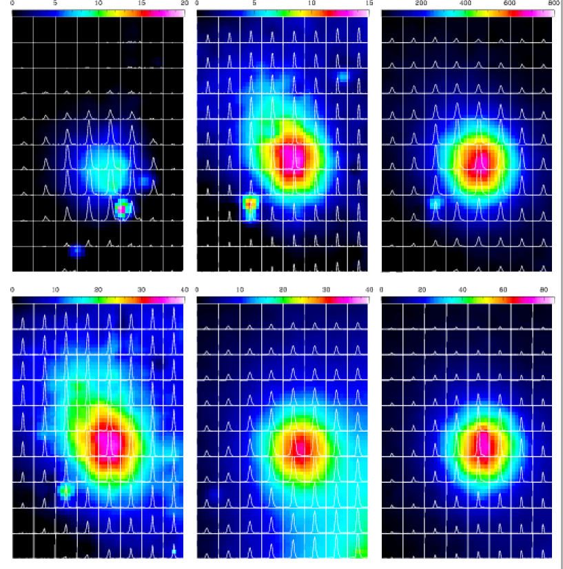
Figure 3 depicts (for region R1), 2D-intensity maps of the lines [N II]5755, [N II]6548, H, [N II]6583, [He I]7065 and [Ar III]7135, superimposed by line profiles. The data shown here are background subtracted, as described in §2. The line profiles can be better seen in Figure 4, in which we show the mean line profile for each line and for each of the regions R1, R2, R3 and R4, in the same diagram. As could be anticipated, the flux is more intense in region R2 (dotted line), where the proplyd is located, except for the [N II] line, which shows a stronger flux in region R3. For the H and [N II] lines the emission of region R3 is more intense than the emission of region R1. For lines with good S/N, the presence of a redshifted feature starts to become clear. An analisys of the profile components will be given in more detail below.
In order to see how the spectra of the different lines change spatially, in Figure 5 we present an intensity versus position plot for the same lines shown in Figures 3 and 4. We show how the intensity of these lines changes along a diagonal line, that crosses region R1 passing through the pixel (3,4) (region R3) and through the centre of region R2. We note that there are 2 intensity maxima for the H, [N II] and [N II] lines, clearly showing in which lines region R3 is clearly visible (also see Figure 3).
3.2 High velocity features
We associate region R3 with the redshifted jet of the proplyd, although in Figure 9 we will show that the emission of the jet is not restricted only to this pixel. A redshifted jet associated with the 167-317 proplyd was previously detected, with a propagation velocity of 100 km s-1 (e.g., Henney et al., 2002). We have also detected this high velocity feature in our data. In order to see this, we examine the behaviour of the moments of the radial velocity distribution. These are the flux-weighted mean radial velocity , the flux-weighted rms width of the line and the skewness , that are given, respectively, by:
| (1) |
| (2) |
| (3) |
where
| (4) |
The integrated intensity (see eq. 4 and Figure 3) shows that if we move away from the proplyd position (R2), the emission for several lines (for example, H and [Ar III]) rapidly drops to low values (close to the background value). We also note that the maps for the flux-weighted mean radial velocity 555Unless explicitly mentioned, the radial velocities presented here are not corrected for the systemic radial velocity, that is of the order of km s-1 (e.g., Meaburn et al., 1993). The error in the radial velocity measurements is of the order of 2.5 km s-1. (not shown here; see eq. 1) show that km s-1.
The flux-weighted rms width of the line and the skewness moment of the radial velocity distribution (see equations 2 and 3, respectively) are depicted in Figure 6, for the H (left) and [Ar III] (right) lines. Both of them were computed after carrying out both background and continuum subtractions. From Figure 6, we see that there is a clear enhancement of both of these moments from the proplyd position (R2 region) towards the R3 region (i.e., towards the SE direction, at a PA ). This behaviour of the moments leads us to infer that: 1) there is an increase in the line width as we go from the proplyd position to the SE direction; and 2) that there are redshifted wings in the line profiles. These results indicate the presence of a redshifted outflow in this region. We note that the same behaviour is seen in the He I 6678.15, [N II]6583.46 lines (not shown here).
In order to confirm the presence of high velocity components in the observed field, as well as to see the behaviour of the photoevaporated proplyd flow and the background emission, we have computed three-component Gaussian minimum fits for each position-dependent line profile. The profiles of all emission lines have a major peak at km s-1, the exact radial velocity of this peak changing with spatial position. In some spectral lines, there is an evident second peak at redshifted velocities ranging from 100 to 150 km s-1, corresponding to the jet associated with the proplyd. Finally, we have been able to detect a blueshifted component, which is fainter than the redshifted components. As an example of our three-component Gaussian fit, in Figure 7 we show the data (full line) and the fit (crosses), for the H and [Ar III]7135 lines in the (,)=(6,7) position. In this figure, for each emission line, the top-left panel represents the data and the three Gaussian fits, the top-right panel shows the main, low velocity component (and the Gaussian fit for this component), the bottom-left panel depicts the data minus the main component together with the fits for the blue- and red-shifted components and, finally, the bottom-right panel shows the residual, obtained by subtracting the three-component fit from the observed line profile. The fits depicted in this figure show the presence of redshifted and blueshifted components. The redshifted component is present in several lines in pixels around the SE direction, as already mentioned before. On the other hand, blueshifted emission can be found in several pixels to the NW of the proplyd peak emission as can be seen in the left bottom panel of Figure 7 and this could represent the first spectroscopic determination of the presence of a blueshifted counter-jet, with systemic velocities of -60 km s-1 km s-1. This blueshifted component is also suggested by the fitted profiles of HeI 7065 (not shown here).
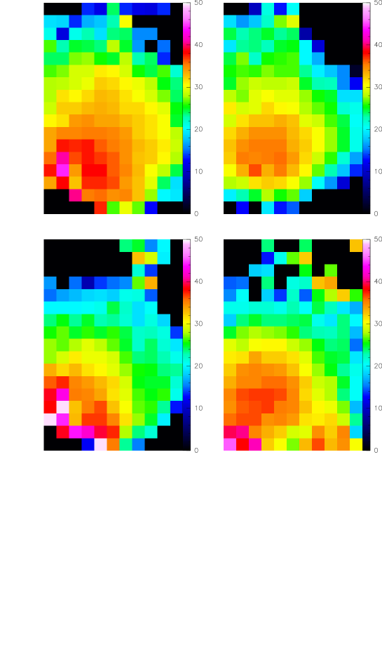
Figure 8 depicts the spatially distributed intensity over the R1 region (see Figure 1), of the main peak for the [N II]5754 (top-left), [N II]6548 (top-middle), H (top-right), [N II]6583 (bottom-left), HeI 7035 (bottom-middle) and [Ar III]7135 (bottom-right) lines. The values shown in this Figure were obtained from three-component Gaussian fits to the observed line profile. All of the lines peak at the proplyd position, at (,) = (6,7), inside the R2 region, and three of them (namely [N II]6548, top-middle; H, top-right; and [N II]6583, bottom-left), have a secondary, less intense peak at (,)=(3,4) (i.e., in the R3 region; see Figure 1 for the definition of the coordinate system). This secondary peak is probably related to the jet, since, as we have seen before, the jet propagates from the R2 region towards the SE direction. It is also interesting to note that there is a tail of faint emission (compared with the maximum in a given map) that extends in the NE direction, and that can be seen in both of the [N II] lines that bracket H (top-middle and bottom-left maps in Figure 8).
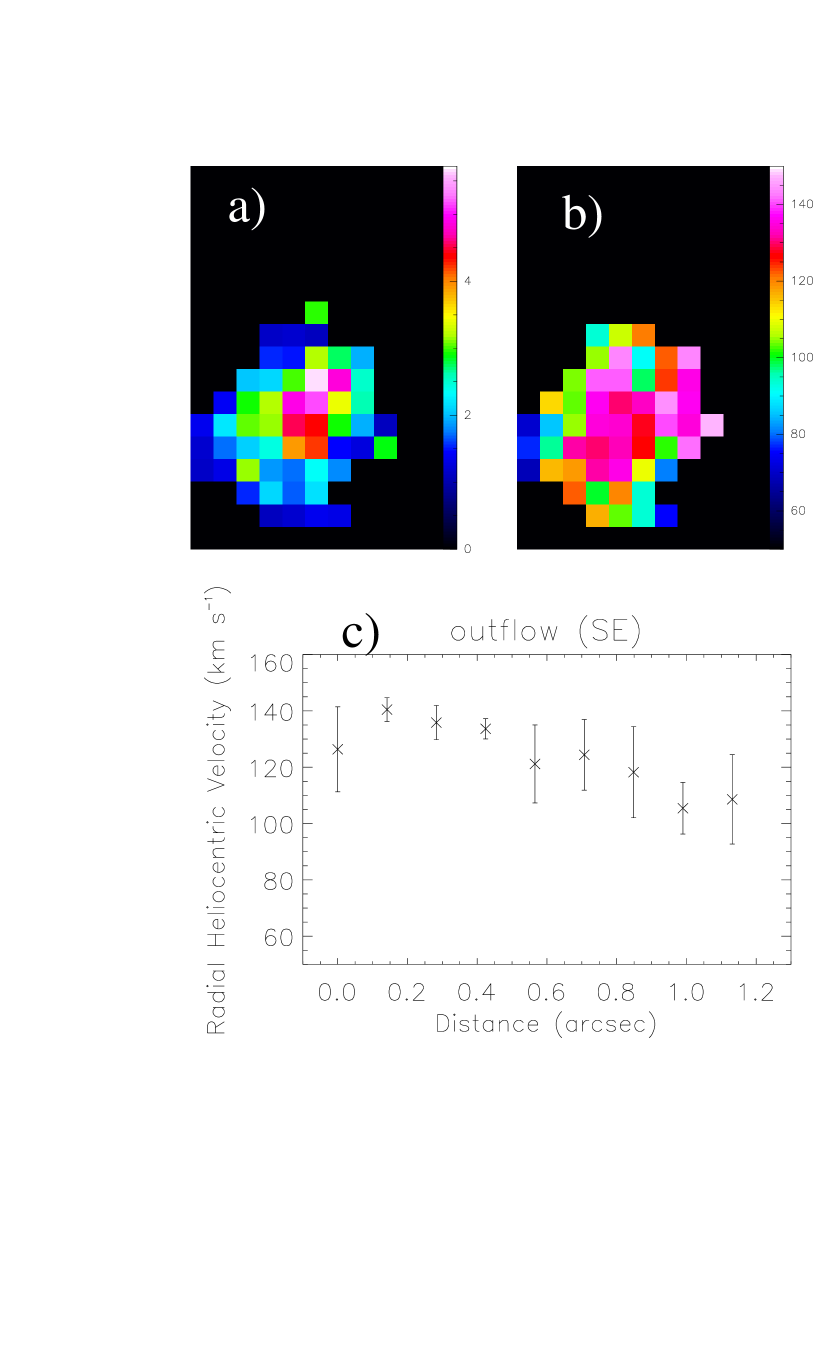
In Figure 9, we show the spatially dependent intensity (Fig. 9a) and the central velocity (Fig. 9b) of the redshifted component of the fitted H profile. We limit the maps to the spatial pixels which have a skewness km s-1. The pixels which satisfy this criterium have a well defined high velocity, redshifted component. These figures show that the high velocity component has an intensity maximum near the center of the proplyd, with an extension towards the SE direction (along the jet axis), surrounded by a region of decreasing fluxes. The high intensity spike seen in H, [N II] and [N II] lines (Figure 3) can be seen here. The jet shows a spread in velocity values, although most of the pixels present velocities around 120-140 km s-1. This figure also shows that the jet velocity decreases with increasing distance from the proplyd. This trend can be seen in the Figure 9c, where we show the radial velocity of the redshifted component as a function of distance from the proplyd position, (,) = (6,7) in region R1. To build this figure, we assume that the jet is propagating in a PA position angle. We define a box with one axis aligned with the jet axis, and the second, perpendicular dimension extending two pixels to each side of the jet axis. We then take averages (of the mean velocity of the redshifted component) perpendicular to the jet direction and plot the resulting velocity as a function of distance from the proplyd (see the bottom frame of Figure 8). There is an indication that the jet velocity is slowly diminishing as a function of distance from the source.
3.3 The spatial distribution of the nitrogen ratio
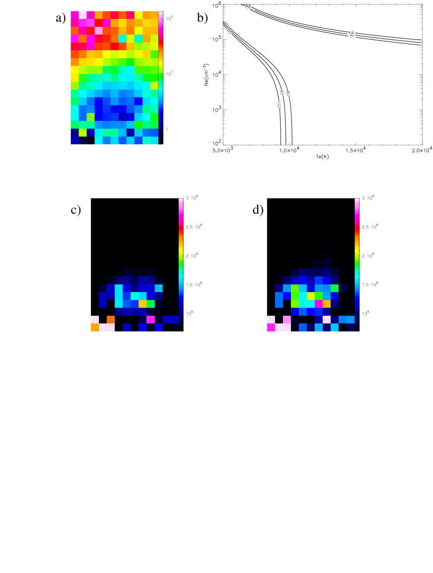
In Figure 10a, we show a map for the R1 region of the line ratio:
| (5) |
where and are the height and the dispersion of the fitted Gaussian profile (of the main, low velocity component). The [NII](6548+6583)/5754 ratio is a classical electron temperature diagnostic of low/medium density nebulae ( cm-3). At high densities, due to the collisional desexcitations, this ratio cannot be used for the determination of the electron temperature, but it turns out to be a quite good electron density diagnostic. This can be seen, for example, from the Osterbrock (1989) equation:
| (6) |
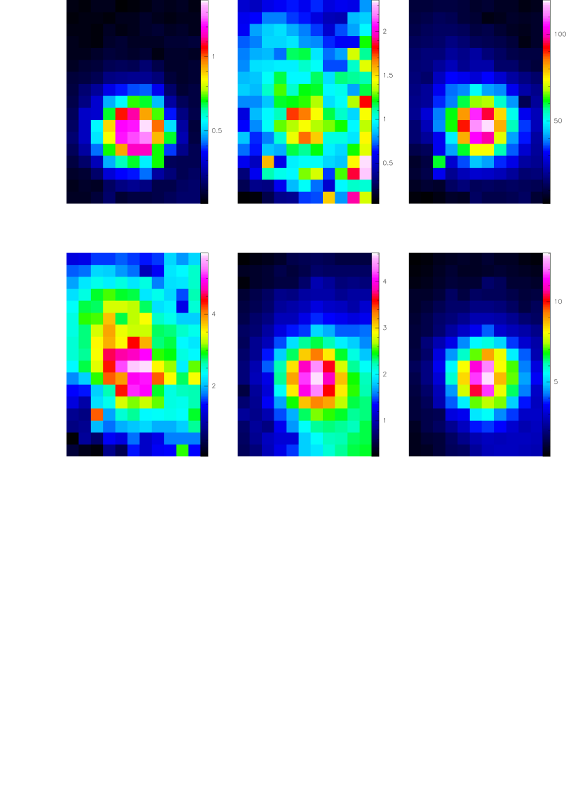
Figure 10b shows the lines corresponding to [NII](6548+6583)/5754 = 9, 10, 11, 80, 90, 100 in a plane. We can see that for the values obtained in our case (line ratios close to 10), the [NII](6548+6583)/5754 ratio is strongly dependent on the electron density, and that the dependence on the electron temperature is small.
In Figures 10c and 10d, we show the densities computed from the [NII](6548+6583)/5754 ratio for K and K, respectively. Although presenting a very complicated pattern, these figures show that the region coinciding with the proplyd center, and extending towards the SE direction (the jet propagation direction), shows the lowest line ratio, indicating electron densities () of the order of cm-3. This value is at least in qualitatively agreement with the cm-3 obtained by Henney et al. (2002) considering a K temperature for the ionization front (that is inside the R2 region). We can also note that both figures are similar, presenting few differences in the density values.
The extended structure from the R2 region towards the SE direction is surrounded by a region in which the nitrogen line ratio reaches values of up to . In this limit, cm-3. It is interesting to note that in the clump associated with the redshifted jet, the nitrogen line ratio increases substantially, indicating a decrease in the electron density when compared with the same values near the center of the proplyd. We have also obtained the [S II] emission maps. Unfortunately, we are not able to use these lines as a diagnostic because neither the ratio of this doublet is a good electron density indicator for this case (since it is constant for densities higher than 105 cm-3) nor do we have a good enough signal to noise ratio for these lines. Furthermore, the background subtracted spectra for these two lines give us negative fluxes in the proplyd region (see Table 1). The presence of these negative features in the line profiles is probably related with the presence of dust, as discussed by Henney & O’Dell (1999).
4 Discussion and conclusions
We have presented in this work the first Integral Field Unit (IFU) spectroscopic observations of a photoevaporating disk immersed in a HII region. In particular, we have taken advantage of the System Verification Run of the Gemini South Telescope Multi Object Spectrograph (GMOS) to obtain spectra of the 167-317 proplyd in the Orion nebula. The 167-317 proplyd, also known as LV2 (from the pioneering work from Laques & Vidal, 1979), is one of the brightest and best studied proplyds. In a single exposure, we took 400 spectra with a spatial resolution of . These spectra have been combined in order to optimize this instrumental feature, and, before discussing of our results, we want to make a few comments concerning the potential use of such IFU data-cubes for these objects. As previously discussed in the literature (Henney et al., 2002), the subtraction of the background emission is a very challenging task. This problem arises since the background near these proplyds (which are immersed in a highly non-homogeneous, photoionized ambient medium) is very complex and changes in an arc-second spatial scale. A careful computation of the background contribution to the spectra of these objects is one of the most important tasks in order to have reliable radial velocity measurements for both the proplyd photoevaporated flow and the high velocity features (jets) present in these systems. Here, we have used the 76 spectra, defined in Figure 1 as region R4, in order to obtain a planar fit for the background emission. We think that such a definition of the background emission is more precise, since we use several regions to calculate a better function to describe the background. One more thing to point out is that, with spatially distributed spectra, we are able to confidently separate the contribution of the background from the contribution of the object itself.
The data from the IFU observation of the 167-317 proplyd also allow us to investigate the spatially dependent properties of the outflows associated with this object. In particular, the 167-317 proplyd is known to have a redshifted, collimated jet that propagates with heliocentric velocities of km s-1 towards the SE direction, and with a spatial extension of (e.g, Meaburn, 1988; Meaburn et al., 1993; Massey & Meaburn, 1995; Henney, 2000; Henney et al., 2002). We find that a prominent, high velocity redshifted component can be detected in some emission lines, particularly in H, in this SE direction. The redshifted jet has a trend in its radial velocity (as a function of distance from the proplyd) with higher velocities close to the proplyd and lower velocities at increasing distances. We note that Henney et al. (2002) had previously suggested a variation in the jet velocity as a function of distance from the source.
There is a subtle peak (in several emission lines, particularly in [N II]5754 and H) that is associated with the SE jet emission, and located at SE of the center of the proplyd [at (x,y)=(3,4); the R3 region in Figure 1]. For this intensity peak, and also using the H profiles of the neighbouring pixels, we find a mean heliocentric velocity km s-1. It is interesting to note that previous HST images and spectroscopic analyses (Bally et al., 2000; Henney et al., 2002) also reveal a spike in the jet emission at from the proplyd cusp. If we associate these two emission regions as belonging to the same condensation, we can estimate a proper motion of km s-1, which combined with the km s-1 radial velocity give a full jet velocity of km s-1 (where the error was inferred from the spatial resolution of our data). This velocity is of the same order as the values inferred for Herbig-Haro jets associated with T Tauri stars. However, the exact nature of this spike is unknown. We could relate this spike with a bow shock of the jet, since the line profiles for both are similar (Hartigan et al., 1987; Beck et al., 2004), showing a low velocity, more intense peak together with a high velocity, less intense peak (similar to the line profiles seen in Figures 3, 4 and 7).
We have found evidence for a blueshifted component in several emission lines around the northwest tip of the proplyd position. In particular, the H profiles reveal the presence of a blue-shifted component with systemic velocity km s-1, which indicates that its velocity is similar though smaller than the one of the redshifted jet. However, the intensities of the blue-shifted features are much lower than the intensity of the redshifted components associated with the SE jet: the counter-jet is at least four times less intense than the redshifted jet (in H). The presence of such a blue-shifted component very close to the LV2 proplyd, together with previously reported evidence that (at several arcseconds to the NW of this proplyd; see Massey & Meaburn 1995) there is a blueshifted component (in the [O III]5007 line) strongly suggests the existence of a faint counterjet.
It is interesting to estimate the mass loss rate for the proplyd and the associated redshifted jet. In order to do this, we consider a simple model that assumes that the proplyd flow arises from a hemispherical, constant velocity wind that originates at the proplyd ionization front, at a radius . Using the H luminosity , we can then obtain the particle density at this point and the mass loss rate, from:
| (7) |
where accounts for the extintion correction, cm3 is the effective recombination coefficient for H, is the energy of the H transition, is the mean molecular weight and km s-1 is a typical value for the sound velocity in an HII region. The extintion correction is obtained from the base 10 logarithm of the extintion at () which for the proplyd 167-317 is equal to 0.83 (O’Dell, 1998) through the relation, (O’Dell et al., 1992), where here we take = 0.56. Assuming for the ionization front radius a value cm (Henney et al., 2002) we obtain cm-3 and M☉ year-1. Henney et al. (2002) have obtained a M☉ year-1 , and the small differences between both results may arise from the different observational techniques employed in both cases.
For the redshifted jet, we assume that the outflow arises from the blob located in region R3 (or pixel 3,4). In this case, the particle density, mass and mass loss rate of the jet are given by,
| (8) |
| (9) |
| (10) |
where cm is the radius of the blob, km s-1 and cm are the propagation velocity and length of the jet, respectively, derived above. With these values, we obtain for the jet a mass loss rate equal to M☉ year-1, which is similar to the mass loss rate of typical HH jets from T Tauri stars.
We have been able to construct a ([NII] + [NII])/[NII] line ratio map. This ratio indicates densities higher than cm-3 for the proplyd emission region, consistent with values previously reported in the literature. We find a subtle enhancement of this ratio in the region of the redshifted jet. Further observations of electron temperature and density diagnostic lines would allow a more accurate determination of the spatial dependence of these important parameters.
References
- Baldwin et al. (2000) Baldwin, J. A., Verner, E. M., Verner, D. A., Ferland, G. J., Martin, P. G., Korista, K. T., & Rubin, R. H. 2000, ApJS, 129, 229
- Bally et al. (1998) Bally, J., Sutherland, R.S., Devine, D., & Johnstone, D. 1998, AJ, 116, 293
- Bally et al. (2000) Bally, J., O’Dell, C.R., & McCaughrean, M.J., 2000, AJ, 119, 2919
- Bally et al. (2005) Bally, J., Licht, D., Smith, N., & Walawender, J. 2005, AJ, 129, 355
- Beck et al. (2004) Beck, T. L., Riera, A., Raga, A. C., & Aspin, C. 2004, AJ, 127, 408
- Churchwell et al. (1987) Churchwell, E., Felli, M., Wood, D.O.S., & Massi, M. 1987, ApJ, 321, 516
- Hartigan et al. (1987) Hartigan, P, Raymond, J., & Hartmann, L. 1987, ApJ, 316, 323
- Henney (2000) Henney, W. J. 2000, Rev. Mex. Astron. Astrof. (Serie de Conferencias), 9, 198
- Henney & Arthur (1998) Henney, W.J., & Arthur, S.J., 1998, AJ, 116, 322
- Henney & O’Dell (1999) Henney, W.J., & O’Dell, C.R., 1999, AJ, 118, 2350
- Henney et al. (2002) Henney, W.J., O’Dell, C.R., Meaburn, J., Garrington, S.T., & Lopez, J.A. 2002, ApJ, 566, 315
- Johnstone et al. (1998) Johnstone, D., Hollenbach, D., & Bally, J., 1998, ApJ, 499, 758
- Laques & Vidal (1979) Laques, P., & Vidal, J.L. 1979, A&A, 73, 97
- Massey & Meaburn (1995) Massey, R.M., & Meaburn, J. 1995, MNRAS, 273, 615
- Meaburn (1988) Meaburn, J. 1988, MNRAS, 233, 791
- Meaburn et al. (1993) Meaburn, J., Massey, R.M., Raga, A.C., & Clayton, C.A. 1993, MNRAS, 260, 625
- Meaburn et al. (2002) Meaburn, J., Graham, M. F., & Redman, M. P. 2002, MNRAS, 337, 327
- O’Dell (1998) O’Dell, C.R. 1998, AJ, 115, 263
- O’Dell et al. (1993) O’Dell, C. R., Wen, Z., & Hu, X. 1993, ApJ, 410, 696
- O’Dell & Wen (1994) O’Dell, C. R., & Wen, Z. 1994, ApJ, 436, 194
- O’Dell et al. (1992) O’Dell, C. R., Walter, D. K., & Dufour, R. J. 1992, ApJ, 399, L67
- Osterbrock (1989) Osterbrock, D.E. 1989, in Astrophysics of Gaseous Nebulae and Active Galactic Nuclei (Univ. Science Books: Mill Valley, California)
- Richling & Yorke (2000) Richling, S., & Yorke, H. W. 2000, ApJ, 539, 258
- Smith et al. (2003) Smith, N., Bally, J., & Morse, J.A. 2000, ApJ, 587, L105
- Smith et al. (2005) Smith, N., Bally, J., Licht, D., & Walawender, J. 2005, AJ, 129, 382.
- Störzer & Hollenbach (1998) Störzer, H., & Hollenbach, D. 1998, ApJ, 502, L71
| Line | Mean Flux ( erg cm-2 s-1 px-1) | Line ratio (H) | |||||||
|---|---|---|---|---|---|---|---|---|---|
| Ion | (Å) | R1aa The regions R1, R2, R3 and R4 are defined in Figure 1. | R2 | R3 | R4 | R1 | R2 | R3 | R4 |
| [Cl III] | 5537.70 | -bb The symbol - implies that . | 0.024 (0.007)cc The terms inside the parentheses are the absolute errors of the intensity of each line, for each one of the regions. | - | 0.155 (0.007) | - | 0.012 (0.003) | - | 0.164 (0.007) |
| N II | 5666.63 | 0.024 (0.004) | 0.033 (0.003) | NDdd The symbol ND implies that the line were not detected in that region. | 0.007 (0.003) | 0.058 (0.009) | 0.016 (0.002) | ND | 0.007 (0.003) |
| N II | 5679.56 | - | 0.002 (0.004) | ND | 0.012 (0.004) | - | 0.001 (0.002) | ND | 0.012 (0.004) |
| Si III | 5739.73 | - | - | ND | 0.038 (0.002) | - | - | ND | 0.040 (0.002) |
| [N II] | 5754.59 | 0.535 (0.003) | 2.50 (0.01) | 0.638 (0.004) | 0.186 (0.003) | 1.283 (0.008) | 1.245 (0.005) | 0.598 (0.004) | 0.196 (0.003) |
| He I | 5875.64 | 1.451 (0.003) | 7.80 (0.01) | 1.39 (0.03) | 4.327 (0.001) | 3.48 (0.01) | 3.879 (0.008) | 1.30 (0.03) | 4.568 (0.005) |
| O I | 5958.60 | 0.007 (0.003) | 0.033 (0.007) | ND | 0.013 (0.003) | 0.016 (0.008) | 0.016 (0.004) | ND | 0.013 (0.003) |
| Si II | 5978.93 | - | - | ND | 0.028 (0.002) | - | - | ND | 0.030 (0.002) |
| O I | 6046.44 | 0.014 (0.002) | 0.09 (0.01) | ND | 0.020 (0.001) | 0.034 (0.004) | 0.045 (0.005) | ND | 0.021 (0.001) |
| [O I] | 6300.30 | 0.306 (0.004) | 1.58 (0.02) | 0.38 (0.02) | 0.086 (0.001) | 0.73 (0.01) | 0.78 (0.01) | 0.35 (0.02) | 0.091 (0.002) |
| [S III] | 6312.06 | 0.44 (0.02) | 2.11 (0.08) | 0.29 (0.04) | 0.516 (0.006) | 1.05 (0.04) | 1.05 (0.04) | 0.28 (0.04) | 0.545 (0.006) |
| Si II | 6347.11 | - | 0.03 (0.01) | ND | 0.063 (0.004) | - | 0.015 (0.005) | ND | 0.066 (0.004) |
| [O I] | 6363.78 | 0.09 (0.01) | 0.51 (0.02) | 0.03 (0.03) | 0.03 (0.01) | 0.21 (0.03) | 0.25 (0.01) | 0.03 (0.02) | 0.03 (0.01) |
| Si II | 6371.37 | - | 0.03 (0.01) | ND | 0.026 (0.003) | - | 0.018 (0.007) | ND | 0.027 (0.003) |
| [N II] | 6548.05 | 1.00 (0.01) | 2.55 (0.02) | 2.53 (0.04) | 3.475 (0.009) | 2.39 (0.03) | 1.27 (0.01) | 2.34 (0.04) | 3.67 (0.01) |
| H I | 6562.82 | 41.73 (0.02) | 201.20 (0.05) | 106.66 (0.02) | 94.73 (0.01) | 100.0 (0.4) | 100.0 (0.1) | 100.0 (0.1) | 100.0 (0.1) |
| C II | 6578.05 | 0.02 (0.01) | 0.10 (0.02) | 0.05 (0.01) | 0.09 (0.01) | 0.04 (0.03) | 0.05 (0.01) | 0.05 (0.01) | 0.09 (0.01) |
| [N II] | 6583.45 | 3.134 (0.005) | 8.48 (0.02) | 5.304 (0.007) | 10.710 (0.001) | 7.51 (0.03) | 4.21 (0.01) | 4.972 (0.009) | 11.30 (0.01) |
| He I | 6678.15 | 0.530 (0.007) | 2.621 (0.009) | 0.42 (0.02) | 1.241 (0.007) | 1.27 (0.02) | 1.303 (0.005) | 0.40 (0.02) | 1.310 (0.008) |
| [S II] | 6716.44 | 0.016 (0.005) | 0.029 (0.006) | - | 0.425 (0.003) | 0.04 (0.01) | 0.015 (0.003) | - | 0.448 (0.004) |
| [S II] | 6730.82 | 0.044 (0.002) | 0.06 (0.02) | - | 0.945 (0.002) | 0.107 (0.006) | 0.032 (0.008) | - | 0.998 (0.002) |
| He I | 6989.48 | - | 0.016 (0.002) | ND | 0.005 (0.000)ee Absolute error smaller than . | - | 0.008 (0.001) | ND | 0.005 (0.000)ee Absolute error smaller than . |
| O I | 7002.12 | 0.014 (0.004) | 0.088 (0.005) | 0.01 (0.01) | 0.022 (0.001) | 0.03 (0.01) | 0.044 (0.003) | 0.01 (0.01) | 0.023 (0.001) |
| He I | 7065.18 | 0.995 (0.004) | 5.393 (0.009) | 0.39 (0.03) | 2.439 (0.001) | 2.38 (0.01) | 2.680 (0.005) | 0.37 (0.03) | 2.574 (0.003) |
| [Ar III] | 7135.79 | 3.713 (0.004) | 19.39 (0.02) | 1.88 (0.01) | 5.277 (0.003) | 8.90 (0.04) | 9.64 (0.01) | 1.76 (0.01) | 5.570 (0.007) |
| [Fe II] | 7155.16 | - | 0.06 (0.03) | ND | 0.005 (0.005) | - | 0.03 (0.01) | ND | 0.005 (0.006) |
| He I | 7160.60 | 0.003 (0.004) | 0.007 (0.008) | ND | 0.017 (0.004) | 0.006 (0.009) | 0.004 (0.004) | ND | 0.018 (0.004) |
| C II | 7231.33 | 0.004 (0.005) | 0.04 (0.01) | ND | 0.046 (0.004) | 0.01 (0.01) | 0.019 (0.005) | ND | 0.049 (0.004) |
| [C II] | 7236.42 | 0.024 (0.004) | 0.140 (0.005) | - | 0.108 (0.004) | 0.06 (0.01) | 0.070 (0.002) | - | 0.115 (0.004) |
| O I | 7254.45 | 0.028 (0.001) | 0.17 (0.01) | ND | 0.027 (0.001) | 0.066 (0.003) | 0.086 (0.007) | ND | 0.028 (0.001) |
| He I | 7281.35 | 0.13 (0.01) | 0.73 (0.02) | 0.04 (0.04) | 0.235 (0.007) | 0.32 (0.02) | 0.365 (0.008) | 0.03 (0.03) | 0.248 (0.008) |
| He I | 7298.05 | 0.006 (0.004) | 0.040 (0.007) | ND | 0.020 (0.001) | 0.01 (0.01) | 0.020 (0.003) | ND | 0.021 (0.001) |
| [O II] | 7319.99 | 3.94 (0.04) | 21.9 (0.2) | 2.032 (0.008) | 1.488 (0.004) | 9.4 (0.1) | 10.89 (0.09) | 1.905 (0.008) | 1.571 (0.005) |
| [O II] | 7330.30 | 2.99 (0.08) | 16.38 (0.08) | 1.45 (0.08) | 1.12 (0.08) | 7.2 (0.2) | 8.14 (0.04) | 1.36 (0.07) | 1.18 (0.08) |
| [Ni II] | 7377.83 | 0.003 (0.001) | ND | ND | 0.013 (0.000)ee Absolute error smaller than . | 0.007 (0.002) | ND | ND | 0.014 (0.000)ee Absolute error smaller than . |
| [N I] | 7442.00 | 0.005 (0.003) | 0.024 (0.009) | ND | 0.008 (0.003) | 0.012 (0.008) | 0.012 (0.004) | ND | 0.008 (0.004) |
| [N I] | 7468.31 | 0.009 (0.002) | 0.049 (0.007) | ND | 0.011 (0.001) | 0.022 (0.004) | 0.024 (0.003) | ND | 0.012 (0.001) |
| [C II] | 7530.00 | 0.012 (0.000)ee Absolute error smaller than . | 0.014 (0.001) | ND | 0.010 (0.000)ee Absolute error smaller than . | 0.030 (0.001) | 0.007 (0.000)ee Absolute error smaller than . | ND | 0.011 (0.000)ee Absolute error smaller than . |