Fast directional continuous spherical wavelet transform algorithms

Abstract

We describe the construction of a spherical wavelet analysis through the inverse stereographic projection of the Euclidean planar wavelet framework, introduced originally by Antoine and Vandergheynst and developed further by Wiaux et al.. Fast algorithms for performing the directional continuous wavelet analysis on the unit sphere are presented. The fast directional algorithm, based on the fast spherical convolution algorithm developed by Wandelt and Górski, provides a saving of $\mathcal{O}(\sqrt{{N_{\rm{pix}}}})$ over a direct quadrature implementation for ${N_{\rm{pix}}}$ pixels on the sphere, and allows one to perform a directional spherical wavelet analysis of a $10^{6}$ pixel map on a personal computer.

I Introduction

Wavelet analysis has proven useful in many applications due to the ability of wavelets to resolve localised signal content in both scale and space. Many of these applications, however, are restricted to data defined in Euclidean space: the 1-dimensional line, the 2-dimensional plane and, occasionally, higher dimensions. Nevertheless, data are often measured or defined on other manifolds, such as the 2-sphere. Examples where data are measured on the sphere are found in astrophysics (e.g. [1, 2]), planetary science (e.g. [3, 4, 5]), geophysics (e.g. [6, 7, 8]), computer vision (e.g. [9]) and quantum chemistry (e.g. [10, 11]). To realise the potential benefits that may be provided by wavelets in such settings, ordinary Euclidean wavelet analysis must be extended to spherical geometry.

A number of attempts have been made to extend wavelets to the unit sphere. Discrete second generation wavelets on the sphere that are based on a multiresolution analysis have been developed [12, 13]. Other authors have focused on the continuous wavelet transform on the sphere. A number of works construct a solution using a harmonic approach [14, 15, 16, 17], however these solutions suffer from the poor localisation of the spherical harmonic functions. Others adopt a tangent bundle viewpoint [18, 19], thereby avoiding the necessity to define a dilation operator on the sphere. A satisfactory extension of the continuous wavelet transform to the sphere is defined by [20], however this construction requires an abstract dilation parameter that must satisfy a number of ad hoc assumptions. More recently, a consistent and satisfactory framework for wavelets defined on the unit sphere has been constructed and developed by [21, 22, 23, 24, 25, 26, 27]. Moreover, this construction is derived entirely from group theoretic principles and inherently satisfies a number of natural requirements. We consider the continuous spherical wavelet transform (CSWT) developed in these last works. For a more detailed review of the attempts made at constructing a wavelet transform on the unit sphere see [21, 22, 28].

Current and future data-sets defined on the sphere are of considerable size. The current Wilkinson Microwave Anisotropy Probe (WMAP) data of the cosmic microwave background (CMB) contain approximately $3\times 10^{6}$ pixels on the sphere, whereas the forthcoming Planck CMB mission will generate maps with approximately $50\times 10^{6}$ pixels. Fast algorithms are therefore required to perform the CSWT on practical data-sets. A semi-fast algorithm to implement the CSWT is presented in [23] and implemented in the YAWTb (Yet-Another-Wavelet-Toolbox) Matlab wavelet toolbox (which also makes use of the SpharmonicKit). However, this implementation is restricted to an equi-angular tessellation of the sphere. The beauty of this tessellation is its simplicity and ability to be easily represented in matrix form. However, the pixels of an equi-angular tessellation are densely spaced about the poles and do not have equal areas. Other tessellations of the sphere also exist, such as those constructed to minimise some energy measure [29, 30, 31] or those constructed for more practical or numerical purposes (for example the IGLOO [32], HEALPix [33] and GLESP [34] schemes). There is thus a need for a fast implementation of the CSWT that is not tied to any particular tessellation of the sphere.

We fill this void by presenting a fast algorithm for performing the directional CSWT. The CSWT at a particular scale is essentially a spherical convolution, hence we may apply the fast spherical convolution algorithm developed by [35] to evaluate the wavelet transform. The algorithm is posed in harmonic space and thus is independent of the underlying tessellation of the sphere, (although an iso-latitude tessellation does enable faster spherical harmonic transforms, thereby increasing the speed of the algorithm). The framework supports both non-azimuthally symmetric spherical wavelets and a decomposition that employs anisotropic dilations, however no synthesis is possible when anisotropic dilations are incorporated. For an illustration of a spherical wavelet analysis on a practical problem of considerable size we refer the reader to our recent works to test the CMB for deviations from Gaussianity [36, 37] and to detect the integrated Sachs-Wolfe (ISW) effect [38]. Both of these works involve performing 1000 Monte Carlo simulations and would not have been feasible without a fast directional CSWT algorithm.

The remainder of this paper is structured as follows. In section II we describe the CSWT in the framework presented by [27]. For a more complete treatment of the spherical wavelet transform in this framework and the correspondence between spherical and Euclidean wavelets we recommend that the reader refer to [27]. We also present an extension to anisotropic dilations, however in this case the basis functions are not strictly wavelets hence perfect reconstruction is not possible. Various algorithms to perform the CSWT are described and then compared in section III. An application of our implementation is demonstrated in section IV. Concluding remarks are made in section V.

II The continuous spherical wavelet transform

To extend Euclidean wavelet analysis to spherical geometry a number of requirements must be satisfied: (i) the signals and wavelets must live fully on the unit sphere; (ii) the transform must involve local dilations of some kind on the unit sphere; and (iii) the spherical wavelet transform should reduce locally to the Euclidean transform on the tangent plane (i.e. the Euclidean limit must be satisfied) [20]. The final requirement is intuitively obvious; the sphere is asymptotically flat, hence any spherical wavelet transform should match the planar Euclidean transform on small scales, or equivalently, for a large radius of curvature.

The spherical wavelet transform developed in [21, 22, 23, 24, 25, 26] satisfies all of these requirements, moreover each requirement naturally follows from the construction. The construction of this transform is derived entirely from group theoretical principles. However, in a recent work by [27] this formalism is reintroduced independently of the original group theoretic formalism, in an equivalent, practical and self-consistent approach. We adopt this approach herein.

The correspondence principle between spherical and Euclidean wavelets is developed by [27], relating the concepts of planar Euclidean wavelets to spherical wavelets through a stereographic projection. We use the stereographic projection to define affine transformations on the unit sphere that facilitate the construction of a wavelet basis on the unit sphere. The spherical wavelet transform may then be defined as the projection on to this basis, where the spherical wavelets must satisfy the appropriate admissibility criterion to ensure perfect reconstruction.

II-A Stereographic projection

In order to construct a correspondence between wavelets on the plane ($\mathbb{R}^{2}$) and sphere (${S^{2}}$) a projection operator between the two spaces must be chosen. It is shown in [27] that the stereographic projection is the unique unitary, radial and conformal diffeomorphism between the sphere and the plane.

The stereographic projection is defined by projecting a point on the unit sphere to a point on the tangent plane at the north pole, by casting a ray though the point and the south pole. The point on the unit sphere is mapped on to the intersection of this ray and the tangent plane (see Fig. 1). Formally, we may define the stereographic projection operator as $\Pi:\omega\rightarrow\mathbf{x}=\Pi\omega=(r(\theta),\phi)$ where $r=2\tan(\theta/2)$, $\omega\equiv(\theta,\phi)\in{S^{2}}$ denotes spherical coordinates with colatitude $\theta$ and longitude $\phi$ and $\mathbf{x}\in\mathbb{R}^{2}$ is a point in the plane, denoted here by the polar coordinates $(r,\phi)$. The inverse operator is $\Pi^{-1}:\mathbf{x}\rightarrow\omega=\Pi^{-1}\mathbf{x}=(\theta(r),\phi)$, where $\theta(r)=2\tan^{-1}(r/2)$.

Following the formulation of [27] again, we define the action of the stereographic projection operator on functions on the plane and sphere. We consider the space of square integrable functions in $L^{2}(\mathbb{R}^{2},\mathrm{\,d}^{2}\mathbf{x})$ on the plane and $L^{2}({S^{2}},\mathrm{\,d}\Omega)$ on the unit sphere, where $\mathrm{\,d}\Omega=\sin\theta\mathrm{\,d}\theta\mathrm{\,d}\phi$ is the usual rotation invariant measure on the sphere. The action of the stereographic projection operator $\Pi:s\in L^{2}({S^{2}},\mathrm{\,d}\Omega)\rightarrow p=\Pi s\in L^{2}(\mathbb{R}^{2},\mathrm{\,d}^{2}\mathbf{x})$ on functions is defined as

$$p(r,\phi)=(\Pi s)(r,\phi)=(1+r^{2}/4)^{-1}s(\theta(r),\phi)\>.$$ (1)

The inverse stereographic projection operator $\Pi^{-1}:p\in L^{2}(\mathbb{R}^{2},\mathrm{\,d}^{2}\mathbf{x})\rightarrow s=\Pi^{-1}p\in L^{2}({S^{2}},\mathrm{\,d}\Omega)$ on functions is then

$$s(\theta,\phi)=(\Pi^{-1}p)(\theta,\phi)=[1+\tan^{2}(\theta/2)]p(r(\theta),\phi)\>.$$ (2)

The pre-factors introduced ensure that the $L^{2}$-norm of functions through the forward and inverse projections are conserved. In the Euclidean limit, the stereographic projection and inverse naturally reduce to the identity operator [21].

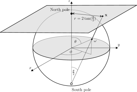
Figure 1: Stereographic projection of the sphere onto the plane.

II-B Affine transformations on the sphere

A wavelet basis is constructed on the unit sphere in section II-C by applying the spherical extension of Euclidean translations and dilations to mother wavelets defined on the unit sphere. The extension of these affine transformations to the sphere, facilitated by the stereographic projection operator, are defined here.

The natural extension of Euclidean translations on the unit sphere are rotations. These are characterised by the elements of the rotation group $\mathrm{SO}(3)$, which we parameterise in terms of the three Euler angles $\rho=(\alpha,\beta,\gamma)$. The rotation of a square-integrable function $s\in L^{2}({S^{2}},\mathrm{\,d}\Omega)$ is defined by

$$[R(\rho)s](\omega)=s(\rho^{-1}\omega),\;\;\rho\in\mathrm{SO}(3)\>.$$ (3)

Dilations on the unit sphere are constructed by first lifting the sphere to the plane by the stereographic projection, followed by the usual Euclidean dilation in the plane, before re-projecting back onto the sphere. We generalise to anisotropic dilations on the sphere (a similar anisotropic dilation operator on the sphere has been independently proposed by [39]), however in this setting we do not achieve a wavelet basis and hence cannot synthesise our original signal. We define the anisotropic Euclidean dilation operator in $L^{2}(\mathbb{R}^{2},\mathrm{\,d}^{2}\mathbf{x})$ as

$$[d(a,b)p](x,y)=a^{-1/2}b^{-1/2}\>p(a^{-1}x,b^{-1}y)\>,$$ (4)

for the non-zero positive scales $a,b\in\mathbb{R}^{+}_{\ast}$. The $a^{-1/2}b^{-1/2}$ normalisation factor ensures the $L^{2}$-norm is preserved. The spherical dilation operator $\mathcal{D}({a,b}):s(\theta,\phi)\rightarrow[\mathcal{D}({a,b})s](\theta,\phi)$ in $L^{2}({S^{2}},\mathrm{\,d}\Omega)$ is defined as the conjugation by $\Pi$ of the Euclidean dilation $d({a,b})$ in $L^{2}(\mathbb{R}^{2},\mathrm{\,d}^{2}\mathbf{x})$ on the tangent plane at the north pole:

$$\mathcal{D}({a,b})=\Pi^{-1}\,d({a,b})\,\Pi\>.$$ (5)

The norm of functions in $L^{2}({S^{2}},\mathrm{\,d}\Omega)$ is preserved by the spherical dilation as both the stereographic projection operator and Euclidean dilations preserve the norm of functions. Extending the isotropic spherical dilation operator defined by [27] to anisotropic dilations, we obtain

$$[\mathcal{D}({a,b})s](\omega)=[\lambda({a,b},\theta,\phi)]^{1/2}\>s(\omega_{1/a,1/b})\>,$$ (6)

where $\omega_{a,b}=(\theta_{a,b},\phi_{a,b})$,

$$\tan(\theta_{a,b}/2)=\tan(\theta/2)\sqrt{a^{2}\cos^{2}{\phi}+b^{2}\sin^{2}{\phi}}$$

and

$$\tan(\phi_{a,b})=\frac{b}{a}\tan(\phi)\>.$$

For the case where $a=b$ the anisotropic dilation reduces to the usual isotropic case defined by $\tan(\theta_{a}/2)=a\tan(\theta/2)$ and $\phi_{a}=\phi$. The $\lambda({a,b},\theta,\phi)$ cocycle term follows from the factors introduced in the stereographic projection of functions to preserve the $L^{2}$-norm. Alternatively, the cocycle may be derived explicitly to preserve the $L^{2}$-norm when the stereographic projection of functions do not have these pre-factor terms. The cocycle of an anisotropic spherical dilation is defined by

$$\lambda({a,b},\theta,\phi)=\frac{4a^{3}b^{3}}{\left(A_{-}\cos\theta+A_{+}\right)^{2}}\>,$$ (7)

where

$$A_{\pm}=a^{2}b^{2}\pm a^{2}\sin^{2}\phi\pm b^{2}\cos^{2}\phi\>.$$

For the case where $a=b$ the anisotropic cocycle reduces to the usual isotropic cocycle

$$\lambda(a,a,\theta,\phi)=\frac{4a^{2}}{[(a^{2}-1)\cos{\theta}+a^{2}+1]^{2}}\>.$$

Although the ability to perform anisotropic dilations is of practical use, we do not achieve a wavelet basis in this setting. In the anisotropic setting a bounded admissibility integral cannot be determined (even in the plane), thus the synthesis of a signal from its coefficients cannot be performed. This results from there being no direct means of evaluating the proper measure in the absence of a group structure. The projection of a signal onto basis functions undergoing anisotropic dilations may be performed in an analogous manner to the following discussion of the wavelet transform. However, since these basis functions are not wavelets we restrict the following discussion to isotropic dilations.

II-C Wavelet transform

A wavelet basis on the unit sphere may now be constructed from rotations and isotropic dilations (where $a=b$) of a mother spherical wavelet $\psi\in L^{2}({S^{2}},\mathrm{\,d}\Omega)$. The corresponding wavelet family $\{\psi_{a,\rho}\equiv R(\mathbf{\rho})\mathcal{D}(a,a)\psi,\;{\rho\in\mathrm{SO}(3),}\;{a\in\mathbb{R}_{\ast}^{+}}\}$ provides an over-complete set of functions in $L^{2}({S^{2}},\mathrm{\,d}\Omega)$. The CSWT of $s\in L^{2}({S^{2}},\mathrm{\,d}\Omega)$ is given by the projection onto each wavelet basis function in the usual manner,

$${W_{\psi}^{s}}(a,\mathbf{\rho})\equiv\int_{{S^{2}}}\mathrm{\,d}\Omega\>\psi_{a,\mathbf{\rho}}^{\ast}(\omega)\>s(\omega)=\left<\psi_{a,\mathbf{\rho}}\mid s\right>\>,$$ (8)

where the $\ast$ denotes complex conjugation.

The transform is general in the sense that all orientations in the rotation group $\mathrm{SO}(3)$ are considered, thus directional structure is naturally incorporated. It is important to note, however, that only local directions make any sense on ${S^{2}}$. There is no global way of defining directions on the sphere – there will always be some singular point where the definition fails.

The synthesis of a signal on the unit sphere from its wavelet coefficients is given by

$$s(\omega)=\int_{\mathrm{SO}(3)}\mathrm{\,d}\mathbf{\rho}\int_{0}^{\infty}\frac{\mathrm{\,d}a}{a^{3}}\>\>{W_{\psi}^{s}}(a,\mathbf{\rho})\>[R(\mathbf{\rho})L_{\psi}\psi_{a}](\omega)\>,$$ (9)

where $\mathrm{\,d}\mathbf{\rho}=\sin\beta\mathrm{\,d}\alpha\mathrm{\,d}\beta\mathrm{\,d}\gamma$. The $L_{\psi}$ operator in $L^{2}({S^{2}},\mathrm{\,d}\Omega)$ is defined by the action

$$(\widehat{L_{\psi}f})_{\ell m}=\widehat{f}_{\ell m}/C_{\psi}^{\ell}$$ (10)

on the spherical harmonic coefficients of functions $f\in L^{2}({S^{2}},\mathrm{\,d}\Omega)$, where $C_{\psi}^{\ell}$ is defined below. The hat denotes the spherical harmonic coefficients

$$\widehat{f}_{\ell m}=\int_{{S^{2}}}\mathrm{\,d}\Omega\>Y_{\ell m}^{\ast}(\omega)\>f(\omega)=\left<Y_{\ell m}\mid f\right>$$

of the decomposition

$$f(\omega)=\sum_{\ell=0}^{\infty}\sum_{m=-\ell}^{\ell}\widehat{f}_{\ell m}Y_{\ell m}(\omega)\>.$$

We adopt the Condon-Shortley phase convention where the normalised spherical harmonics are defined by

$$Y_{{\ell m}}(\omega)=(-1)^{m}\sqrt{\frac{2\ell+1}{4\pi}\frac{(\ell-m)!}{(\ell+m)!}}\>P_{\ell}^{m}({\cos\theta})\>{e}^{\mathit{i}m\phi}\>,$$

where $P_{\ell}^{m}({x})$ are the associated Legendre functions. Using this normalisation the orthogonality of the spherical harmonic functions is given by

$$\int_{S^{2}}\mathrm{\,d}\Omega\>Y_{{\ell m}}(\omega)Y_{\ell^{\prime}m^{\prime}}^{\ast}(\omega)=\delta_{\ell\ell^{\prime}}\delta_{mm^{\prime}}\>,$$ (11)

where $\delta_{ij}$ is Kronecker delta function. In order to ensure the perfect reconstruction of a signal synthesised from its wavelet coefficients, one requires the admissibility condition

$$0<C_{\psi}^{\ell}\equiv\frac{8\pi^{2}}{2\ell+1}\sum_{m=-\ell}^{\ell}\int_{0}^{\infty}\frac{\mathrm{\,d}a}{a^{3}}\mid(\widehat{\psi_{a}})_{\ell m}\mid^{2}<\infty$$ (12)

to hold for all $\ell\in\mathbb{N}$. A proof of the admissibility criterion is given by [27]. Practically, it is difficult to apply (12) directly, thus a necessary (and almost sufficient) condition for admissibility is the zero-mean condition [21]

$$C_{\psi}\equiv\int_{S^{2}}\mathrm{\,d}\Omega\>\frac{\psi(\omega)}{1+\cos\theta}=0\>.$$ (13)

In the Euclidean limit this condition naturally reduces to the necessary zero-mean condition for Euclidean wavelets [27].

II-D Correspondence principle and spherical wavelets

The correspondence principle between spherical and Euclidean wavelets states that the inverse stereographic projection of an admissible wavelet on the plane yields an admissible wavelet on the unit sphere. This result is proved by [27]. Hence, mother spherical wavelets may be constructed from the projection of mother Euclidean wavelets on the plane:

$$\psi(\omega)=[\Pi^{-1}\psi_{\mathbb{R}^{2}}](\omega)\>,$$ (14)

where $\psi_{\mathbb{R}^{2}}\in L^{2}(\mathbb{R}^{2},\mathrm{\,d}^{2}\mathbf{x})$ is an admissible wavelet in the plane. Directional spherical wavelets may be naturally constructed in this setting – they are simply the projection of directional Euclidean planar wavelets on to the sphere.

We give examples of three spherical wavelets: the spherical Mexican hat wavelet (SMHW); the spherical butterfly wavelet (SBW); and the spherical real Morlet wavelet (SMW). These spherical wavelets are illustrated in Fig. 2. Each spherical wavelet is constructed by the stereographic projection of the corresponding Euclidean wavelet onto the sphere, where the Euclidean planar wavelets are defined by

$$\psi_{\mathbb{R}^{2}}^{\rm{SMHW}}(r,\phi)=\frac{1}{2}(2-r^{2})\,e^{-r^{2}/2}\>,$$

$$\psi_{\mathbb{R}^{2}}^{\rm{SBW}}(x,y)=x\,e^{-(x^{2}+y^{2})/2}$$

and

$$\psi_{\mathbb{R}^{2}}^{\rm{SMW}}(\mathbf{x};\mathbf{k})={\rm Re}\left(e^{\mathit{i}\mathbf{k}\cdot\mathbf{x}/\sqrt{2}}\>e^{-\|\mathbf{x}\|^{2}/2}\right)$$

respectively, where $\mathbf{k}$ is the wave vector of the SMW. The SMHW is proportional to the Laplacian of a Gaussian, whereas the SBW is proportional to the first partial derivative of a Gaussian in the $x$-direction. The SMW is a Gaussian modulated sinusoid, or Gabor wavelet.

   

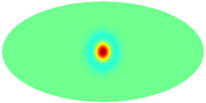
(a) Spherical Mexican hat wavelet (SMHW)

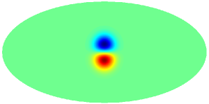
(b) Spherical butterfly wavelet (SBW)

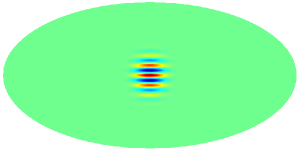
(c) Spherical real Morlet wavelet (SMW)

Figure 2: Spherical wavelets at scale $a=b=0.2$. Wavelet maps are displayed in the Mollweide projection, where the wavelets have been rotated down from the north pole for ease of observation. The SMW is plotted for wave vector $\mathbf{k}=(10,0)^{T}$.

A full directional wavelet analysis on the unit sphere for large data sets has previously been prohibited by the computational infeasibility of any implementation. The computational burden of computing many orientations may be reduced by using steerable wavelets, for which any continuous orientation can be computed from a small number of basis orientations [27]. This is achieved since steerable wavelets have a limited azimuthal band limit and may thus be represented as a finite sum of trigonometric exponentials [27]. However, in this case one must still compute the initial transform for more than one orientation, so although the computational burden is reduced, it is still significant. Moreover, we also require a fast approach for general non-steerable, directional wavelets. We address this problem in the following section by presenting a fast algorithm to perform the directional CSWT.

III Algorithms

A range of algorithms of varying computational efficiency and numerical accuracy are presented to perform the CSWT described in section II. We implement these algorithms in Fortran 90 and subsequently compare computational complexity and typical execution time. The synthesis of a signal from its wavelet coefficients is not considered any further. Without loss of generality we consider only a single dilation (i.e. fixed $a$ and $b$).

III-A Tessellation schemes

It is necessary to discretise both the spherical coordinates of a function defined on the unit sphere and also the Euler angle representation of the $\mathrm{SO}(3)$ rotation group. The fast algorithms we present are performed in harmonic space and hence are tessellation independent, provided an appropriate spherical harmonic transform is defined for the tessellation. However, the semi-fast algorithm is restricted to an equi-angular tessellation of the sphere. The various tessellation schemes adopted are defined below.

The equi-angular tessellation (also known as the equidistant cylindrical projection (ECP)) of the spherical coordinates is defined by $\mathcal{C}=\{\theta_{n_{\theta}}=\frac{\pi{n_{\theta}}}{{N_{\theta}}},\,\phi_{n_{\theta}}=\frac{2\pi{n_{\phi}}}{{N_{\phi}}}:0\leq{n_{\theta}}\leq{N_{\theta}}-1,\,0\leq{n_{\phi}}\leq{N_{\phi}}-1\}$. Let ${N_{\rm{pix}}}={N_{\theta}}{N_{\phi}}$ denote the number of pixels in the tessellation.

We also consider the HEALPix tessellation scheme since it is commonly used for astrophysical data-sets of the CMB. Pixels in the HEALPix scheme are of equal area and are located on rings of constant latitude (the latter feature enables fast spherical harmonic transforms on the pixelised grid). We refer the reader to [33] for details of the HEALPix scheme and here just define the HEALPix grid in terms of pixel indices: $\mathcal{H}=\{(\theta,\phi)_{p}=(\theta_{p},\phi_{p}):0\leq{p}\leq{N_{\rm{pix}}}-1\}$. The HEALPix resolution is parameterised by ${N_{\rm{side}}}$, where ${N_{\rm{pix}}}=12{N_{\rm{side}}}^{2}$. It should be noted that an exact quadrature formula does not exist for the HEALPix tessellation, thus spherical harmonic transforms are necessarily approximate. This is not the case for the ECP or other practical tessellations (e.g. IGLOO and GLESP) where exact quadrature may be performed.

The Euler angle domain of the spherical wavelet coefficients is in general arbitrary, however we use the equi-angular discretisation defined by $\mathcal{E}_{1}=\{\alpha_{n_{\alpha}}=\frac{2\pi{n_{\alpha}}}{{N_{\alpha}}},\,\beta_{n_{\beta}}=\frac{\pi{n_{\beta}}}{{N_{\beta}}},\,\gamma_{n_{\gamma}}=\frac{2\pi{n_{\gamma}}}{{N_{\gamma}}}:0\leq{n_{\alpha}}\leq{N_{\alpha}}-1,\,0\leq{n_{\beta}}\leq{N_{\beta}}-1,\,0\leq{n_{\gamma}}\leq{N_{\gamma}}-1\}$. Our fast algorithm, however, requires (for convenience) the tessellation $\mathcal{E}_{2}=\{\alpha_{n_{\alpha}}=\frac{2\pi{n_{\alpha}}}{{N_{\alpha}}},\,\beta_{n_{\beta}}=\frac{2\pi{n_{\beta}}}{{N_{\beta}}},\,\gamma_{n_{\gamma}}=\frac{2\pi{n_{\gamma}}}{{N_{\gamma}}}:0\leq{n_{\alpha}}\leq{N_{\alpha}}-1,\,0\leq{n_{\beta}}\leq 2{N_{\beta}}-1,\,0\leq{n_{\gamma}}\leq{N_{\gamma}}-1\}$, where the $\beta$ sampling is repeated. Evaluating $\beta$ over the range $0$ to $2\pi$ is redundant, covering the $\mathrm{SO}(3)$ manifold exactly twice. Nonetheless, the use of our fast algorithm requires this range. Such an approach is not uncommon, as [40, 41] also oversample a function of the sphere in the $\theta$ direction in order to develop fast spherical harmonic transforms on equi-angular grids. The overhead associated with our inefficient discretisation is more than offset by the fast algorithm it affords, as described in section III-E.

III-B Direct case

The CSWT defined by (8) may be implemented directly by applying an appropriate quadrature rule. Using index subscripts to denote sampled signals, the direct CSWT implementation is given by

$$({W_{\psi}^{s}})_{{n_{\alpha}},{n_{\beta}},{n_{\gamma}}}=$$ (15)

$$\displaystyle\sum_{{p}=0}^{{N_{\rm{pix}}}-1}\left[R\left(\frac{2\pi{n_{\alpha}}}{{N_{\alpha}}},\frac{\pi{n_{\beta}}}{{N_{\beta}}},\frac{2\pi{n_{\gamma}}}{{N_{\gamma}}}\right)\psi\right]_{{p}}^{\ast}s_{{p}}\>w_{p}\>,$$

where the pixel sum is over all the pixels of any chosen tessellation. The weights for the ECP $\mathcal{C}$ grid are given by $w_{p}=w_{{n_{\theta}}}=\frac{2\pi^{2}\sin{\theta_{n_{\theta}}}}{{N_{\theta}}{N_{\phi}}}$, whereas the equal pixel areas of the HEALPix $\mathcal{H}$ grid ensure the pixel weights, given by $w_{p}=\frac{4\pi}{{N_{\rm{pix}}}}$, are independent of position.

Discretisation techniques other than the plain Riemann sum used in (15) would be beneficial only if additional regularity conditions are imposed on the signal $s$ [23]. It is also possible to choose other weights to achieve a better approximation of the integral. An example of a different equi-angular discretisation and a different choice for the weights is given by the sampling theorem for band-limited functions on the sphere developed by [41].

Evaluation of (15) requires the computation of a 2-dimensional summation, evaluated over a 3-dimensional grid. We assume the number of samples for each discretised angle, except $\gamma$, is of the same order ${N}$. Typically the number of samples in the $\gamma$ direction is of a much lower order, so we treat this term separately. The complexity of the direct algorithm is $\mathcal{O}({N_{\gamma}}{N}^{4})$.

III-C Semi-fast case

We rederive here the semi-fast implementation of the CSWT described by [23] and implemented using the YAWTb Matlab wavelet toolbox and SpharmonicKit. This algorithm involves performing a separation of variables so that one rotation may be performed in Fourier space. The algorithm is restricted to the equi-angular grid $\mathcal{C}$ (in essence pixels must only be defined on equal latitude rings, however some form of interpolation and down-sampling is then required to extract samples for equal longitudes).

Firstly, the $\alpha$ rotation is represented by shifting the corresponding wavelet samples to give

$$({W_{\psi}^{s}})_{{n_{\alpha}},{n_{\beta}},{n_{\gamma}}}=$$

$$\displaystyle\sum_{{n_{\theta}}=0}^{{N_{\theta}}-1}\sum_{{n_{\phi}}=0}^{{N_{\phi}}-1}\left[R\left(0,\frac{\pi{n_{\beta}}}{{N_{\beta}}},\frac{2\pi{n_{\gamma}}}{{N_{\gamma}}}\right)\psi\right]_{{n_{\theta}},{n_{\phi}}-{n_{\alpha}}}^{\ast}\!\!s_{{n_{\theta}},{n_{\phi}}}w_{n_{\theta}}\>,$$

where the index ${n_{\phi}}$ is extended periodically with period ${N_{\phi}}$. The discrete space convolution theorem may then be applied to represent the inner summation as the inverse discrete Fourier transform (DFT) of the product of the wavelet and signal DFT samples (note that only a 1-dimensional DFT is performed in the azimuthal direction):

$$({W_{\psi}^{s}})_{{n_{\alpha}},{n_{\beta}},{n_{\gamma}}}=$$ (16)

$$\sum_{{n_{\theta}}=0}^{{N_{\theta}}-1}\left\{\frac{1}{{N_{\phi}}}\right.\sum_{{k}=0}^{{N_{\phi}}-1}\mathcal{F}^{\ast}\left[R\left(0,\frac{\pi{n_{\beta}}}{{N_{\beta}}},\frac{2\pi{n_{\gamma}}}{{N_{\gamma}}}\right)\psi\right]_{{n_{\theta}},{k}}$$

$$\left.\times\>{\mathcal{F}(s)}_{{n_{\theta}},{k}}\>e^{\frac{\mathit{i}2\pi{k}{n_{\phi}}}{{N_{\phi}}}}\right\}w_{n_{\theta}}\>,$$

where $\mathcal{F}(\cdot)_{n,k}$ denotes 1-dimensional DFT coefficients. A fast Fourier transform (FFT) may then be applied to evaluate simultaneously all of the ${n_{\alpha}}$ terms of the expression enclosed in the curly braces in (16). A final summation (integral) over ${n_{\theta}}$ produces the spherical wavelet coefficients for a given ${n_{\beta}}$ and ${n_{\gamma}}$, for all ${n_{\alpha}}$. Applying an FFT to evaluate simultaneously one summation rapidly, reduces the complexity of the CSWT implementation to $\mathcal{O}({N_{\gamma}}{N}^{3}\log_{2}{N})$.

III-D Fast azimuthally symmetric case

The fast azimuthally symmetric CSWT algorithm is posed in harmonic space, where $\widehat{s}_{\ell m}=\left<Y_{\ell m}\mid s\right>$ are the spherical harmonic coefficients of a function $s\in L^{2}({S^{2}},\mathrm{\,d}\Omega)$, as described in section II-C. For the special case where the wavelet is azimuthally symmetric (i.e. invariant under azimuthal rotations), it is essentially only a function of $\theta$ and may be represented in terms of its Legendre expansion. In this case the harmonic representation of the wavelet coefficients is given by the product of the signal and wavelet spherical harmonic coefficients:

$$(\widehat{{W_{\psi}^{s}}})_{\ell m}=\sqrt{\frac{4\pi}{2\ell+1}}\>\widehat{\psi}_{\ell 0}^{\ast}\>\widehat{s}_{\ell m}\>,$$ (17)

noting that the harmonic coefficients of an azimuthally symmetric wavelet are zero for $m\neq 0$. In practice, one requires that at least one of the signals, usually the wavelet, has a finite band limit so that negligible power is present in those coefficients above a certain ${\ell_{\rm max}}$. We then only need to consider $\ell\leq{\ell_{\rm max}}$ (a detailed discussion of the determination of ${\ell_{\rm max}}$ is presented in [25]). Once the spherical harmonic representation of the wavelet coefficients is calculated by (17), the inverse spherical harmonic transform is applied to compute the wavelet coefficients in the Euler domain. The complexity of the fast isotropic CSWT algorithm is dominated by the spherical harmonic transforms. For a tessellation containing pixels on rings of constant latitude, a fast spherical harmonic transform may be performed (see e.g.[42, 43, 33]). This reduces the complexity of the spherical harmonic transform from $\mathcal{O}({N}^{4})$ to $\mathcal{O}({N}^{3})=\mathcal{O}({N_{\rm{pix}}}^{3/2})$. For certain tessellation schemes fast spherical harmonic transforms of lower complexity are also available, however these are related directly to the tessellation (e.g. [42, 43, 40, 41]). In particular, the algorithm developed by [40, 41] for the ECP tessellation scales as $\mathcal{O}({N}^{2}\log{N})$.

The fast azimuthally symmetric CSWT algorithm is posed purely in harmonic space and consequently the algorithm is tessellation independent. However, we are restricted to azimuthally symmetric wavelets and lose the ability to perform the directional analysis inherent in the wavelet transform construction.

III-E Fast directional case

We present the most general fast directional CSWT algorithm for non-azimuthally symmetric wavelets, i.e. steerable and directional wavelets, in this section. Again, the algorithm is posed purely in harmonic space and so is tessellation independent. We do, however, use the equi-angular $\mathcal{E}_{2}$ discretisation of the wavelet coefficient domain, although other discretisations may be used if FFTs are also defined on these grids. The CSWT at a particular scale (i.e. a particular $a$ and $b$) is essentially a spherical convolution, hence we apply the fast spherical convolution algorithm proposed by [35] to evaluate the wavelet transform. The algorithm proceeds by factoring the rotation into two separate rotations, each of which involves only a constant polar rotation component. Azimuthal rotations may then be performed in harmonic space at far less computation expense than polar rotations. We subsequently rederive the fast spherical convolution algorithm developed by [35], as applied to our application of evaluating the CSWT. The harmonic representation of the CSWT is first presented, followed by the discretisation and fast implementation.

III-E1 Harmonic formulation

Substituting the spherical harmonic expansions of the wavelet and signal into the wavelet transform defined by (8), and noting the orthogonality of the spherical harmonics described by (11), yields the harmonic representation

$${W_{\psi}^{s}}(\alpha,\beta,\gamma)=$$ (18)

$$\sum_{\ell=0}^{{\ell_{\rm max}}}\>\sum_{m=-\ell}^{\ell}\>\sum_{m^{\prime}=-\ell}^{\ell}\left[{D_{mm^{\prime}}^{\ell}(\alpha,\beta,\gamma)\,\widehat{\psi}_{\ell m^{\prime}}}\right]^{\ast}\widehat{s}_{\ell m}\>.$$

Again, we assume negligible power above ${\ell_{\rm max}}$ in at least one of the signals, usually the wavelet, so that the outer summation is truncated to ${\ell_{\rm max}}$. The additional summation over $m^{\prime}$ and the $D_{mm^{\prime}}^{\ell}$ Wigner rotation matrices that are introduced characterise the rotation of a spherical harmonic, noting that a rotated spherical harmonic may be represented by a sum of harmonics of the same $\ell$ [44, 11]:

$$\left[R(\alpha,\beta,\gamma)Y_{{\ell m}}\right](\omega)=\sum_{m^{\prime}=-\ell}^{\ell}D_{m^{\prime}m}^{\ell}(\alpha,\beta,\gamma)\>Y_{\ell m^{\prime}}(\omega)\>.$$

The Wigner rotation matrices may be decomposed as [44, 11]

$$D_{mm^{\prime}}^{\ell}(\alpha,\beta,\gamma)=e^{-\mathit{i}m\alpha}\>d_{mm^{\prime}}^{\ell}(\beta)\>e^{-\mathit{i}m^{\prime}\gamma}\>,$$ (19)

where the real polar $d$-matrix is defined by [44]

$$d^{\ell}_{mm^{\prime}}(\beta)=\sum_{t=\max(0,m-m^{\prime})}^{\min(\ell+m,\ell-m^{\prime})}(-1)^{t}$$

$$\times\frac{\left[(\ell+m)!\,(\ell-m)!\,(\ell+m^{\prime})!\,(\ell-m^{\prime})!\,\right]^{1/2}}{(\ell+m-t)!\,(\ell-m^{\prime}-t)!\,(t+m^{\prime}-m)!\,t!}$$

$$\times\left[\cos\!\left(\frac{\beta}{2}\right)\right]^{2\ell+m-m^{\prime}-2t}\left[\sin\!\left(\frac{\beta}{2}\right)\right]^{m^{\prime}-m+2t}\>,$$

and the sum over $t$ is defined so that the arguments of the factorials are non-negative. Recursion formulae are available to compute rapidly the Wigner rotation matrices in the basis of either complex [45, 10] or real [46, 47] spherical harmonics. We employ the recursion formulae described in [45] in our implementation. The decomposition shown in (19) is exploited by factoring the rotation $R(\alpha,\beta,\gamma)$ into two separate rotations, both of which only contain a constant $\pm\pi/2$ polar rotation:

$$R(\alpha,\beta,\gamma) = R(\alpha-\pi/2,\;-\pi/2,\;\beta)$$ (20)

$$\times\>R(0,\;\pi/2,\;\gamma+\pi/2)\>.$$

By factoring the rotation in this manner and applying the decomposition described by (19), (18) can be rewritten as

$${W_{\psi}^{s}}(\alpha,\beta,\gamma)=$$ (21)

$$\sum_{\ell=0}^{{\ell_{\rm max}}}\>\sum_{m=-\ell}^{\ell}\>\sum_{m^{\prime}=-\ell}^{\ell}\sum_{m^{\prime\prime}=-\min(m_{\rm max},\ell)}^{\min(m_{\rm max},\ell)}d_{m^{\prime}m}^{\ell}(\pi/2)\>$$

$$\times\>d_{m^{\prime}m^{\prime\prime}}^{\ell}(\pi/2)\>\widehat{\psi}_{\ell m^{\prime\prime}}^{\ast}\>\widehat{s}_{\ell m}$$

$$\times\>e^{\mathit{i}[m(\alpha-\pi/2)+m^{\prime}\beta+m^{\prime\prime}(\gamma+\pi/2)]}\>,$$

where the symmetry relationship $d_{mm^{\prime}}^{\ell}(-\beta)=d_{m^{\prime}m}^{\ell}(\beta)$ has been applied. (A similar factoring of the rotation and harmonic space representation has been independently performed in [48].) Steerable wavelets may have a low effective band limit $m_{\rm max}\ll{\ell_{\rm max}}$, in which case the the inner summation in (21) may be truncated to $m_{\rm max}$. For general directional wavelets this is not the case and one must use $m_{\rm max}={\ell_{\rm max}}$.

Evaluating the harmonic formulation given by (21) directly would be no more efficient that approximating the initial integral (8) using simple quadrature. However, (21) is represented in such a way that the presence of complex exponentials may be exploited such that FFTs may be applied to evaluate rapidly the three summations simultaneously.

III-E2 Fast implementation

Azimuthal rotations may be applied with far less computational expense than polar rotations since they appear within complex exponentials in (21). Although the $d$-matrices can be evaluated reasonably quickly and reliably using recursion formulae, the basis for the fast implementation is to avoid these polar rotations as much as possible and use FFTs to evaluate rapidly all of the azimuthal rotations simultaneously. This is the motivation for factoring the rotation by (20) so that all Euler angles occur as azimuthal rotations.

The discretisation of each Euler angle may in general be arbitrary. However, to exploit standard FFT routines uniform sampling is adopted, i.e. grid $\mathcal{E}_{2}$ is used (see section III-A). As mentioned, this discretisation is inefficient since it covers the $\mathrm{SO}(3)$ manifold exactly twice, nevertheless it enables the use of standard FFT routines which significantly increases the speed of the algorithm. Discretising (21) in this manner and interchanging the order of summation we obtain

$$({W_{\psi}^{s}})_{{n_{\alpha}},{n_{\beta}},{n_{\gamma}}}=$$

$$\displaystyle\sum_{m=-{\ell_{\rm max}}}^{{\ell_{\rm max}}}\>\sum_{m^{\prime}=-{\ell_{\rm max}}}^{{\ell_{\rm max}}}\>\sum_{m^{\prime\prime}=-m_{\rm max}}^{m_{\rm max}}$$

$$\displaystyle\sum_{\ell=\max(\mid m\mid,\mid m^{\prime}\mid,\mid m^{\prime\prime}\mid)}^{{\ell_{\rm max}}}d_{m^{\prime}m}^{\ell}(\pi/2)\>d_{m^{\prime}m^{\prime\prime}}^{\ell}(\pi/2)\>\widehat{\psi}_{{\ell m}^{\prime\prime}}^{\ast}\>\widehat{s}_{{\ell m}}$$

$$\times\>e^{\mathit{i}[m(2\pi{n_{\alpha}}/{N_{\alpha}}-\pi/2)+m^{\prime}2\pi{n_{\beta}}/{N_{\beta}}+m^{\prime\prime}(2\pi{n_{\gamma}}/{N_{\gamma}}+\pi/2)]}\>.$$

Shifting the indices yields

$$({W_{\psi}^{s}})_{{n_{\alpha}},{n_{\beta}},{n_{\gamma}}}=$$ (22)

$$\displaystyle\sum_{m=0}^{2{\ell_{\rm max}}}\>\sum_{m^{\prime}=0}^{2{\ell_{\rm max}}}\>\sum_{m^{\prime\prime}=0}^{2m_{\rm max}}e^{\mathit{i}2\pi({n_{\alpha}}m/{N_{\alpha}}+{n_{\beta}}m^{\prime}/{N_{\beta}}+{n_{\gamma}}m^{\prime\prime}/{N_{\gamma}})}$$

$$\times\>T_{m,m^{\prime},m^{\prime\prime}}\>,$$

where

$$T_{m,m^{\prime},m^{\prime\prime}}=e^{\mathit{i}(m^{\prime\prime}-m)\pi/2}$$ (23)

$$\times\displaystyle\sum_{\ell=\max(\mid m\mid,\mid m^{\prime}\mid,\mid m^{\prime\prime}\mid)}^{{\ell_{\rm max}}}d_{m^{\prime}m}^{\ell}(\pi/2)\>d_{m^{\prime}m^{\prime\prime}}^{\ell}(\pi/2)$$

$$\times\>\widehat{\psi}_{\ell m^{\prime\prime}}^{\ast}\>\widehat{s}_{\ell m}$$

is extended periodically. Note that the phase shift introduced by shifting the indices of the summation in (22), shifts the $T_{m,m^{\prime},m^{\prime\prime}}$ indices back. Making the associations ${N_{\alpha}}=2{\ell_{\rm max}}+1$, ${N_{\beta}}=2{\ell_{\rm max}}+1$ and ${N_{\gamma}}=2m_{\rm max}+1$, one notices that (22) is the unnormalised 3-dimensional inverse DFT of (23). Nyquist sampling in $(\alpha,\beta,\gamma)$ is inherently ensured by the associations made with ${\ell_{\rm max}}$ and $m_{\rm max}$.

The CSWT may be performed rapidly in spherical harmonic space by constructing the $T$-matrix of (23) from spherical harmonic coefficients and precomputed $d$-matrices, followed by the application of an FFT to evaluate rapidly all three Euler angles of the discretised CSWT simultaneously. The complexity of the algorithm is dominated by the computation of the $T$-matrix. This involves performing a 1-dimensional summation over a 3-dimensional grid, hence the algorithm is of order $\mathcal{O}({N_{\gamma}}{N}^{3})$.

Additional benefits may be realised for real signals by exploiting the resulting conjugate symmetry relationship. Memory and computational requirements may be reduced by a further factor of two for real signals by noting the conjugate symmetry relationship $T_{-m,-m^{\prime},-m^{\prime\prime}}=T_{m,m^{\prime},m^{\prime\prime}}^{\ast}$. In our implementation we use the complex-to-real FFT routines of the FFTW package, which are approximately twice as fast as the equivalent complex-to-complex routines.

III-F Comparison

We summarise the computational complexities of the various CSWT algorithms for a single pair of scales and single orientation in Table I. The complexity of each algorithm scales with the number of dilations considered and, for those algorithms that facilitate a directional analysis (i.e. all but the fast azimuthally symmetric algorithm), with the number of orientations considered. The most general fast directional algorithm provides a saving of $\mathcal{O}({N})$ over the direct case, where the number of pixels on the sphere and the harmonic band limit are related to ${N}$ by $\mathcal{O}({N_{\rm{pix}}})=\mathcal{O}({\ell_{\rm max}}^{2})=\mathcal{O}({N}^{2})$.

TABLE I: Algorithm complexity for one scale and one orientation.

Algorithm	Complexity
Direct	$\mathcal{O}({N}^{4})$
Semi-fast	$\mathcal{O}({N}^{3}\log_{2}{N})$
Fast azimuthally symmetric	$\mathcal{O}({N}^{3})$
Fast directional	$\mathcal{O}({N}^{3})$

We implement all algorithms in Fortran 90, adopting the HEALPix tessellation of the sphere (which, incidentally, is the tessellation scheme of the WMAP CMB data [2]). Typical execution times for the algorithms are tabulated in Table II for a range of resolutions from 110 down to 3.4 arcminutes. The improvements provided by the fast algorithms are apparent. Indeed, it is not feasible to run the direct algorithm on data-sets with a resolution much greater than ${N_{\rm{pix}}}\simeq 5\times 10^{5}$. For data-sets of practical size, such as the WMAP (${N_{\rm{pix}}}\simeq 3\times 10^{6}$) and forthcoming Planck (${N_{\rm{pix}}}\simeq 50\times 10^{6}$) CMB data, the fast implementations of the CSWT are essential.

The semi-fast algorithm is also implemented using the HEALPix tessellation. However, to perform the outer summation (integration) continual interpolation followed by down-sampling is required on each iso-latitude ring to essentially resample the data on an ECP tessellation. This increases the execution time of the implementation of the semi-fast algorithm on the HEALPix grid to an extent that the semi-fast algorithm provides little advantage over the direct algorithm. To appreciate the advantages of the semi-fast approach it must be implemented on an ECP tessellation, hence we do not tabulate the execution times for our implementation of this algorithm on the HEALPix grid as it provides an unfair comparison.

It is also important to note that although complexity scales with the number of dilations and orientations considered, execution time does not for the fast algorithms. Execution time does scale in this manner for the direct algorithm. There are a number of additional overheads associated with the fast algorithms, such as computing spherical harmonic coefficients and $d$-matrices. Consequently, the fast algorithms provide additional execution time savings that are not directly apparent in Table II. For example, the execution time of the fast azimuthally symmetric and directional algorithms for 10 dilations at a resolution of ${N_{\rm{pix}}}\simeq 8\times 10^{5}$ (${N_{\rm{side}}}=256$) are 3:08.20 and 7:06.83 (minutes:seconds) respectively, which is considerably faster than ten times the execution time of one dilation.

TABLE II: Typical execution time (minutes:seconds) for each algorithm run on an Intel P4-M 3GHz laptop with 512MB of memory.

Resolution		Algorithm execution time
${N_{\rm{side}}}$	${N_{\rm{pix}}}$	Direct	Fast isotropic	Fast directional
32	12,288	3:25.37	0:00.06	0:00.10
64	49,152	54:31.75	0:00.38	0:00.74
256	786,432	–	0:28.00	0:52.55
512	3,257,292	–	3:43.69	7:57.75
1024	12,582,912	–	28:23.85	71:31.68

IV Application

We demonstrate in this section the application of our CSWT implementation to binary Earth data. In Fig. 3 the Earth data and the corresponding spherical wavelet coefficients are shown. We use the SBW defined in section II-D to perform the analysis. This is a steerable wavelet [27], however our implementation is in general valid for any directional wavelet. Notice how the wavelet coefficient maps corresponding to different oriented wavelets pick out corresponding oriented structure in the data. As the dilation scale is increased, the scale of the features extracted also increases accordingly.

The ability to probe oriented structure in data defined on a sphere is of important practical use. Certain physical processes may be localised on the sphere in scale, position and orientation (e.g. signatures of cosmic strings in the CMB [49] or correlations induced in the CMB by the nearby galaxy distribution [50]). Thus, analysing the statistical properties of spherical wavelet coefficients individually for a range of scales, positions and orientations may allow one to detect such effects with greater significance. Indeed, using a directional spherical wavelet analysis we have made very strong detections of non-Gaussianity in the CMB [36, 37] and the strongest detection made to date of the ISW effect [38].

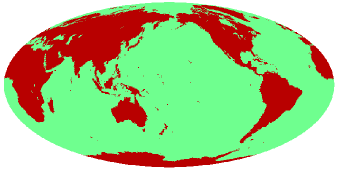
(a) Binary Earth map

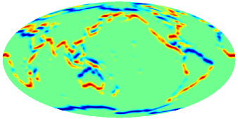
(b) Spherical butterfly wavelet coefficients for scale $a=b=0.03$ and orientation $\gamma=0^{\circ}$

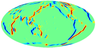
(c) Spherical butterfly wavelet coefficients for scale $a=b=0.03$ and orientation $\gamma=144^{\circ}$

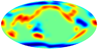
(d) Spherical butterfly wavelet coefficients for scale $a=b=0.12$ and orientation $\gamma=0^{\circ}$

(e) Spherical butterfly wavelet coefficients for scale $a=b=0.12$ and orientation $\gamma=144^{\circ}$

Figure 3: Binary Earth data and corresponding spherical butterfly wavelet coefficients. The wavelet coefficients for combinations of only two scales and two orientations are shown. Notice how the wavelet coefficient maps corresponding to different oriented wavelets pick out corresponding oriented structure in the data. As the dilation scale is increased, the scale of the features extracted also increases accordingly. Directional wavelets therefore allow one not only to probe signal characteristics localised in scale and space, but also in orientation. However, the concept of orientation on the sphere is necessarily a local one (see text section II-C for further details).

V Concluding remarks

The extension of Euclidean wavelet analysis to the sphere has been described in the framework presented by [27], where the stereographic projection is used to relate the spherical and Euclidean constructions. We extend the concept of the spherical dilation presented by [27] to anisotropic dilations. Although anisotropic dilations are of practical use, the resulting basis one projects onto does not classify as a wavelet basis since perfect reconstruction is not possible.

Current and forthcoming data-sets on the sphere, of the CMB for example, are of considerable size as higher resolutions are necessary to test new physics. Consequently, we present fast algorithms to implement the CSWT as an analysis without such algorithms is not computationally feasible. A range of algorithms are described, from the direct quadrature approximation, to the semi-fast equi-angular algorithm where one rotation is performed in Fourier space, to the fast azimuthally symmetric and directional algorithms posed purely in spherical harmonic space. Posing the CSWT purely in harmonic space naturally ensures the resulting algorithms are tessellation independent. The most general fast directional algorithm provides a saving of $\mathcal{O}(\sqrt{{N_{\rm{pix}}}})=\mathcal{O}({\ell_{\rm max}})$ over the direct implementation and may be performed down to a few arcminutes even with limited computational resources.

Data is observed on a sphere in a range of applications. In many of these cases the ability to perform a wavelet analysis would be useful. For example, spherical wavelets may be used to probe the CMB for deviations from the standard assumption of Gaussianity, or to search for compact objects embedded in the CMB, such as cosmic strings, a predicted but as yet unobserved phenomenon. The extension of wavelet analysis to the sphere enables one to probe new physics in many areas, and is facilitated on large practical data-sets by our fast directional CSWT algorithm.

Jason McEwen was born in Wellington, New Zealand, in August 1979. He received a B.E. (Hons) degree in Electrical and Computer Engineering from the University of Canterbury, New Zealand, in 2002. Currently, he is working towards a Ph.D. degree at the Astrophysics Group, Cavendish Laboratory, Cambridge. His area of interests include spherical wavelets and the cosmic microwave background.

Michael Hobson was born in Birmingham, England, in September 1967. He received the B.A. degree in natural sciences with honours and the Ph.D. degree in astrophysics from the University of Cambridge, England, in 1989 and 1993 respectively. Since 1993, he has been a member of the Astrophysics Group of the Cavendish Laboratory at the University of Cambridge, where he has been a Reader in Astrophysics and Cosmology since 2003. His research interests include theoretical and observational cosmology, particularly anisotropies in the cosmic microwave background, gravitation, Bayesian analysis techniques and theoretical optics.

Daniel Mortlock was born in Melbourne, Australia, in June 1973. He received the B.Sc. and Ph.D. degrees in science from The University of Melbourne, Melbourne, Australia, in 1994 and 2000, respectively. From 1999 to 2002 he was research associate at The Cavendish Laboratory, Cambridge, UK. In 2002 he moved to The Institute of Astronomy, Cambridge, UK as a postdoctoral fellow. His research interests include cosmology, gravitational lensing and statistical analysis of large data-sets.

Anthony Lasenby was born in Malvern, England, in June 1954. He received a B.A. then M.A. from the University of Cambridge in 1975 and 1979, an M.Sc. from Queen Mary College, London in 1978 and a Ph.D. from the University of Manchester in 1981. His Ph.D. work was carried out at the Jodrell Bank Radio Observatory specializing in the Cosmic Microwave Background, which has been a major subject of his research ever since. After a brief period at the National Radio Astronomy Observatory in America, he moved from Manchester to Cambridge in 1984, and has been at the Cavendish Laboratory Cambridge since then. He is currently Head of the Astrophysics Group and the Mullard Radio Astronomy Observatory in the Cavendish Laboratory, and a Deputy Head of the Laboratory. His other main interests include theoretical physics and cosmology, the application of new geometric techniques in computer graphics and electromagnetic modelling, and statistical techniques in data analysis.

References

- [1] C. L. Bennett, A. Banday, K. M. Gorski, G. Hinshaw, P. Jackson, P. Keegstra, A. Kogut, G. F. Smoot, D. T. Wilkinson, and E. L. Wright, “4-year COBE DMR cosmic microwave background observations: Maps and basic results,” Astrophys. J. Lett., vol. 464, no. 1, pp. 1–4, 1996.
- [2] C. L. Bennett, M. Halpern, G. Hinshaw, N. Jarosik, A. Kogut, M. Limon, S. S. Meyer, L. Page, D. N. Spergel, G. S. Tucker, E. Wollack, E. L. Wright, C. Barnes, M. R. Greason, R. S. Hill, E. Komatsu, M. R. Nolta, N. Odegard, H. V. Peiris, L. Verde, and J. L. Weiland, “First-year Wilkinson Microwave Anisotropy Probe (WMAP) observations: Preliminary maps and basic results,” Astrophys. J. Supp., vol. 148, no. 1, pp. 1–28, 2003.
- [3] M. A. Wieczorek, “Gravity and topology of terrestrial planets,” submitted to Treatise on Geophysics, 2006.
- [4] M. A. Wieczorek and R. J. Phillips, “Potential anomalies on a sphere: Applications to the thickness of the lunar crust,” J. Geophys. Res., vol. 103, pp. 383–395, 1998.
- [5] D. L. Turcotte, R. J. Willemann, W. F. Haxby, and J. Norberry, “Role of membrane stresses in the support of planetary topology,” J. Geophys. Res., vol. 86, pp. 3951–3959, 1981.
- [6] K. A. Whaler, “Downward continuation of Magsat lithosphere anomalies to the Earth’s surface,” Geophys. J. R. astr. Soc., vol. 116, pp. 267–278, 1994.
- [7] S. Swenson and J. Wahr, “Methods for inferring regional surface-mass anomalies from GRACE measurements of time-variable gravity,” J. Geophys. Res., vol. 107, pp. 2193–278, 2002.
- [8] F. J. Simons, F. A. Dahlen, and M. A. Wieczorek, “Spatiospectral concentration on a sphere,” SIAM Rev., p. in press, 2006.
- [9] R. Ramamoorthi and P. Hanrahan, “A signal processing framework for reflection,” ACM Transactions on Graphics, vol. 23, no. 4, pp. 1004–1042, 2004.
- [10] C. H. Choi, J. Ivanic, M. S. Gordon, and K. Ruedenberg, “Rapid and stable determination of rotation matrices between spherical harmonics by direct recursion,” J. Chem. Phys., vol. 111, no. 19, pp. 8825–8831, 1999.
- [11] D. W. Ritchie and G. J. L. Kemp, “Fast computation, rotation and comparison of low resolution spherical harmonic molecular surfaces,” J. Comput. Chem., vol. 20, no. 4, pp. 383–395, 1999.
- [12] P. Schröder and W. Sweldens, “Spherical wavelets: Efficiently representing functions on the sphere,” in Computer Graphics Proceedings (SIGGRAPH ‘95), 1995, pp. 161–172.
- [13] W. Sweldens, “The lifting scheme: a custom-design constriction of biorthogonal wavelets,” Applied Comput. Harm. Anal., vol. 3, no. 2, pp. 186–200, 1996.
- [14] F. J. Narcowich and J. D. Ward, “Non-stationary wavelets on the m-sphere for scattered data,” Applied Comput. Harm. Anal., vol. 3, pp. 324–336, 1996.
- [15] D. Potts, G. Steidl, and M. Tasche, “Kernels of spherical harmonics and spherical frames,” in Advanced Topic in Multivariate Approximation, F. Fontanella, K. Jetter, and P.-J. Laurent, Eds. Singapore: World Scientific, 1996, pp. 1–154.
- [16] W. Freeden and U. Windheuser, “Combined spherical harmonic and wavelet expansion – a future concept in the Earth’s gravitational determination,” Applied Comput. Harm. Anal., vol. 4, pp. 1–37, 1997.
- [17] W. Freeden, T. Gervens, and M. Schreiner, Constructive approximation on the sphere – with application to geomathematics. Clarendon Press, Oxford, 1997.
- [18] B. Torrésani, “Position-frequency analysis for signals defined on spheres,” Signal Proc., vol. 43, pp. 341–346, 1995.
- [19] S. Dahlke and P. Maass, “Continuous wavelet transforms with applications to analyzing functions on sphere,” J. Fourier Anal. and Appl., vol. 2, pp. 379–396, 1996.
- [20] M. Holschneider, “Continuous wavelet transforms on the sphere,” J. Math. Phys., vol. 37, pp. 4156–4165, 1996.
- [21] J.-P. Antoine and P. Vandergheynst, “Wavelets on the 2-sphere : A group theoretical approach,” Applied Comput. Harm. Anal., vol. 7, pp. 1–30, 1999.
- [22] ——, “Wavelets on the n-sphere and related manifolds,” J. Math. Phys., vol. 39, no. 8, pp. 3987–4008, 1998.
- [23] J.-P. Antoine, L. Demanet, L. Jacques, and P. Vandergheynst, “Wavelets on the sphere: Implementation and approximations,” Applied Comput. Harm. Anal., vol. 13, no. 3, pp. 177–200, 2002.
- [24] J.-P. Antoine, R. Murenzi, P. Vandergheynst, and S. T. Ali, Two-dimensional wavelets and their relatives. Cambridge: Cambridge University Press, 2004.
- [25] I. Bogdanova, P. Vandergheynst, J.-P. Antoine, L. Jacques, and M. Morvidone, “Stereographic wavelet frames on the sphere,” Applied Comput. Harm. Anal., vol. 19, no. 2, pp. 223–252, 2005.
- [26] L. Demanet and P. Vandergheynst, “Gabor wavelets on the sphere,” in SPIE, 2003.
- [27] Y. Wiaux, L. Jacques, , and P. Vandergheynst, “Correspondence principle between spherical and Euclidean wavelets,” Astrophys. J., vol. 632, no. 1, pp. 15–28, 2005.
- [28] H. N. Mhasker, F. J. Narcowich, and J. D. Ward, “Representing and analysing scattered data on spheres,” in Multivariate Approximation and Applications, N. Dyn, D. Leviaton, D. Levin, and A. Pinkus, Eds. Cambridge University Press, 2001.
- [29] E. B. Saff and A. B. J. Kuijlaars, “Distributing many points on a sphere,” Math. Intelligencer, vol. 19, pp. 5–11, 1997.
- [30] D. P. Hardin and E. B. Saff, “Discretizing manifolds via minimum energy points,” Notices of Amer. Math. Soc., vol. 51, no. 10, pp. 1186–1194, 2004.
- [31] Q. Du, M. D. Gunzburger, and I. Ju, “Constrained centroidal voronoi tessellations for surfaces,” SIAM J. Sci. Comput., vol. 24, pp. 1488–1506, 2003.
- [32] R. G. Crittenden and N. G. Turok, “Exactly azimuthal pixelizations of the sky,” preprint (astro-ph/9806374), 1998.
- [33] K. M. Górski, E. Hivon, A. J. Banday, B. D. Wandelt, F. K. Hansen, M. Reinecke, and M. Bartelmann, “Healpix – a framework for high resolution discretization and fast analysis of data distributed on the sphere,” Astrophys. J., vol. 622, pp. 759–771, 2005.
- [34] A. G. Doroshkevich, P. D. Naselsky, O. V. Verkhodanov, D. I. Novikov, V. I. Turchaninov, I. D. Novikov, P. R. Christensen, and L. Y. Chiang, “Gauss–Legendre Sky Pixelization (GLESP) for CMB maps,” Int. J. Mod. Phys. D., vol. 14, no. 2, pp. 275–290, 2005.
- [35] B. D. Wandelt and K. M. Górski, “Fast convolution on the sphere,” Phys. Rev. D., vol. 63, no. 123002, pp. 1–6, 2001.
- [36] J. D. McEwen, M. P. Hobson, A. N. Lasenby, and D. J. Mortlock, “A high-significance detection of non-Gaussianity in the WMAP 1-yr data using directional spherical wavelets,” Mon. Not. Roy. Astr. Soc., vol. 359, pp. 1583–1596, 2005.
- [37] ——, “A high-significance detection of non-Gaussianity in the WMAP 3-yr data using directional spherical wavelets,” submitted to Mon. Not. Roy. Astr. Soc, 2006.
- [38] J. D. McEwen, P. Vielva, M. P. Hobson, E. Martínez-González, and A. N. Lasenby, “Detection of the ISW effect and corresponding dark energy constraints made with directional spherical wavelets,” submitted to Mon. Not. Roy. Astr. Soc, 2006.
- [39] I. Tosic, P. Frossard, and P. Vandergheynst, “Progressive coding of 3D objects based on overcomplete decompositions,” submitted to IEEE Trans. Circuits Syst. Video Technol., 2005.
- [40] J. R. Driscoll and D. M. J. Healy, “Computing Fourier transforms and convolutions on the sphere,” Advances in Applied Mathematics, vol. 15, pp. 202–250, 1994.
- [41] D. M. J. Healy, D. Rockmore, P. J. Kostelec, and S. S. B. Moore, “FFTs for the 2-sphere – improvements and variations,” J. Fourier Anal. and Appl., vol. 9, no. 4, pp. 341–385, 2003.
- [42] M. J. Mohlenkamp, “A fast transform for spherical harmonics,” Ph.D. dissertation, Yale University, Department of Mathematics, 1997.
- [43] ——, “A fast transform for spherical harmonics,” J. Fourier Anal. and Appl., vol. 5, no. 2/3, pp. 159–184, 1999.
- [44] D. M. Brink and G. R. Satchler, Angular Momentum, 3rd ed. Oxford: Clarendon Press, 1993.
- [45] T. Risbo, “Fourier transform summation of Legendre series and d-functions,” J. Geodesy, vol. 70, no. 7, pp. 383–396, 1996.
- [46] J. Ivanic and K. Ruedenberg, “Rotation matrices for real spherical harmonics. Direct determination by recursion,” J. Phys. Chem. A, vol. 100, no. 15, pp. 6342–6347, 1996.
- [47] M. A. Blanco, M. Flórez, and M. Bermejo, “Evaluation of the rotation matrices in the basis of real spherical harmonics,” J. Mol. Struct. (Theochem), vol. 419, pp. 19–27, 1997.
- [48] T. Bulow and K. Daniilidis, “Surface representation using spherical harmoniscs and Gabor wavelets on the sphere,” University of Pennsylvania, Tech. Rep. MS-CIS-01-37, 2001.
- [49] N. Kaiser and A. Stebbins, “Microwave anisotropy due to cosmic strings,” Nature, vol. 310, pp. 391–393, 1984.
- [50] R. G. Crittenden and N. Turok, “Looking for Lambda with the Rees-Sciama effect,” Phys. Rev. Lett., vol. 76, pp. 575–578, 1996.