Fourier Resolved Spectroscopy of the XMM-Newton Observations of MCG -06-30-15

Abstract

We study the Frequency Resolved Spectra of the Seyfert galaxy MCG -06-30-15 obtained during two recent XMM-Newton observations. Splitting the Fourier spectra in soft ($E\mathrel{\raise 1.29167pt\hbox{$<$}\mkern-14.0mu\lower 3.44444pt\hbox{$\sim$}}2$ keV) and hard ($E\mathrel{\raise 2.15277pt\hbox{$>$}\mkern-14.0mu\lower 2.58334pt\hbox{$\sim$}}2$ keV) bands, we find that the soft band has a variability amplitude larger than the hard one on time scales longer than 10 ksec, while the opposite is true on time scales shorter than 3 ksec. Both the soft and hard band spectra are well fitted by power laws of different indices. The spectra of the hard band become clearly softer as the Fourier Frequency decreases from $7\times 10^{-4}$ Hz to $10^{-5}$ Hz, while the spectral slope of the soft band power law component is independent of the Fourier frequency. The well known broad Fe K$\alpha$ feature is absent at all frequency bins; this result implies that this feature is not variable on time scales shorter than $\sim 10^{5}$ sec, in agreement with recent line variability studies. Strong spectral features are also present in the soft X-ray band (at $E\simeq 0.7$), clearly discernible in all Fourier Frequency bins. This fact is consistent with the assumption that they are due to absorption by intervening matter within the source.

1 Introduction

The “standard” picture of the Active Galactic Nuclei (AGN) accretion disk arrangement consists of a geometrically thin, optically thick disk (that produces the quasithermal optical–UV feature known as the “Blue Bump”) supplemented by an overlying, hot ($\sim 10^{8}$ K) corona responsible for the observed X-ray emission. Both these components are presumed to extend to the innermost stable particle orbits associated with the accreting black hole. This latter fact led to the suggestion that studies of the spectral and timing characteristics of these components could provide a probe of the regime of strong gravitational physics.

It has been argued that the reprocessing of X-ray radiation on the much cooler accretion disk would produce a relativistically broadened, asymmetric, Fe K$\alpha$ fluorescence feature at 6.4 keV (Fabian et al.  1989; Stella 1990) and a spectral hardening of the spectrum at energies $E\mathrel{\raise 2.15277pt\hbox{$>$}\mkern-14.0mu\lower 2.58334pt\hbox{$\sim$}}10$ keV due to reflection of the coronal X-rays by neutral matter on the accretion disk surface. It was further argued that the precise shape, EW and variability properties of this feature could allow the mapping of the space–time geometry in the black hole vicinity (Reynolds et al. 1999) and/or the geometric arrangement of the disk and the X-ray emitting plasma (Nayakshin & Kazanas 2001).

AGN observations appear to corroborate these considerations: A broad feature at the correct energy was indeed identified in the ASCA spectra of many AGN (Nandra et al. 1997b). One of the broadest such asymmetric emission features was detected in the energy spectrum of the Seyfert 1 galaxy MCG -06-30-15 (Tanaka et al. 1995). The presence of this emission feature has been confirmed by repeated observations of the source by all recent X-ray missions, including Chandra (Lee et al. 2002) and XMM-Newton (Wilms et al. 2001; Fabian et al. 2002) and thought to suggest, on the basis of its width, the presence of an extreme Kerr geometry for the accreting black hole. At energies below 2 keV MCG -06-30-15 shows great spectral complexity attributed to absorption by partially ionized material and possibly also dust (Turner et al. 2003 and references therein); alternatively, these same features have also been interpreted by some authors due to relativistically broadened soft X-ray emission features (Branduardi-Raymont et al. 2001; Sako et al. 2003).

It should be born in mind though that, however convincing, spectral features by themselves generally provide information only about the properties of the emitting (or absorbing) plasma along the observer’s line of sight, typically just its column density. However, the size or the density of the plasma, parameters needed to determine its dynamics, require additional independent information that, in the absence of sufficient spatial resolution, is provided by the sources’ variability (Kazanas, Hua & Titarchuk 1997). Hence, a more comprehensive approach should involve the use of both spectral and timing information in a combined analysis. A novel approach in this direction has been taken by Revnivtsev, Gilfanov & Churazov (1999) who used the combined RXTE variability - spectral information to produce the energy spectra of Cygnus X-1 in its hard state for different Fourier frequencies. This study showed that the Cyg X-1 spectra depend strongly on the Fourier frequency, with the Fe K$\alpha$ line and the reflection component becoming increasingly visible with decreasing frequency. Very similar results were obtained by the same authors for the Galactic source GX 339-4 (Revnivtsev, Gilfanov & Churazov 2001), while Cyg X-1 in its soft state showed much smaller dependence of its spectrum and Fe K$\alpha$ line on Fourier frequency (Revnivtsev, Gilfanov & Churazov 2000).

In the present paper we apply the method used by Revnivtsev et al. (1999) to MCG -06-30-15. We chose this source because, apart from being considered as the AGN with the archetypal Fe K$\alpha$ profile, it shows large amplitude variations on both short and long time scales (e.g.  McHardy et al. 2005), it is bright in X-rays and has been the target of numerous X-ray observations. Of particular interest amongst them are those by XMM-Newton due to the large area of its instruments, which offer high quality, low noise spectra, albeit at energies less than 10 keV. In §2 and §3 we discuss the data sets and the methodology used and we present our results in the form of energy spectra at three different Fourier frequencies. In §4 our results are discussed briefly in the context of the standard and other models presently in the literature.

2 Data Reduction and Analysis Method

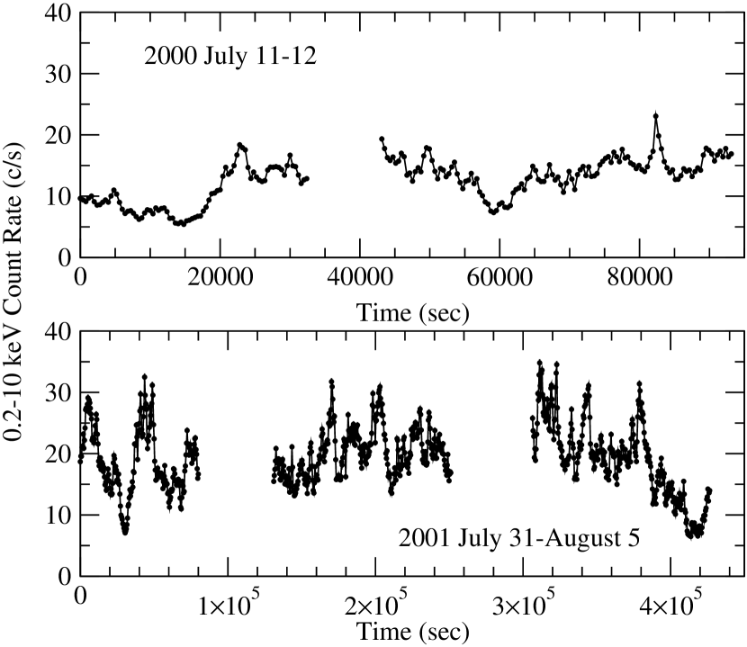
Figure 1: Full-band (0.2-10 keV) EPIC-PN light curves in 400 s bins of both the 2000 and 2001 observations. Errors are plotted, but are very small (typically of the order of $\sim 0.35$ and $0.43$ counts/s,respectively).

MCG -06-30-15 has been observed with XMM-Newton twice. The first observation was performed on 2000 July 10-11 (revolution 108) and the second on 2001 July 31 - August 5 (revolutions 301-303). In this work we use data from the EPIC-PN detector only. In both cases the source was observed on-axis and the PN camera was operated in small window mode, with medium filter applied. We processed the data using SAS v6.0.0. Source data (single and double pixel events, i.e. patterns $0-4$) were extracted from circular regions of radius $40^{\prime\prime}$, and background events from a source free area 2 times larger than the source extraction area. The background was in general low and stable throughout the observations, with the exception of the final few ks of each revolution where the background count rate increases. We kept 83 and 320 ks of “good” exposure time data from the 2000 and 2001 observations, respectively.

Fig. 1 shows the 0.2-10 keV, background subtracted, 400-s binned, EPIC-PN light curves. The source shows large amplitude variations at all time scales. The raw energy spectrum, using data from both observations, is shown in the upper panel of Fig. 2. The energy resolution is significantly reduced for reasons that we explain in the following section. The photon count spectrum is estimated in 22 energy bands only: we consider 6 bands from 0.2 to 0.8 keV with $\Delta E=0.1$ keV, the bands $0.8-1$, $1-1.3$, $1.3-1.6$ and $1.6-2$ keV, 9 bands from 2 to 7 keV with $\Delta E=0.5$ keV, and finally the bands $7-8$ and $8-10$ keV.

The main features are clearly evident even in this low resolution spectrum. The solid line in the upper panel of Fig. 2 shows a power law model spectrum of $\Gamma=2$ and Galactic absorption only ($N_{H}=4.06\times 10^{20}$cm^-2; Elvis, Wilkes, & Lockman 1989). The model normalization is adjusted to produce total number of counts equal to those of the observed spectra (this is the case for the normalization of all model spectra presented in the rest of the paper). In the lower panel of Fig. 2 we show a plot of the data over the model ratio (filled circles). The significantly asymmetric, broad iron line in the energy band $\sim 5-7$ keV and strong residuals in the soft X-ray band can be clearly seen.

2.1 Fourier Resolved Spectroscopy

We now discuss briefly the technique of “Fourier resolved spectroscopy” introduced by Revnivtsev et al. (1999). Suppose we have light curves of a given source at different energy bands $E_{j}$, $j=1,2,\ldots M$. Let us denote with $x(t_{i},E_{j})$ the observed count rate at time $t_{i}$ in the energy band $E_{j}$ ($i=\Delta t,2\Delta t,...,N\Delta t$, $N$ is the total number of points, and $N\Delta t=T$ is the length of the light curve). The power spectrum (PSD) of this light curve can be estimated as follows:

$$P(\nu_{k},E_{j})=\frac{2\Delta t}{N}|a_{k}|^{2},$$ (1)

in units of (counts s${}^{-1})^{2}$ Hz^-1, where $\nu_{k}=k/N\Delta t$ $(k=1,2,...,(N-1)/2)$ and $a_{k}=\sum_{i}x(t_{i},E_{j})e^{i2\pi\nu_{k}t_{i}}$. The finite Fourier representation of the observed time series $x(t_{i},E_{j})$ is equal to the sum of sinusoidal terms (“variability components”) with frequencies $\nu_{k}$. Their amplitudes, $A_{k}$, are related to $|a_{k}|$ through the relation $A_{k}=(2/N)|a_{k}|$. Using equation (1), this relation can be rewritten as follows:

$$A(\nu_{k},E_{j})=\sqrt{\frac{2P(\nu_{k},E_{j})}{N\Delta t}}~{}{\rm counts~{}s}^{-1}.$$ (2)

$A(\nu_{k},E_{j})$, viewed as a function of $E_{j}$, represents the energy spectrum of the component with frequency $\nu_{k}$.

Although MCG -06-30-15 is a bright Seyfert 1 galaxy it is not possible to study its energy dependent variability behavior using the full energy resolution offered by XMM-Newton. Instead, we have split the 0.2-10 keV energy range in the 22 bands referred to in the previous section. These bands were so chosen to: a) be sufficiently broad to yield light curves of reasonably high signal-to-noise for an accurate determination of the power spectrum, and b) their number in the traditional “soft” ($<2$ keV) and “hard” ($>2$ keV) X-ray channels be roughly equal. The two XMM-Newton observations resulted in 5 segments during which the source was observed almost continuously for $T\sim 32-120$ ks (see Fig. 1). For each segment we constructed background-subtracted light curves in the 22 energy bands using a bin size of $\Delta t=100$ s. In this way a total of 105 light curves were produced. We used equation (1) to estimate their power spectrum, after subtracting the associated (constant) Poisson power. In principle, using equation (2), we can now compute the amplitudes $A_{l}(\nu_{k},E_{j}),l=1,\dots,5$. The mean of the five $A_{l}(\nu_{k},E_{j})$ estimates at each $\nu_{k}$, viewed as a a function of $E_{j}$, can constitute the “low-resolution” energy spectrum of the variability components with frequency $\nu_{k}$.

However, the energy spectra of the individual $\nu_{k}$’s turned out to be very noisy. In fact, at high frequencies, after the subtraction of the Poisson noise component, many of the $P(\nu_{k},E_{j})$’s are negative, thus preventing the estimation of the respective $A(\nu_{k},E_{j})$. For this reason, we decided to consider three broad frequency bands : a) $8.3\times 10^{-6}-10^{-4}$ Hz, b) $1-3\times 10^{-4}$ Hz, and c) $3-7\times 10^{-4}$ Hz (hereafter “low/LF”, “medium/MF” and “high-frequency/HF” range, respectively). These frequency bands correspond to time scales of $0.12-1.4$ days, $3-10$ ksec, and $1.5-3$ ksec, respectively. There are $N_{\rm PSD}=39$, 81 and 161 $P(\nu_{k},E_{j})$ estimates in each frequency bin. We computed their mean, $\overline{P(E_{j})}=\sum_{l,k}P(\nu_{k},E_{j})/N_{\rm PSD}$, and used equation (2) to estimate the average amplitude, $\overline{A(E_{j})}$, of the variability components in each frequency band. These values comprise our final estimate of the energy spectrum of the low, medium and high-frequency variability components.

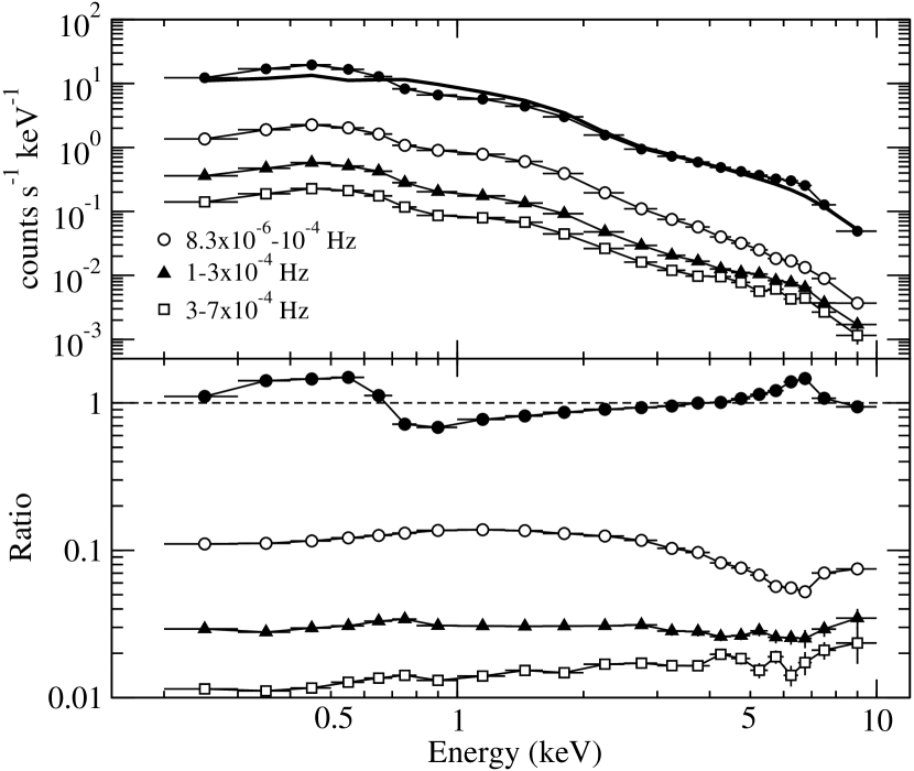
Figure 2: Upper panel: Total EPIC-PN count spectrum (filled circles) and the LF, MF and HF Fourier energy spectra (open circles, filled triangles, and open squares, respectively). The solid line shows a $\Gamma=2$ power law spectrum affected by the Galactic absorption only. Lower panel: Ratio of the total spectrum to the simple power law model (filled circles) and the Fourier resolved spectra normalized to the total EPIC-PN spectrum.

3 Results

The raw, count energy spectra of the LF, MF and HF components (i.e.  $\overline{A(E_{j})}$ divided by $\Delta E$) are also shown in the upper panel of Fig. 2 ( given respectively by the open circles, filled triangles, and open squares). In order to gain some insight into their broad-band shape, we divided them by the raw total energy spectrum of the source. These ratios (shown in the lower panel of Fig. 2) should factor out the broad instrumental response that distorts the spectra and, as a result, should give a better view of their true shape, albeit only in relation to that of our entire data set.

At energies $E<3$ keV the LF and MF normalized spectra are consistent with constant, yielding respectively $\chi^{2}=14.4$ and 8.7/11 dof when fit as such. This indicates that the spectra of the LF and MF components are not significantly different in shape from the total energy spectrum of the source. At higher energies, the LF and HF normalized spectra suggest that the respective frequency spectra are significantly softer and harder, respectively, than the total energy spectrum. In fact, the HF normalized spectrum suggests that the spectrum of the high frequency components is systematically harder in the entire $0.2-10$ keV band. Also, a clear decrease of the $5-7$ keV band flux is observed in the LF normalized spectrum. Such a feature should be expected if there was no significant iron line emission in the LF spectrum. A similar feature may also be present in the other two normalized spectra, although not as clear.

Irrespective of their intrinsic shape, the Fourier count spectra can be used to compute the amplitude of the various variability components in any given energy band. The integral of the Fourier spectrum over a particular energy band (say from $E_{1}$ to $E_{2}$) yields the contribution of the variability component with frequency $\nu_{k}$ to the variance of the light curve in this energy band. Consequently, the ratio of this integral over the integral of the total energy spectrum (in the same band) corresponds to the fractional root mean square amplitude ($f_{rms})$ of this component in this energy band.

In our case, we computed the sums of $\overline{A(E_{j})}$ over the soft and hard energy bands for the three Fourier spectra, and divided them by the integral of the total spectrum in the same energy bands. In the soft band, we find $f_{rms}=12.4\pm 0.5$%, $3.05\pm 0.06$%, and $1.30\pm 0.05$% for the LF, MF and HF components, respectively. The respective values in the hard band are: $9.7\pm 0.6$%, $2.90\pm 0.06$%, and $1.74\pm 0.05$%. These results show that on long time scales ($0.12-1.4$ days) the amplitude of the observed variations in the soft band is larger than that in the hard band. The opposite holds true on short time scales ($1.5-3$ ksec). On intermediate time scales ($3-10$ ksec), the soft and hard band variability amplitudes are comparable.

3.1 Model fits to the high energy band

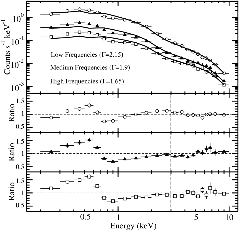
Figure 3: The LF, MF and HF Fourier energy spectra (open circles, filled triangles and open squares, respectively) plotted together with the “best-fitting” power-law models in the $>3$ keV band (solid lines; see text for details). The lower panels show the ratio of the Fourier spectra to the best fitting model.

In order to get additional insight into the broad band energy spectra of the different frequency components we produced count spectra for power law models with only Galactic absorption and slope increasing from $\Gamma=1.5$ to $\Gamma=2.5$ with a step of $\Delta\Gamma=0.05$. The power law normalizations were adjusted so that the total counts in the model and the LF, MF and HF energy spectra be equal (the appropriate auxiliary files for the creation of the model spectra were produced using the RMFGEN and ARFGEN tasks of SAS). The upper panel in Fig. 3 shows the LF, MF and HF energy spectra along with the model spectrum that fits each “best” at $E>3$ keV, i.e. gives the minimum sum of squared residuals (weighted by the data errors square) among the model spectra considered. The lower three panels in the same Figure show the ratio of the data to the best fitting model. Our model fitting results show that the spectral slope decreases from the LF to the HF band. We find that above 3 keV the LF, MF and HF spectra are well described by a power law model with $\Gamma=2.15,1.9$, and 1.65, respectively. When we fit the data/model ratios above 3 keV with a constant of value 1 we find $\chi^{2}=11.6,15.1,$ and 11.2/10 dof, respectively. We conclude that there is no strong evidence for the presence of an iron line in any of the three Fourier spectra. Furthermore, although the hard power law component is variable on all time scales (i.e. all three Fourier frequency bands), its slope does not remain constant. For example, there is a significant difference of $\Delta\Gamma=0.5$ in the hard band power law slopes of the LF and HF components. In other words, we find that the high frequency component has harder spectrum than that of the lower frequency one.

3.2 Model fits to the full band energy spectrum

At energies below $\sim 2$ keV, a simple power law model with Galactic absorption does not fit well the spectra of any of the three Fourier frequency bands. In all cases, the plot of the data/model ratio as a function of energy is qualitatively similar to the respective plot in the case of the power law model fit to the total energy spectrum (shown on the top of the lower panel in Fig. 2): we observe a strong, broad absorption feature at energies $\sim 0.7-2$ keV, and a broad “hump” at lower energies, whose amplitude appears to increase with increasing frequency. We modeled the soft X-ray band spectrum both for the entire data set and the three Fourier components as follows.

Since we have undersampled the energy resolution of the EPIC-PN data, it is possible to model the soft X-ray complex features considering simple, phenomenological components such as power laws and absorption edges (as opposed to constructing physical models of the absorber and the emitting source). To this end, following Turner et al. (2003), we first considered the entire energy spectrum being the sum of two power laws, one for each of the soft and hard bands, joining at an energy $E_{\rm break}=1$ keV and with $\Gamma_{\rm soft}>\Gamma_{\rm hard}$. Furthermore, in addition to Galactic neutral absorption, we also considered the possibility of intrinsic cold absorption as well. We produced count spectra keeping $\Gamma_{\rm hard}$ fixed to the value 2, and $\Gamma_{\rm soft}$ increasing from 2.05 to 3 in steps of $\Delta\Gamma=0.05$. In each step, we produced three different spectra with $N_{\rm H,intr}=10^{20},10^{21},$ and $10^{22}$ cm^-2. We found that the model spectra with $\Gamma_{\rm soft}\sim 2.4-2.6$ and $N_{\rm H,intr}=10^{20}$ cm^-2 agree “best” with the observed spectrum.

We then produced a new set of model spectra with $\Gamma_{\rm soft}=2.4-2.6$, and $N_{\rm H,intr}=10^{20}-10^{21}$ cm^-2 (using $\Delta\Gamma=0.05$ and $\Delta N_{\rm H,intr}=10^{20}$ cm^-2, respectively). Following Wilms et al. (2001), at each spectrum corresponding to a given pair of $(\Gamma_{\rm soft},N_{\rm H,intr})$ values we also added absorption edges at 0.74, 1 and 1.36 keV (these threshold energies correspond with the expected absorption edges of OVII, NeIX/MgX, and NeX). As for the optical depth, we used values of $\tau=0.5-1$ for the first edge, and $\tau=0-0.5$ in the other two cases, with a step of $\Delta\tau=0.1$. We then compared each $(\Gamma_{\rm soft},N_{\rm H,intr},\tau_{0.74keV},\tau_{1\rm keV},\tau_{1.36\rm keV})$ model with the observed spectrum in order to find the one with the minimum $\chi^{2}$.

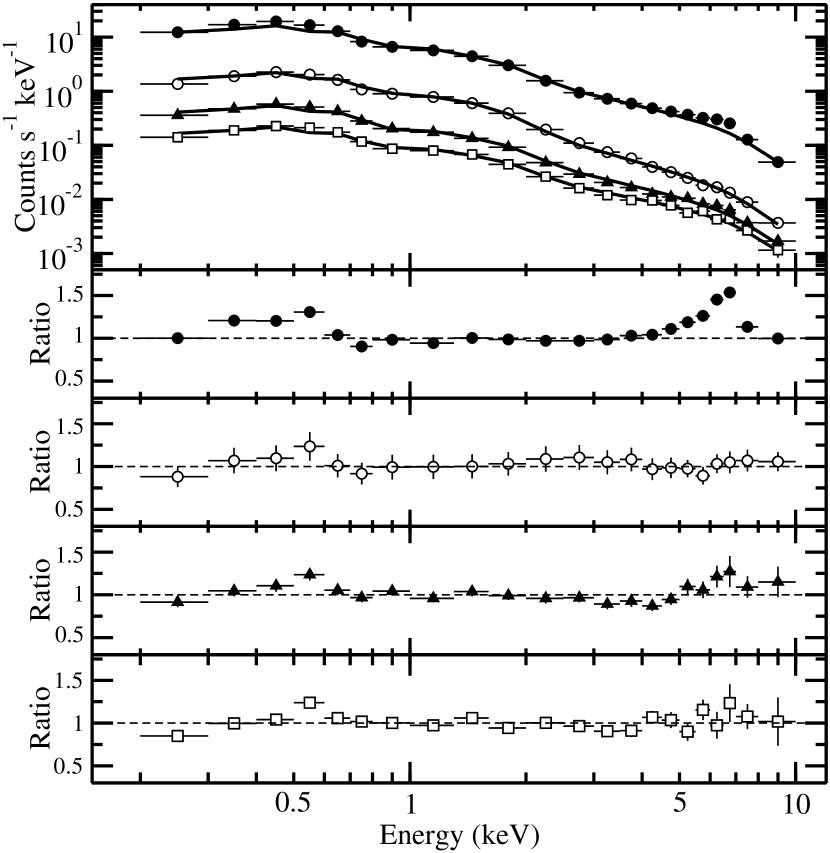
Figure 4: The total, LF, MF and HF Fourier energy spectra (filled circles, open circles, filled triangles and open squares, respectively) plotted together with the “best-fitting” model discussed in Section 2.2.2. The lower panels show the ratio of the spectra to the respective best fitting model.

The filled circles on the upper panel of Fig. 4 show the total energy spectrum of the source, together with our “best fitting model”: $\Gamma_{\rm soft}=2.5,N_{\rm H,intr}=3\times 10^{20}$ cm^-2, and $\tau_{0.74\rm keV}=0.7,\tau_{1\rm keV}=0,$ and $\tau_{1.36\rm keV}=0.2$. The data/model ratio is plotted on the second panel of the same Figure. The model describes rather well the overall shape of the spectrum, except in the vicinity of the Fe K$\alpha$ line and the $0.3-0.6$ energy band, where a strong ‘hump’ is evident. As discussed earlier, this feature has been attributed to relativistically broadened K$\alpha$ emission from oxygen (Branduardi-Raymont et al. 2001, Sako et al. 2003). Another possibility is that the gas responsible for the extra absorption within MCG -06-30-15 may not be cold but partially ionized. In this case, the depth of the neutral oxygen edge at $\sim 0.54$ will be smaller, reducing the discrepancy between model and observed spectra in this energy band (Turner et al. 2003).

Based on the results of the best fit procedure used to model the total spectrum, we examined whether a similar procedure could provide acceptable fits to the spectra of the individual Fourier components as well. The open squares in the upper panel of Fig. 4 correspond to the HF Fourier spectrum while the solid line shows the best fitting “broken power law with intrinsic absorption and two edges” model. The model parameter values are listed in Table 1. The bottom panel in the same Figure shows the data/model ratio. Apart from the point in the $0.5-0.55$ keV band, the model fits the spectrum quite well ($\chi^{2}=24.6/21$ dof). A similar model (without the presence of an edge at 1.36 keV) fits reasonably well the LF spectrum as well ($\chi^{2}=17.4/21$ dof when we omit the point at $\sim 0.5$ keV; the normalized residuals in this case are plotted in the third panel from top in Fig. 4, and the best fitting model parameters are listed in Table 1). In the case of the MF spectrum, the addition of an extra edge at 0.85 keV (the threshold energy of the O VIII edge) is necessary to provide a good fit ($\chi_{2}=26.7/21$ dof, if the $\sim 0.5$ point is again not taken into account; see second panel from bottom in Fig. 4 for the data/model ratio plot in this case, and Table 1 for the model fitting results).

In summary, the overall spectrum of the source is well described by two power law components (one for the low energy and one for the high energy sections of the spectrum), intrinsic absorption, as well as two absorption edges. These distinct power law components are present in the spectra of the individual Fourier components as well, indicating that they are variable. However, contrary to the hard band power law, $\Gamma_{\rm soft}\sim 2.5$, independent of the Fourier frequency, suggesting a different physical origin between these two components. Obviously, this result is somehow model dependent. Since the broken power law is a simple phenomenological model, there is no reason to exclude an alternative parametrization of the observed spectra, which may lead to different results, regarding the variability properties of the soft excess.

Finally, absorption features are evident in the spectra of all three Fourier components. The $\sim 0.7$ keV absorption edge appears to be equally strong (with $\tau\sim 0.7$) in all Fourier spectra. An edge at $\sim 1.36$ keV ($\tau\sim 0.2-0.3$) is evident in the MF and HF spectra, and a third edge (at $\sim 0.85$ keV; $\tau\sim 0.25$) is present in the MF spectrum only. The differences in the presence of edges in the three Fourier spectra could be due to the fact that the MF spectrum has the highest signal to noise ratio among them. For example, the addition of two edges at 0.85 and 1.36 keV (with $\tau=0.25$ and 0.2, respectively) in the LF best fitting model is acceptable at a confidence level of $\sim 10$%, while the addition of a 0.85 keV edge ($\tau=0.25$) in the HF best model fitting spectrum provides an acceptable fit at the $\sim 5$% level.

4 Discussion, Conclusions

We have applied the Fourier frequency resolved spectral analysis method to the XMM-Newton data of MCG -06-30-15. This work represents the first application of this method to the X-ray data of an AGN. Our main results are the following: a) The soft and hard bands of the spectrum of MCG -06-30-15 exhibit different RMS variability at different Fourier frequencies (time scales). b) Both the soft and hard band power law components are variable on all time scales. However, while the hard band power law becomes progressively steeper with decreasing Fourier frequency by $\Delta\Gamma\sim 0.25$ between each of the HF, MF and LF bands, no spectral slope variations are observed in the soft band power law component. c) An iron line, while present and clearly broad and asymmetric in the energy spectrum of the entire observation of this source, it is apparently absent in the energy spectra of the HF, MF and LF bands. d) A significant edge-like feature at $E\simeq 0.7-2$ keV is present in the spectra of all frequency bands.

Past studies based on “excess variance” analysis of $\sim 1$ day long light curves have shown that the variability amplitude in AGN is higher in the soft than the hard band (Nandra et al. 1997a, Leighly 1999). However the variance, being the integral of the power spectrum over frequency, say from $\nu_{\rm min}$ to $\nu_{\rm max}$, does not provide information on the variability amplitudes at the different time scales. This information, on the other hand, is provided by the Fourier resolved spectra obtained in our analysis. We thus find that the hard band variations are of larger amplitude than the soft band ones on time scales shorter than $\sim 3$ ksec, while the opposite effect is observed on time scales longer than 10 ksec. The distinctly different timing properties of these two bands, in conjunction with their very different spectra argue that they represent emission by different physical components, likely of different physical dimension.

However, even within the hard band itself, the spectral properties do depend on the Fourier frequency, as the spectra become softer with decreasing Fourier frequency. This can be attributed to the fact that the hard band fast varying components have spectra significantly harder than those of slower ones, or alternatively, that the higher energy variations are consistently shorter than those of lower energies. This result is not consistent with the suggestion of Vaughan & Fabian (2004) that the spectral variability of MCG -06-30-15 over the entire $0.2-10$ keV band can be explained by the presence of a constant component and a power law component which varies only in normalization.

On the other hand, this conclusion is in agreement with the power spectrum analysis of the XMM-Newton data of MCG -06-30-15 by Vaughan et al. (2003) who find that the power spectrum becomes flatter with increasing energy above the “break” frequency of $\sim 10^{-4}$ Hz. Similar behavior (power spectrum hardening at high frequencies with increasing energy) has been recently observed in other AGN (NGC 7469: Papadakis, Nandra & Kazanas, 2001; Mkn 766: Vaughan & Fabian, 2003; NGC 4051: McHardy et al. 2004, and 1H 0707-495, Ton S180 with the use of structure functions, Leighly 2004), as well as in the galactic black hole candidate Cyg X-1. This result by itself, ignoring the constraints imposed by the presence and variability properties of the soft band, could be interpreted as variability due to a Comptonizing corona of decreasing electron temperature with radius, along the general lines discussed in Kazanas, Hua & Titarchuk (1997).

The same interpretation, however, is not consistent with the variability of the soft component whose slope seems independent of the Fourier frequency. At this point, in the absence of lower energy data and based on the general shape of this component we are willing to speculate that it is due to emission by a (non-standard) accretion disk. As such we have in mind the ADIOS flows of Blandford & Begelman (1999). Assuming a viscosity parameter $\alpha\simeq 0.3$, a black hole mass $M\simeq 10^{6}$ M_⊙ and a disk size $R\simeq 10\;R_{S}$, we obtain a characteristic variability scale $t_{\rm var}\simeq(R/c)\alpha^{-1}(R/R_{S})^{3/2}\simeq 10^{4}$ s, in agreement with observations. The disk photons could then serve as the seeds needed to produce the harder power law component by hot electrons in a corona interior to and/or overlying part of this disk. In this respect, one should bear in mind that the lags between the soft (0.2-0.7 keV) and the hard (2-10 keV) bands (Vaughan et al., 2003) are in general agreement with such an interpretation and the observed tight correlation between the light curves of the soft and hard spectral components.

The results of our analysis indicate that the Fe K$\alpha$ line shows no significant variations on time scales shorter than $\sim 1-2$ days and are in agreement with the results of the previous studies (e.g. Vaughan & Fabian 2004, and references therein). The only grounds for concern in this conclusion is the MF energy spectrum. First of all, the residuals around $\sim 5-7$ keV in the “data/best model” ratio plot (Fig. 3 and 4) are suggestive of the presence of a line feature (albeit of small amplitude). Furthermore, if the MF spectrum were consistent with a just power law of index $\Gamma=1.9$, we would expect a decrease in the above ratio by $\sim 40$% in the $5-7$ keV band (the strength of the line above the $\Gamma=1.9$ power law in the total spectrum; see top plot in the bottom panel of Fig. 2), but we observe a smaller drop ($\sim 15$%), in the “MF/total spectrum” ratio (Fig. 2), a value that implies a possible difference in the true MF slope from the assumed value of $\Gamma=1.9$. We plan to investigate this issue further with the use of more data from recent Chandra, RXTE and ASCA observations of the source.

Our conclusions are similar to those of Revnivtsev et al. (1999) for Cyg X-1 in its low/hard state. They found the Equivalent Width (EW) of the iron line in the spectrum of the $\sim 1$ Hz and $\sim 10$ Hz Fourier components to be 80 and 50 eV, respectively. We find the $3\sigma$ upper limit in the EW of the line to be $\sim 60$ eV in the spectrum of the $\sim 10^{-5}-10^{-4}$ Hz components in MCG -06-30-15. The ratio of these frequency bands in the two sources is $\sim 10^{5}$, roughly comparable to the ratio of the black hole mass in the two systems, if we assume a $10$ M_⊙ and $\sim 10^{6}$M_⊙ mass for Cyg X-1 and MCG -06-30-15 (McHardy et al. 2005), respectively. As noted by Revnivtsev et al. (1999), the most straightforward interpretation of the absence of a line in the frequency resolved spectra of frequency higher than $\nu_{k}$ is that the X-ray reprocessing matter is located at a distance $R_{\rm rep}\mathrel{\raise 2.15277pt\hbox{$>$}\mkern-14.0mu\lower 2.58334pt\hbox{$\sim$}}c\cdot[\nu_{k}/2\pi]^{-1}$. For $\nu_{k}\simeq 10^{-5}$ Hz this is $R_{\rm rep}\sim c\cdot 15000~{}{\rm s}\simeq 4.5\times 10^{14}$ cm, or $1500R_{S}$ for a $10^{6}$ M_⊙ black hole mass. If this is indeed the case, the line flux light curve should be much smoother than that of the continuum, and its variations should be of amplitude smaller than that of the continuum, a fact in agreement with observations (e.g. Vaughan & Fabian 2004). However, such large distances are hard to reconcile with the observed line width that requires line emission size $R_{\rm rep}\mathrel{\raise 1.29167pt\hbox{$<$}\mkern-14.0mu\lower 3.44444pt\hbox{$\sim$}}10R_{S}$. Recently, Miniutti et al. (2003) suggested that this lack of variability could be explained by a combination of light bending effects and vertical motions of the X-ray source above the accretion disk. Alternatively, the large width of the line maybe due to its downscattering in an expanding wind, as suggested recently by Titarchuk, Kazanas & Becker (2003). Inoue & Matsumoto (2003) also argue that the large width of the line is an artifact caused by the fact that the continuum suffers from absorption by various layers of warm absorbing material with variable column density and/or covering factor on time scales $\sim 10^{5}$ s. In this case, we should observe absorption features in the $5-8$ keV band of the Fourier spectra, but none are clearly evident in the residual plots (Fig. 3 and 4).

Of particular interest is the feature at $\simeq 0.7$ keV, which is easily discernible in the energy spectra of all 3 frequency bands. It has been attributed to a combination of O VII edge and FeI absorption (Turner et al.2003). In this case one can set a limit on the distance of the absorber, assuming that the later remains unaffected by the changes in the continuum flux; this assumption is justified by the absence of a strong dependence of this feature’s depth on the Fourier frequency. This sets a limit to the value of the photoionization parameter of the absorbing medium to values $\xi=L/n\,R^{2}\mathrel{\raise 1.29167pt\hbox{$<$}\mkern-14.0mu\lower 3.44444pt\hbox{$\sim$}}30$ erg cm/s. On the other hand, the depth of the feature sets also a limit on the column density of the absorbing gas $N_{H}=n\,R\simeq 10^{22}$ cm^-2, values consistent with the detailed models of Turner et al. (2003); this results, then, in $R\simeq L/\xi\,N_{H}\simeq 10~{}{\rm pc}~{}(L_{43.5}/\xi_{1.5}N_{H_{22}})$, where the subscripts denote the base 10 exponent of the value of the corresponding parameter in cgs units.

As we have already mentioned, the same feature along with the spectral “hump” in the residual plots of Fig. 4 around 0.5-0.55 keV has been interpreted as a relativistically broadened O K$\alpha$ line. The presence of this feature in the spectra of all Fourier components (and in particular those of highest Fourier frequency) is, taken at face value, consistent with such an interpretation. Interestingly, an absorption feature by matter with properties obtained in the previous paragraph would also conform with the same phenomenology. On the other hand, the broad Fe K$\alpha$ line which is modeled as emission by plasma in the same physical location as that responsible for an O K$\alpha$ line, has very different timing properties, as it is absent from any of the Fourier resolved spectra. This difference in the timing properties of these two components that have presumably their origin in the kinematics of the same plasma makes the presence of a soft X-ray line suspect. In addition, when one considers the effects of the highly variable hard X-ray component on the ionization structure of the line emitting plasma that would highly ionize the accretion disk plasma (Nayakshin, Kazanas & Kallman 2000; Nayakshin & Kazanas 2001), the interpretation of this feature as a relativistically broadened O K$\alpha$ line becomes doubtful.

In conclusion, the Fourier resolved spectroscopy technique discussed in the present work is a powerful instrument in analyzing the spectro-temporal properties of AGN and accreting compact objects in general. By attributing specific spectral properties/features to specific Fourier frequencies/time scales it allows one to further dissect the structure of these sources. It is hoped that the additional information provided by this technique will allow for a deeper understanding of this structure and the associated physics. Our work is but a first step in this direction. At this point it is not clear whether the properties implied by our analysis represent general AGN trends or idiosyncrasies of MCG -06-30-15. We hope that analysis of additional objects along the same lines will help decide this question.

Table 1: Best fitting values of the “broken power law plus absorption edges” model parameters, for the LF, MF, and HF Fourier spectra (FS). The uncertainties quoted are at the 90 per cent level for one interesting parameter. They are multiple of the respective parameter step size used in the construction of the various models, and correspond to the values which increase $\chi^{2}$ (when omitting the point at 0.55 keV) by $\Delta\chi^{2}\mathrel{\raise 2.15277pt\hbox{$>$}\mkern-14.0mu\lower 2.58334pt\hbox{$\sim$}}2.71$, keeping the other parameters fixed to their best fitting values.

FS	NH	$\Gamma_{\rm hard}$	$\Gamma_{\rm soft}$	$\tau_{0.74\rm keV}$	$\tau_{0.85\rm keV}$	$\tau_{1.36\rm keV}$
	$\times 10^{20}$ cm-2
LF	$3\pm 1$	$2.25\pm 0.05$	$2.4\pm 0.15$	$0.7^{+0.4}_{-0.25}$	$-$	$-$
MF	$3\pm 1$	$2^{+0.10}_{-0.05}$	$2.45\pm 0.1$	$0.7^{+0.15}_{-0.1}$	$0.25\pm 0.15$	$0.3^{+0.15}_{-0.1}$
HF	$3\pm 1$	$1.7\pm 0.05$	$2.5^{+0.05}_{-0.15}$	$0.8\pm 0.15$	$-$	$0.2^{+0.15}_{-0.1}$

References

- (1) Blandford, R. D. & Begelman, M. C. 1999, MNRAS, 303, L1
- (2) Branduardi-Raymont, G, Sako, M., Kahn, S. M., Brinkman, A. C., Kaastra, J. S., & Page, M. J. 2001, A&A, 365, 140
- (3) Elvis, M., Wilkes, B. J., & Lockman, F. J. 1989, AJ, 97, 777
- (4) Fabian, A. C., Rees, M. J., Stella, L., & White, N. E. 1989, MNRAS, 277, 11
- (5) Fabian, A. C., et al. 2002, MNRAS, 335, 1
- (6) Inoue, H., & Matsumoto, C. 2003, PASJ, 55, 625
- (7) Kazanas, D., Hua, X.-M., & Titarchuk, L. 1997, ApJ, 480, 735
- (8) Lee, J. C., Iwasawa, K., Houck, J. C., Fabian, A. C., Marshall, H. L., & Canizares, C. R. 2002, ApJ, 570, L47
- (9) Leighly, K. M. 1999, ApJS, 125, 297
- (10) Leighly, K. M. 2004, Progress of Theoretical Physics Supplement, 155, 223
- (11) McHardy, I. M., Papadakis, I. E., Uttley, P., Page, M. J., & Mason, K. O. 2004, MNRAS, 348, 783
- (12) McHardy, I.M., Gunn F.K., Uttley, P., & Goad, M. R. 2005, MNRAS, in press (astro-ph/0503100)
- (13) Miniutti, G., Fabian, A.C., Goyder, R., & Lasenby, A.N. 2003, 344, 22
- (14) Nandra, K., George, I. M., Mushotzky, R. F., Turner, T. J., & Yaqoob, T. 1997a, ApJ, 476, 70
- (15) Nandra, K., George, I. M., Mushotzky, R. F., Turner, T. J., & Yaqoob, T. 1997b, ApJ, 477, 602
- (16) Nayakshin, S., Kazanas, D., & Kallman, T. R. 2000, ApJ, 537, 833
- (17) Nayakshin, S., & Kazanas, D. 2001, ApJ, L141
- (18) Papadakis, I. E., Nandra, K., & Kazanas, D. 2001, ApJ, 554, L133
- (19) Revnivtsev, M., Gilfanov, M., & Churazov, E. 1999, A&A, 347, 23
- (20) Revnivtsev, M., Gilfanov, M., & Churazov, E. 2000, MNRAS, 316, 923
- (21) Revnivtsev, M., Gilfanov, M., & Churazov, E. 2001, A&A, 380, 520
- (22) Reynolds, C. S., Young, A.J., Begelman, M.C., & Fabian, A.C. 1999, ApJ, 514, 164
- (23) Sako, M., et al. 2003 ApJ, 596, 114
- (24) Stella, L. 1990, Nature, 344, 747
- (25) Tanaka, Y., et al. 1995, Nature, 375, 659
- (26) Titarchuk, L. G., Kazanas, D. & Becker, P., 2003, ApJ, 598, 411.
- (27) Turner, A. K., Fabian, A. C., Vaughan, S., & Lee, J. C. 2003, MNRAS, 346, 833
- (28) Uttley, P., McHardy I.M., & Papadakis, I.E. 2002, MNRAS, 332, 231
- (29) Vaughan, S., Fabian, A. C. & Nandra, K. 2003, MNRAS, 339, 1237
- (30) Vaughan, S., & Fabian, A. C. 2003, MNRAS, 341, 496
- (31) Vaughan, S., & Fabian, A. C. 2004, MNRAS, 348, 1415
- (32) Wilms, J., Reynolds, C. S., Begelman, M. C., Reeves, J., Molendi, S., Staubert, R., & Kendziorra, E. 2001, MNRAS, 328, 27L
- (33)