The Cornell High-order Adaptive Optics Survey for Brown Dwarfs in Stellar Systems–I: Observations, Data Reduction, and Detection Analyses

J. C. Carson¹¹affiliation: present address: Jet Propulsion Laboratory, Earth & Space Sciences, 4800 Oak Grove Dr., MS 183-900, Pasadena, CA 91109 ²²affiliation: Postdoctoral Scholar, California Institute of Technology. , S. S. Eikenberry³³affiliation: present address: Department of Astronomy, University of Florida, 211 Bryant Space Science Center, Gainesville, FL 32611 , B. R. Brandl⁴⁴affiliation: present address: Leiden Observatory, PO Box 9513, 2300 RA Leiden, The Netherlands , J. C. Wilson⁵⁵affiliation: present address: Department of Astronomy, University of Virginia, 255 Astronomy Building, PO Box 3818, Charlottesville, VA 22903 , and T. L. Hayward⁶⁶affiliation: present address: Gemini Observatory, Southern Operations Center, Casilla 603 La Serena Chile Department of Astronomy, Cornell University, Ithaca, NY 14853

Abstract

In this first of a two-paper sequence, we report techniques and results of the Cornell High-order Adaptive Optics Survey for brown dwarf companions (CHAOS). At the time of this writing, this study represents the most sensitive published population survey of brown dwarf companions to main sequence stars, for separation akin to our own outer solar system. The survey, conducted using the Palomar 200-inch Hale Telescope, consists of K_s coronagraphic observations of 80 main sequence stars out to 22 parsecs. At 1 $\arcsec$ separations from a typical target system, the survey achieves median sensitivities 10 magnitudes fainter than the parent star. In terms of companion mass, the survey achieves typical sensitivities of 25 M_Jup (1 Gyr), 50 M_Jup (solar age), and 60 M_Jup (10 Gyr), using evolutionary models of Baraffe et al. (2003). Using common proper motion to distinguish companions from field stars, we find that no systems show positive evidence of a substellar companion (searchable separation $\sim$ 1-15 $\arcsec$ [projected separation $\sim$ 10-155 AU at the median target distance]). In the second paper of the series we shall present our Monte Carlo population simulations.

stars: low-mass, brown dwarfs — surveys — techniques: high angular resolution — instrumentation: adaptive optics — instrumentation: high angular resolution — methods: data analysis

^†^†slugcomment: Accepted by Astronomical Journal. Expected publication date: September 2005.

1 Introduction

The discovery of the brown dwarf Gl 229B (Nakajima et al. 1995) heralded a stream of direct detections of sub-stellar objects. Field surveys such as the Two Micron All-Sky Survey (2MASS; Skrutskie et al. 1997), the Deep Near Infrared Survey (DENIS; Epchtein et al. 1997), and the Sloan Digital Sky Survey (SDSS; Gunn and Weinberg 1995) helped raise the number of brown dwarf identifications today to close to a thousand. But despite these advances, the search for brown dwarf companions at intermediate and narrow separations (say less than a few arcseconds) to main sequence stars remains difficult. Despite a strong community effort in high-contrast imaging observations, less than a half-dozen companions have been confirmed as $<$ 100 AU (projected separation) substellar companions to main sequence stars.

To date, the most comprehensive probe of ultra-narrow separation ( $\lesssim$ 10 AU) brown dwarf companions comes from radial velocity surveys such as Marcy & Butler (2000) : McCarthy & Zuckerman (2004), for instance, report that over 1500 F, G, K, and M stars have been observed, via this method, with sensitivities strong enough to detect brown dwarf companions between 0 and 5 AU. Using observations like these, Marcy & Butler (2000) conclude that the $\leq$ 3 AU brown dwarf companion fraction to F-M stars is less than 0.5 $\%$ . High angular resolution imaging surveys such as CHAOS, a deep adaptive optics (AO) coronagraphic search and proper motion follow-up of faint companions, are required to test if this low companion fraction extends out to intermediate distances, akin to our own outer solar sytem. Knowledge of these intermediate separation companions will help bridge the gap between radial velocity companion surveys and wide-separation companion data such as 2MASS. The CHAOS survey is not the first study to examine this search space. Recently published intermediate separation coronagraphic surveys include Liu et al. (2002), Luhman & Jayawardhana (2002), McCarthy & Zuckerman (2004), Metchev & Hillenbrand (2004), and Potter et al. (2002). Unlike these other surveys however, the CHAOS paper here represents, at the time of this writing, the only published adaptive optics survey that reports complete results for all surveyed targets, including null result observations. Reporting comprehensive results on all surveyed targets, this CHAOS paper invites a rich opportunity for statistical inquiry into brown dwarf and stellar formation theory.

In the sections below we present techniques and results for the recently completed CHAOS survey. Section 2 presents our target sample. Section 3 describes our observing techniques. In Section 4 we present the data analysis techniques we developed for this survey. In Section 5 we summarize our survey sensitivities. Section 6 describes our results. We present our conclusions in Section 7.

2 Target Sample

We began our candidate selection process with a careful review of the Third Catalogue of Nearby Stars (Gliese & Jahreiss 1995). Beginning with northern stars, we prioritized targets by their closeness to our solar system. Next we discarded all stars that exist in known resolvable multiple systems, as this scenario would prevent us from effectively hiding the entire parent system behind the 0. $\arcsec$ 9 coronagraphic mask. We double-checked for the presence of stellar companions using Hipparcos data (Perryman et al. 1997) as well as on-telescope preliminary imaging. The one known (Perryman et al. 1997) resolvable binary that we kept was Gliese 572; For this target, the secondary star’s narrow separation ( $\sim$ 0. $\arcsec$ 4) allowed us to hide both stars behind the 0. $\arcsec$ 9 coronagraphic spot, to an acceptable level. We did not delete spectroscopic binaries from the target list as these unresolved targets allowed for effective coronagraphic masking; Gliese 848, 92, 567, 678, and 688 of our final target list are known spectroscopic binaries, as published in Pourbaix et al. (2004). As the next step, we removed all stars with a V magnitude fainter than $\sim$ 12 mags. Our previous experience using Palomar Adaptive Optics (PALAO) in 2000 indicated that stars fainter than this limit were unable to serve as effective natural guide stars. Next we searched the USNO-A2.0 Catalogue (Monet et al. 1998) for a corresponding point spread function (PSF) calibration star for each targeted star. For choosing a PSF calibration star, we required the following restrictions: 1) A separation less than a couple degrees from the target star; 2) A difference in V magnitude, relative to the target star, $\lesssim$ 1 mag; 3) An absence of any known resolvable companions. These restrictions ensured that the calibration star would deliver a measured PSF similar to the target star’s PSF. Any target star that did not have a corresponding calibration star meeting this criterion was removed from the sample. We expanded the search region further and further south from the original northern positions until the list included a total of 80 stars extending as far south as -10 degrees inclination. This final target sample included 3 A stars, 8 F stars, 13 G stars, 29 K stars, 25 M stars, and 2 stars with ambiguous spectral types. All stars possessed well-characterized proper motion values as defined by Hipparcos (Perryman et al. 1997). As nearby stars, they typically possessed high proper motion (median target proper motion $\sim$ 600 mas/yr) thus facilitating an efficient common proper motion follow-up strategy for candidate companions. A complete list of the target set is given in Table 1.

In the second paper of this series, we will present a thorough discussion of how selection biases in our sample may affect derived brown dwarf populations. For the time being, however, we do note that certain formation models, such as ones that support the creation of brown dwarfs within multiple systems (Clarke, Reipurth, & Delgado-Donate 2004 for example), imply that observed population levels, as derived from our mostly single-star sample, may differ significantly from statistics that include multiple systems.

3 Observations

3.1 Coronagraphic Search Observations

To conduct our survey, we used the Palomar Adaptive Optics system (PALAO; Troy et al. 2000) and accompanying PHARO science camera (Hayward et al. 2001) installed on the Palomar 200-inch Hale Telescope. PALAO provided us with the high resolution (FWHM typically $\sim$ 0 $\arcsec$ .14 in K-short) necessary for resolving close companions. The accompanying PHARO science camera (wavelength sensitivity 1-2.5 $\micron$ and platescale 40 mas per pixel) provided us with a coronagraphic imaging capability along with a field of view ( $\sim$ 30 $\arcsec$ ) substantially larger than any competitively sized telescope’s adaptive optics system, at the time of the survey’s commencement.

Our general observing strategy was to align the coronagraphic mask on a target star and take a series of short exposures as to not saturate many pixels in the detector. (Occasionally we saturated at the edges of the coronagraphic mask where high noise levels already prevented any meaningful companion search.) We planned our exposure time and number of exposures to allow for a maximum 8 minutes of execution time (including overheads). This helped ensure that sky conditions did not significantly change between the target exposures and following PSF calibration star exposures. When target star exposures were complete, we spent a similar amount of time taking coronagraphic images of the PSF calibration star. Immediately flanking this target pair, we took dithered images of a nearby empty sky region, using the same set-up as the target and reference star series. We repeated this process (sky, target, reference star, sky) as many times as necessary to reach our desired signal to noise. Once we completed these image sets, we inserted a neutral density filter in the optical path and conducted dithered non-coronagraph exposures of the target star. These images allowed us to characterize and record instrument and site observing conditions. Table 1 describes relevant observing information for the individual targets.

3.2 Common Proper Motion Observations

For candidate companions detected in the previous procedures, we checked for a physical companionship by using common proper motion observations. The nearby stars we observed tend to have high proper motions (on the order of a few hundred mas yr^-1). The vast majority of false candidate companions are background stars that tend to have very small proper motions compared to the parent star. Therefore, after recording our initial measurement, we waited for a timespan long enough for the parent star to move a detectable distance, typically $\gtrsim$ 3 sigma separation from the original position. We then repeated our observing set so that we could check to see if the candidate maintained the same position with respect to the parent star. Target stars re-observed to check for common proper motion include Gliese 740, 75, 172, 124, 69, 892, 752, 673, 41, 349, 412, 451, 390, 678, 768, 809, 49, and 688. Due to instrument scheduling constraints, Gliese 49, 41, 390, and 678 were all re-observed using the Palomar 200-inch Wide-field Infrared Camera (WIRC; Wilson et al. 2003) rather than PALAO and the accompanying PHARO science camera. Since the WIRC camera possesses no coronagraphic mode, the observations were instead conducted using standard dithered exposure sequences. WIRC, with its non-AO-corrected point spread function and lack of a coronagraphic mask, made a poorer probe of astrometry than the PHARO camera. However, the systems observed with WIRC all possessed large expected proper motions ( $>$ 400 mas [1 WIRC pixel $\sim$ 250 mas]) and large separations ( $>$ 10 arcseconds) from the parent system, making them acceptable WIRC observing targets.

4 Data Analysis

4.1 Reducing Images

We began our data reduction by median-combining each of the dithered sky sets. We then took each coronagraphed star image and subtracted the median-combined sky taken closest in time to the star image. (The typical separation in time between target and sky image was $\sim$ 5.5 minutes.) We divided each of the sky-subtracted star images by a flatfield frame that we created, using standard procedures, from twilight calibration images taken that same night. Next we median-combined each sequence of coronagraphed star frames. For this median-combination, we used the images’ residual parent star flux (that leaked from around the coronagraph) to realign any frames that may have shifted due to instrument flexure. Next we applied a bad pixel algorithm to remove suspicious pixels (defined as any pixel deviating from the surrounding 8 pixels by $\geq$ 5-sigma) and replace them with the median of their neighbors.

After completing this procedure for both target star and calibration star image sets, we scaled the calibration star PSF so that two 50-90 pixel annuli, one centered on the target star, the other centered on the scaled PSF, exhibited identical median values. Next we multiplied the scaled PSF by test values ranging from 0.20 to 1.76 at 0.04 intervals. For each test value we also tried shifting the scaled PSF -7 to +7 pixels, at integar steps, in each of the x and y directions. From these test combinations we selected the adjusted PSF that most closely resembled the target star, according to a least-squared fit of flux values 50 to 90 pixels from the star center. We next subtracted our adjusted PSF from the target star to arrive at a final image for the set. In the cases where we had multiple target star/calibration star observing set pairs, we co-added the final images, using the residual parent star PSF to correct any misalignments.

As our final data reduction procedure, we applied a Fourier filter to help remove non-point-like features such as unwanted internal instrument reflection and residual parent star flux. The Fourier filter application entailed our multiplying each pixel in a Fourier transformed version of the final image (where the lowest frequencies resided at the center of the array and largest frequencies resided toward the edges) by e ${}^{\frac{r-23}{34}}$ . r here is the separation, in units of pixels, between a given pixel and the center of the Fourier transformed array. We then applied an inverse Fourier transform to the array to produce the final filtered image. We chose the two aforementioned numerical parameters (23 and 34) of our exponential function after first running test trials on a crowded field image using a generic exponential function e ${}^{\frac{r-m}{\sigma}}$ . For these trial functions we set m to test values ranging from 5 to 49, at integar values; We set $\sigma$ to test values ranging from 1 to 39, again at integar intervals. Testing all combinations, including an equivalent gaussian version as well, we found that e ${}^{\frac{r-23}{34}}$ produced the greatest signal-to-noise improvements. For sampled field stars in our tests, signal-to-noise levels improved by about 25% between non-filtered and filtered images. Along with this signal-to-noise improvement, the typical PSF FWHM decreased by about 10% as a result of the Fourier filter application.

4.2 Identifying Brown Dwarf Companions

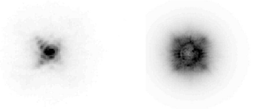
Our first step in identifying brown dwarf companions was to individually inspect each final psf-subtracted and non-psf-subtracted image for any potential companions. By choosing to examine both subtracted and non-subtracted final images, we effectively recognize that the PSF-subtraction improves our ability to identify candidates close to the parent star, but, due to the introduced increased sky noise, makes it more difficult to identify candidates at larger separations from the parent star. For our identifications, the characteristic Palomar adaptive optics “waffle pattern” (see Figure 1) helped distinguish real objects from false ones. Practically, we found that this individual inspection was the most effective method of identifying candidate companions. However, for the purpose of determining quantifiable detection sensitivities, we chose to use an automated detection system as well.

Our automated algorithm operated by centering on every other pixel in the image array and creating there a 0. $\arcsec$ 16 diameter flux aperture and 1. $\arcsec$ 2-1. $\arcsec$ 6 diameter sky annulus. After subtracting any residual sky background, the algorithm approximated a signal-to-noise level by dividing the measured aperture flux by the combined aperture flux Poisson noise and background noise; It approximated background noise from the standard deviation of the sky annulus pixels. In the end it outputted a final array with a signal-to-noise value for each sampled pixel. For each signal-to-noise map, it also generated a map of measured background noise at each position (as estimated from the sky annuli). This outputted noise map essentially reflected the ability of the algorithm to detect (at a given thresh-hold signal-to-noise level) different brightness objects according to position on the array.

After generating maps for a given image, the program selected the signal-to-noise map pixel with the highest value, using a minimum value of five. It recorded the pixel position and then moved on to record the next highest signal to noise value greater than five. After each detection, it voided a 0. $\arcsec$ 4 radius around the detected candidate object. This procedure continued until there were no more positions with signal to noise values greater or equal to five. (Of course, for many images, no positions possessed signal to noise levels greater than five.) After the algorithm identified the candidate sources, we re-examined the final images to ensure that the algorithm had indeed detected a true source as opposed to a systematic effect. Again, we searched for the Palomar adaptive optics signature “waffle pattern” to ensure a true physical source. We also made comparisons to images taken at other sources to ensure that the feature was indeed unique to the target image.

We acknowledge that the use of our automated detection routine has some drawbacks. Notably, there are several instances where the algorithm over-estimates the noise level in the non-psf-subtracted and psf-subtracted images. For instance, when examining the non-psf-subtracted images at regions near the parent star, the algorithm can mistake what may be a well-ordered parent star PSF slope for a random fluctuation in background noise. In this instance, fortunately, the subsequent examination of the corresponding psf-subtracted image should ensure that the initial over-estimation in noise does not affect final results. However, such a correction will not occur when the algorithm is hunting around field stars; If a field star happens to fall in the sky annulus, the algorithm will determine that region to have excessively high background noise. Thus, only the brightest candidate objects would be detected near these field star positions. In Section 5 we discuss how we may generate limiting magnitudes and brown dwarf mass limits from these algorithm-generated noise maps.

In cases where we positively identified a potential brown dwarf companion to a parent star, we next estimated its apparent K_s magnitude, using the non-coronagraphed calibration images of the parent star and published 2MASS K-magnitudes (Skrutskie et al. 1997). Resulting magnitudes are displayed in Table 2. Once we established an apparent K_s magnitude, we derived a corresponding absolute K_s magnitude, assuming the candidate had a distance equal to the parent system. Thanks to observational surveys such as Hipparcos (Perryman et al. 1997), all of our parent stars had well-defined parallaxes and therefore distances. With an approximate absolute K_s magnitude in hand, we combined published brown dwarf observational data (Leggett et al. 2000, Leggett et al. 2002, Burgasser et al. 1999, Burgasser et al. 2000, Burgasser et al. 2002, Burgasser, McElwain, & Kirkpatrick 2003, Geballe et al. 2002, Zapatero et al. 2002, Cuby et al. 1999, Tsvetanov et al. 2000, Strauss et al. 1999, and Nakajima et al. 1995) with theoretical data from Burrows et al. (2001) to extrapolate constraints on the object’s mass. An object whose potential mass fell within acceptable brown dwarf restrictions was designated for common proper motion follow-up observations.

For our follow-up observations, we used Hipparcos published common proper motion values (Hipparcos catalogue; Perryman et al. 1997) to determine the expected movement of the parent system. Since background and field stars are unlikely to possess proper motions identical to the parent system’s, we used common proper motion as a strong support for a physical companionship. To determine the candidate companion’s relative position in different epoch images, we fit a gaussian profile to the candidate companion flux position. For the parent star, we determined position from an extrapolated gaussian profile created from the flux leaking from behind the coronagraphic mask. We could typically constrain the parent star position to within a pixel or two and the candidate position to a fraction of a pixel, depending on the signal-to-noise levels. Measuring the candidate companion’s relative position over the two epochs, we were able to distinguish physical companionships from chance alignments. We record positions in Table 2.

5 Survey Sensitivities

5.1 Determining Limiting Magnitudes

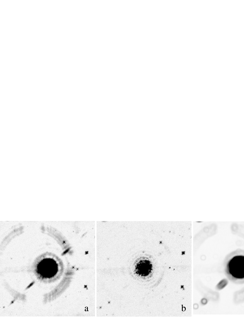
To quantify detection sensitivities from the algorithm-generated noise maps described in Section 4.2, we looked to determine the faintest detectable magnitude as a function of angular separation from each parent star. We began by sampling each of the final psf-subtracted and non-subtracted noise maps and selecting, for each pixel, the smaller of the two noise values. The resulting composite noise map array therefore reflected the best sensitivities from each of the two final images. Figure 2 displays a sample image sequence, where a psf-subtracted and non-subtracted image are combined to create a composite noise map.

Once we had generated our composite noise maps, we declared an array of sample apparent K_s-magnitudes extending from 8 to 23 mags at intervals of 0.3 mags. This selection included all potential brown dwarf magnitudes that we were likely to encounter. We do note that some of the lowest luminosity brown dwarfs may have magnitudes dimmer than our 23-magnitude limit. However, since 23 magnitudes was effectively beyond even our most optimistic sensitivity estimates, we did not need to consider anything fainter than that. We next transformed the apparent magnitudes to instrument counts using the parent star calibration data described in Section 3.1.

Returning to the composite noise map, we determined the median values in a series of concentric 0 $\arcsec$ .20-thick rings centered on the noise map center. The median values therefore represented typical noise as a function of distance from the central star. For each noise value, we then determined the minimum apparent K_s-magnitude where signal exceeded the combined Poisson noise and ring noise by a factor greater or equal to 5. In Figure 3 we plot resulting measurements for median survey sensitivities (middle curve), the best 10% of observations (lower curve), and the worst 10% of observations (top curve). Refer to Table 3 for a summary of minimum detectable magnitudes for each of the individual targets.

Another commonly used statistic for describing sensitivities for high-contrast companion surveys is the limiting differential magnitude as a function of angular separation from the parent star. In other words, how many times dimmer may a companion object be before we lose it in the parent star noise? Figure 4 plots differential magnitudes for median survey sensitivities as well as the best and worst 10% of observations.

5.2 Mass Sensitivities

Determining sensitivities according to companion mass is complicated by the fact that brown dwarfs of a given mass dim over time. Nonetheless, to get a general idea of detectable masses, we may assume different test ages and then use models by Burrows et al. (2001) or Baraffe et al. (2003) to transform our minimum detectable brightnesses into brown dwarf masses. Figure 5 shows a comparison of median sensitivities assuming 1 Gyr, solar age, and 10 Gyr target ages.

6 Results

After conducting all of our data analysis, we concluded that zero systems showed positive evidence of a brown dwarf companion. For Gliese 412 follow-up common proper motion observations, the available observing time was too short for us to positively confirm or reject common proper motion. 2MASS data tells us that, in the Gliese 412 neighborhood, the odds of our finding a field star in the PHARO field of view are about 1%. If it is a true companion, its magnitude would place it somewhere around an L9 dwarf classification. In a survey of 80 target stars, a 1% chance alignment is not particularly unusual, making a field star classification a reasonable potentiality. In the end though, these speculations cannot confirm or reject the presence of a true brown dwarf companion. At this point, we classify it as a non-brown dwarf detection until a time when we may confirm its substellar companion nature. Table 2 presents our discovered field stars meeting the automated detection routine’s sensitivity criteria.

7 Discussion

The observational data we have presented here clearly supports speculations of a “brown dwarf desert” at orbital separations comparable to our own outer solar system. However, we emphasize that we cannot definitively assert that a brown dwarf desert exists before applying rigorous Monte Carlo simulations that take into account any observational biases. For example, if the brown dwarf companion population were to have unusually high eccentricities, then the $\sim$ 100 AU projected separations that we believe we are investigating could in fact be representative of semi-major axes closer to 10 AU. In that case, the 100 AU (true semi-major axis) brown dwarf companion population could in fact be quite high since the members would spend the majority of their orbit outside of our field of view. To address this issue, we conducted full-scale Monte Carlo simulations that account for the effects of differing orbital parameters. In our upcoming paper (part II of this series) we discuss such population simulations at length. One important early result though of such simulations is that approximate analytical solutions presented in McCarthy & Zuckerman (2004) and Gizis et al. (2001), which assume zero inclination and zero eccentricity, suffer from sytematic observational biases that cause them to dramatically understate their uncertainties. Thus, we caution the reader against firmly asserting a brown dwarf companion desert before reading our entire upcoming analysis.

We thank Jean Mueller, Rick Burruss, Karl Dunscombe, and the Palomar Mountain crew for their support. We also thank Sarah Higdon and James Higdon for conducting observations for us. We thank our anonymous referee for their careful review and helpful suggestions. J. C. C. and S. S. E. were supported in part by NSF CAREER award AST-0328522. Facilities: Palomar Observatory(PALAO/PHARO,WIRC).

References

Baraffe et al. (2003) Baraffe, I., Chabrier, G., Barman, T. S., Allard, F., & Hauschildt, P. H. 2003, A&A, 402, 701
Burgasser et al. (1999) Burgasser, A. J., et al. 1999, ApJ, 522, 65
Burgasser et al. (2000) Burgasser, A. J., et al. 2000, AJ, 120, 1100
Burgasser, et al. (2002) Burgasser, A. J. et al., 2002, ApJ, 564, 421
Burgasser et al. (2003) Burgasser, A. J., McElwain, M. W., & Kirkpatrick, D. J., 2003, AJ, 126, 24 87
Burrows et al. (2001) Burrows, A., Hubbard, W. B., Lunine, J. I., & Liebert, J. 2001, Reviews of Modern Physics, 73, 719
Cuby et al. (1999) Cuby, J. G., Saracco, P., Moorwood, A. F. M., D’Odorico, S., Lidman, C., Comerón, F., & Spyromilio, J. 1999, A&A, 349, L41
Clarke et al. (2004) Clarke, C., Reipurth, B., & Delgado-Donate, E. 2004, RevMexAA, 21, 184
Epchtein (1997) Epchtein, N., 1997, in The Impact of Large-Scale Near-IR Sky Surveys,
ed. F. Garzon (Dordrecht: Kluwer), 15
Geballe et al. (2002) Geballe et al. 2002, ApJ, 564, 466
Gizis et al. (2001) Gizis, J. E., Kirkpatrick, J. D., Burgasser, A., Reid, I. N., Monet, D. G., Liebert, J., & Wilson, J. C. 2001, ApJ, 551, 163
Gliese & Jahreiss (1995) Gliese, W. & Jahreiss, H. 1995, VizieR On-line Data Catalog, 5070
Gunn & Weinberg (1995) Gunn, J. & Weinberg, D. 1995, WFSD Conf, 3
Hayward et al. (2001) Hayward, T. L., Brandl, B., Pirger, B., Blacken, C., Gull, G. E., Schoenwald, J, & Houck, J. 2001, PASP, 113, 105
Leggett et al. (2000) Leggett, S. K. et al. 2000, ApJ, 536, 35
Leggett, et al. (2002) Leggett, S. K. et al., 2002, ApJ, 564, L452
Liu et al. (2002) Liu, M. C., Fischer, D. A., Graham, J. R., Lloyd, J. P., & Butler, R. P. 2002, ApJ, 571, 519
Luhman & Jayawardhana (2002) Luhman, K. L. & Jayawardhana, R. 2002, ApJ, 566, 1132
Marcy & Butler (2000) Marcy, G. W. & Butler, R. P. 2000, PASP, 112, 137
McCarthy & Zuckerman (2004) McCarthy, C. & Zuckerman, B. 2004, AJ, 127, 2871
Metchev & Hillenbrand (2004) Metchev, S. A. & Hillenbrand, L. A. 2004, ApJ, 617, 1330
Monet et al. (1998) Monet, D. et al. 1998, A Catalogue of Astrometric Standards, USNO-A2.0, (U.S. Naval Observatory, Washington D.C.)
Nakajima et al. (1995) Nakajima, T., Oppenheimer, B. R., Kulkarni, S. R., Golimowski, D. A., Matthews, K., & Durrance, S. T., 1995, Nature, 378, 463
Perryman et al. (1997) Perryman, M. A. C. et al. 1997, A&A, 323, 49
Potter et a. (2002) Potter, D., Martín, E. L., Cushing, M. C., Baudoz, P., Brandner, W., Guyon, O. & Neuh $\ddot{a}$ user, R. 2002, ApJ, 567, 133
Pourbaix et al. (200) Pourbaix, D., Tokovinin, A. A., Batten, A. H., Fekel, F. C., Hartkopf, W. I., Levato, H., Morrell, N. I., Torres, G., & Udry, S. 2004, A&A, 424, 727
Skrutskie et al. (1997) Skrutskie, M. F., et al. 1997, in The Impact of Large-Scale Near-IR Sky Surveys, ed. F. Garzon (Dordrecht: Kluwer), 25
Strauss et al. (1999) Strauss, M. A. et al. 1999, ApJ, 522, 61
Troy et al. (2000) Troy et al. 2000, SPIE, 4007, 31
Tsvetanov et al. (2000) Tsvetanov, Z. I. et al. 2000, ApJ, 531, 61
Wilson, et al. (2003) Wilson, J. C. et al., 2003, SPIE, 4841, 451
Zapatero et al. (2002) Zapatero Osorio, M. R., Béjar, J. S., Martín, E. L., Rebolo, R., Barrado y Navascués, D., Mundt, R., Eislōffel, J. & Caballero, J. A. 2002, ApJ, 578, 536

Refer to caption — Figure 1: Two reduced Gliese 183 images taken in December, 2001 using the Palomar 200-inch Adaptive Optics and accompanying PHARO science camera. The image on the left is a non-coronagraphed Gliese 183 image taken with a neutral density filter. The image on the right was taken with no neutral density filter, but with a $0.\!^{\prime\prime}91$ spot positioned over the star. The images illustrate PALAO’s characteristic AO-reconstructed PSF as seen in both coronagraphic and non-coronagraphic imaging.

Table 1: The CHAOS Target List

Parallax	Proper Motion		V		Dates of Coronagraphic	Net Exposure
(mas)	RA (mas yr^-1)	Dec (mas yr^-1)	(mag)	Name	Observations	Time (sec)
549.01	-797.84	10326.93	9.54	Gliese 699	2002 Jun	363
392.40	-580.20	-4767.09	7.49	Gliese 411	2000 May	218
310.75	-976.44	17.97	3.72	Gliese 144	2000 Aug	545
280.27	2888.92	410.58	8.09	Gliese 15	2000 Aug	482
263.26	571.27	-3694.25	9.84	Gliese 273	2000 Nov	291
206.94	-4410.79	943.32	8.82	Gliese 412	2002 Dec; 2004 Jul	713
205.22	-1361.55	-505.00	6.60	Gliese 380	2001 Dec	291
204.60^^Yale Trigonometric Parallaxes (van Altena, Lee, & Hoffleit 2001)	-505.00^^AGK3 Catalogue (Bucciarelli et al. 1996)	-62.00^^AGK3 Catalogue (Bucciarelli et al. 1996)	10.0^*^*Brorfelde Meridian Catalogues (Laustsen 1996)	Gliese 388	2002 Dec	291
198.24	-2239.33	-3419.86	4.43	Gliese 166	2001 Dec	581
194.44	536.82	385.54	0.76	Gliese 768	2002; 2004 Jul	333
184.13	1778.46	-1455.52	8.46	Gliese 526	2001 Jun	654
175.72	82.86	-3.67	7.97	Gliese 205	2001 Dec	581
174.23	-829.34	-878.81	9.02	Gliese 644	2002 Jun	636
173.41	598.43	-1738.81	4.67	Gliese 764	2001 Jun	799
170.26	-578.86	-1331.70	9.12	Gliese 752	2000 Sep; 2001 Jun	1247
167.51	995.12	-968.25	8.98	Gliese 908	2000 Aug	654
153.24	2074.37	294.97	5.57	Gliese 892	2000 Sep; 2000 Nov	1126
150.96	-426.31	-279.94	10.03	Gliese 408	2002 Feb	580
141.95	1.08	-774.24	8.55	Gliese 809	2000 Aug; 2004 Jul	973
134.04	758.04	-1141.22	5.74	Gliese 33	2000 Aug	594
132.40	3421.44	-1599.27	5.17	Gliese 53	2000 Aug	908
131.12	1128.00	-1074.30	9.05	Gliese 514	2000 May; 2001 Jun	1199
129.54	-580.47	-1184.81	7.54	Gliese 673	2000 Sep; 2001 Jun	1145
119.46	-705.06	292.93	4.24	Gliese 475	2001 Jun	872
119.05	-291.42	-750.00	3.42	Gliese 695	2002 Jun	581
116.92	-271.97	254.93	9.76	Gliese 450	2002 Feb; 2002 Dec	1708
115.43	-163.17	-98.92	4.39	Gliese 222	2000 Nov	273
113.46	550.74	-1109.30	6.22	Gliese 183	2000 Nov; 2001 Dec	1163
109.95	-2946.70	184.52	9.31	Gliese 424	2001 Jun	618
109.23	-801.94	882.70	4.23	Gliese 502	2002 Feb	545
109.23	124.03	1.30	10.08	GJ2066	2001 Dec	600
109.21	4003.69	-5813.00	6.42	Gliese 451	2002 Feb; 2002 Jun	1708
104.81	-13.95	-380.46	5.31	Gliese 434	2000 May	654
102.35	-39.18	383.41	8.10	Gliese 638	2000 May	273
102.27	455.22	-307.63	5.77	Gliese 631	2000 May	654
100.24	582.05	-246.83	5.63	Gliese 75	2000 Nov	297
99.44	730.10	89.27	9.56	Gliese 49	2000 Aug	908
98.97	-32.32	216.48	6.49	HIP 68184^**^**Hipparcos (Perryman et al. 1997)	2000 May	864
98.26	-824.78	599.52	9.71	Gliese 536	2000 May	320
98.12	305.20	-475.59	8.62	Gliese 172	2000 Nov; 2001 Dec	1160
96.98	-455.08	-280.37	9.17	Gliese 846	2000 Aug	900
94.93	1262.29	-91.53	4.05	Gliese 124	2000 Nov; 2002 Dec	872
93.81	-6.56	-5.69	10.2	HIP 109119^**^**Hipparcos (Perryman et al. 1997)	2002 Jun	900
93.79	-497.89	85.88	8.61	Gliese 617	2002 Jun	1090
93.36	-179.67	-98.24	6.53	Gliese 688	2002 Jun; 2004 Jul	727
92.98	-916.86	-1137.91	7.70	Gliese 653	2000 May	981
92.75	-28.77	-397.85	8.49	Gliese 488	2000 May	899
92.20	1151.61	-246.32	4.84	Gliese 92	2000 Sep; 2000 Nov	545
91.74	740.96	-271.18	3.59	Gliese 449	2002 Feb	818
90.11	-316.17	-468.33	6.38	Gliese 706	2002 Jun	818
90.03	-461.07	-370.88	5.88	Gliese 27	2000 Aug	908
90.02	-194.47	-1221.78	9.22	Gliese 740	2000 May; 2000 Aug	1200
89.92	311.20	-1282.17	3.85	Gliese 603	2002 Feb	872
89.70	-921.19	-1128.23	10.08	Gliese 654	2002 Jun	581
88.17	-60.95	-358.10	2.68	Gliese 534	2002 Feb; 2002 Jun	854
87.17	-65.14	175.55	8.30	Gliese 169	2000 Nov	1090
86.69	-442.75	216.84	6.00	Gliese 567	2002 Feb	872
85.48	241.12	370.51	9.15	Gliese 572	2000 May	727
85.08	-225.51	-68.52	4.42	Gliese 598	2002 May	1163
85.06	296.73	26.93	3.77	Gliese 848	2000 Nov	1090
83.85	592.12	-197.10	8.31	HIP54646^**^**Hipparcos (Perryman et al. 1997)	2000 May	928
81.69	2.70	-523.61	6.21	Gliese 211	2001 Dec	1090
80.13	3.16	-517.26	9.78	Gliese 212	2002 Dec	1163
80.07	-689.12	120.68	10.15	Gliese 390	2002 Feb	1163
79.80	-485.48	-234.40	5.96	Gliese 324	2001 Dec	2616
78.87	-504.10	110.00	7.20	Gliese 349	2001 Dec; 2002 Dec	2117
78.14	-531.00	3.65	6.44	Gliese 675	2000 May	1090
78.07	537.93	140.05	10.36	Gliese 863	2000 Aug	1200
77.82	-177.02	-33.45	4.82	Gliese 395	2002 Feb	1163
76.26	-92.28	120.76	7.46	Gliese 775	2000 May	981
74.45	-394.18	-581.75	8.42	Gliese 69	2000 Nov	1226
73.58	8.61	-248.72	10.25	NN3371	2000 Nov	1199
69.73	86.08	817.89	3.41	Gliese 807	2002 Jun	1163
68.63	-236.06	-399.07	4.04	Gliese 549	2002 Feb	1090
60.80	-126.64	-172.00	5.31	Gliese 678	2002 Jun	872
58.50	-413.14	30.44	6.01	Gliese 327	2001 Dec	1272
54.26	222.07	-92.62	5.08	Gliese 368	2002 Dec	1163
53.85	-68.45	169.72	4.80	Gliese 41	2001 Dec	2326
50.71	-6.05	-16.03	6.17	HIP113421^**^**Hipparcos (Perryman et al. 1997)	2002 Sep	1272
45.43	-49.04	-573.07	8.03	Gliese 31.4	2001 Dec	1744

Note. — Parallax, proper motion, and V-magnitude are from Hipparcos (Perryman et al. 1997) unless otherwise noted. All names follow the Gliese catalogue system (Gliese & Jahreiss 1995) unless otherwise noted.

Table 2: Discovered Field Stars

			Observation
Parent Field	$\rho$ (arcsec)^a^aSeparation from central star.	$\theta$ (deg)^b^bPosition angle, measured counter-clockwise from central star’s north-south axis.	Date	K_s (mag)
Gliese 809	10.62 $\pm$ 0.12	89.4 $\pm$ 0.4	2000 Aug	14.4 $\pm$ 0.4
Gliese 49	13.71 $\pm$ 0.14	230.7 $\pm$ 0.3	2000 Aug	11.4 $\pm$ 0.3
Gliese 740	16.35 $\pm$ 0.16	51.1 $\pm$ 0.3	2000 May	11.2 $\pm$ 0.3
Gliese 740	10.50 $\pm$ 0.12	107.7 $\pm$ 0.6	2000 May	12.5 $\pm$ 0.5
Gliese 740	9.29 $\pm$ 0.11	330.3 $\pm$ 0.6	2000 May	13.0 $\pm$ 0.4
Gliese 740	13.63 $\pm$ 0.15	310.1 $\pm$ 0.4	2000 May	12.8 $\pm$ 0.4
Gliese 740	11.69 $\pm$ 0.12	298.6 $\pm$ 0.3	2000 May	9.4 $\pm$ 0.3
Gliese 740	8.27 $\pm$ 0.08	274.8 $\pm$ 0.3	2000 May	10.8 $\pm$ 0.3
Gliese 740	7.06 $\pm$ 0.07	271.4 $\pm$ 0.3	2000 May	10.7 $\pm$ 0.3
Gliese 740	11.64 $\pm$ 0.12	251.3 $\pm$ 0.3	2000 May	9.1 $\pm$ 0.3
Gliese 740	8.49 $\pm$ 0.09	215.1 $\pm$ 0.3	2000 May	10.3 $\pm$ 0.3
Gliese 740	12.35 $\pm$ 0.14	218.0 $\pm$ 0.4	2000 May	12.4 $\pm$ 0.4
Gliese 740	16.63 $\pm$ 0.17	231.4 $\pm$ 0.4	2000 May	12.3 $\pm$ 0.3
Gliese 740	4.44 $\pm$ 0.05	179.1 $\pm$ 0.3	2000 May	11.8 $\pm$ 0.3
Gliese 75	10.22 $\pm$ 0.10	328.5 $\pm$ 0.3	2000 Nov	10.7 $\pm$ 0.3
Gliese 172	11.04 $\pm$ 0.11	99.7 $\pm$ 0.3	2000 Nov	10.7 $\pm$ 1.1
Gliese 69	8.62 $\pm$ 0.09	110.8 $\pm$ 0.3	2000 Nov	12.9 $\pm$ 0.3
Gliese 69	6.90 $\pm$ 0.09	320.7 $\pm$ 0.3	2000 Nov	12.3 $\pm$ 0.4
Gliese 892	13.81 $\pm$ 0.14	63.6 $\pm$ 0.3	2000 Nov	11.5 $\pm$ 1.1
Gliese 892	11.23 $\pm$ 0.11	21.6 $\pm$ 0.3	2000 Nov	13.2 $\pm$ 1.1
Gliese 752	4.79 $\pm$ 0.05	84.5 $\pm$ 0.3	2000 Sep	12.5 $\pm$ 0.2
Gliese 752	8.38 $\pm$ 0.08	76.7 $\pm$ 0.3	2000 Sep	12.3 $\pm$ 0.2
Gliese 752	7.91 $\pm$ 0.08	68.2 $\pm$ 0.3	2000 Sep	11.8 $\pm$ 0.2
Gliese 752	12.18 $\pm$ 0.12	32.2 $\pm$ 0.3	2000 Sep	13.1 $\pm$ 0.3
Gliese 752	9.81 $\pm$ 0.10	359.9 $\pm$ 0.3	2000 Sep	13.3 $\pm$ 0.3
Gliese 752	5.92 $\pm$ 0.06	340.5 $\pm$ 0.3	2000 Sep	12.2 $\pm$ 0.2
Gliese 752	12.74 $\pm$ 0.13	342.7 $\pm$ 0.3	2000 Sep	15.0 $\pm$ 0.5
Gliese 752	6.60 $\pm$ 0.07	320.3 $\pm$ 0.3	2000 Sep	11.1 $\pm$ 0.2
Gliese 752	11.15 $\pm$ 0.12	335.0 $\pm$ 0.4	2000 Sep	15.0 $\pm$ 0.4
Gliese 752	7.22 $\pm$ 0.07	312.2 $\pm$ 0.3	2000 Sep	11.8 $\pm$ 0.2
Gliese 752	8.88 $\pm$ 0.09	318.5 $\pm$ 0.3	2000 Sep	12.1 $\pm$ 0.2
Gliese 752	10.38 $\pm$ 0.11	314.4 $\pm$ 0.3	2000 Sep	15.4 $\pm$ 0.6
Gliese 752	13.39 $\pm$ 0.13	326.1 $\pm$ 0.3	2000 Sep	12.3 $\pm$ 0.2
Gliese 752	10.58 $\pm$ 0.11	304.0 $\pm$ 0.3	2000 Sep	14.6 $\pm$ 0.3
Gliese 752	9.11 $\pm$ 0.09	284.8 $\pm$ 0.3	2000 Sep	5.8 $\pm$ 0.2
Gliese 752	16.74 $\pm$ 0.17	327.1 $\pm$ 0.3	2000 Sep	13.0 $\pm$ 0.3
Gliese 752	11.6 $\pm$ 0.12	267.0 $\pm$ 0.3	2000 Sep	14.8 $\pm$ 0.4
Gliese 752	9.02 $\pm$ 0.10	259.1 $\pm$ 0.4	2000 Sep	15.0 $\pm$ 0.3
Gliese 752	6.39 $\pm$ 0.06	209.2 $\pm$ 0.3	2000 Sep	12.1 $\pm$ 0.2
Gliese 752	10.00 $\pm$ 0.10	207.6 $\pm$ 0.3	2000 Sep	12.5 $\pm$ 0.2
Gliese 752	7.94 $\pm$ 0.08	163.0 $\pm$ 0.3	2000 Sep	12.5 $\pm$ 0.2
Gliese 752	7.48 $\pm$ 0.08	125.0 $\pm$ 0.3	2000 Sep	13.1 $\pm$ 0.3
Gliese 673	7.29 $\pm$ 0.07	269.3 $\pm$ 0.3	2000 Sep	9.5 $\pm$ 0.2
Gliese 41	13.54 $\pm$ 0.14	38.3 $\pm$ 0.3	2001 Dec	9.7 $\pm$ 0.3
Gliese 412	7.31 $\pm$ 0.07	167.9 $\pm$ 0.3	2002 Dec	7.5 $\pm$ 0.2
Gliese 678	13.74 $\pm$ 0.14	241.1 $\pm$ 0.3	2002 Jun	10.6 $\pm$ 0.3
Gliese 678	16.86 $\pm$ 0.17	317.0 $\pm$ 0.3	2002 Jun	5.5 $\pm$ 0.3
Gliese 688	12.52 $\pm$ 0.13	299.9 $\pm$ 0.3	2002 Jun	13.0 $\pm$ 0.3

Note. — All detections represent $\geq$ 5-sigma signal-to-noise levels.

Table 3: CHAOS Target Sensitivities

					Faintest Detectable Apparent
					$K_{s}$ -magnitude by Separation
Target Name	$0.\!^{\prime\prime}$ 96	$1.\!^{\prime\prime}$ 92	$3.\!^{\prime\prime}$ 04	$4.\!^{\prime\prime}$ 96
Gliese 53	8.9	12.3	14.7	15.7
HIP 109119	13.2	15.0	16.6	16.6
Gliese 809	10.8	13.8	16.6	17.2
Gliese 15	12.6	15.0	18.1	19.0
HIP 111313	15.0	16.3	16.3	16.3
Gliese 846	12.3	14.4	16.6	16.6
Gliese 27	10.4	11.0	15.0	16.6
Gliese 144	11.4	13.5	16.3	18.1
Gliese 49	11.4	12.9	15.0	16.9
Gliese 908	17.5	17.5	17.8	17.8
Gliese 33	11.4	13.2	16.3	17.5
HIP 73470	9.2	13.5	14.4	15.3
HIP 54646	11.1	13.2	15.7	16.3
HIP 68184	11.4	13.2	15.0	16.9
HIP 98698	15.0	15.0	16.3	16.3
Gliese 638	12.6	14.4	16.6	16.9
Gliese 411	12.3	13.8	17.2	18.1
Gliese 434	9.5	11.7	14.7	15.7
Gliese 653	8.0	10.4	12.6	13.8
Gliese 631	8.0	10.1	13.2	15.0
Gliese 488	9.2	11.1	14.1	15.3
Gliese 536	8.6	11.0	14.4	15.7
Gliese 675	8.9	10.8	13.5	15.3
Gliese 740	8.6	11.1	13.8	15.7
Gliese 514	12.3	14.1	16.9	18.1
Gliese 75	9.5	12.3	14.4	16.3
Gliese 172	10.4	13.5	15.0	16.6
NN3371	11.7	13.8	15.0	16.3
Gliese 273	13.5	16.9	18.7	19.0
Gliese 222	8.9	11.7	15.3	16.3
Gliese 183	15.3	15.3	15.7	15.0
Gliese 124	8.0	8.0	11.1	13.2
Gliese 212	11.0	13.5	13.5	13.5
Gliese 169	9.2	10.8	14.1	15.0
Gliese 848	15.0	15.7	15.0	15.0
Gliese 69	9.8	11.4	14.4	16.3
Gliese 92	8.0	9.8	12.9	15.0
Gliese 892	11.0	15.3	17.8	18.1
Gliese 752	11.4	13.8	16.6	17.2
Gliese 673	10.4	13.2	15.0	16.3
Gliese 41	15.3	15.3	15.3	15.3
Gliese 324	8.9	11.0	13.8	15.0
Gliese 380	13.8	16.6	17.5	17.5
Gliese 211	13.8	14.1	14.7	15.3
Gliese 166	16.6	16.3	16.3	16.3
Gliese 31.4	13.5	13.5	13.5	13.8
Gliese 349	11.1	13.2	15.7	15.0
Gliese 205	16.6	16.6	16.6	17.2
GJ2066	15.7	15.0	15.0	16.6
Gliese 327	14.4	15.0	15.0	15.3
Gliese 526	14.4	16.9	18.7	18.7
Gliese 475	12.9	15.0	17.2	17.5
Gliese 424	13.8	15.0	18.7	19.0
Gliese 764	10.8	13.5	16.6	18.1
Gliese 388	8.3	10.4	11.1	11.1
Gliese 368	11.1	13.2	13.8	13.8
Gliese 412	11.4	11.7	11.7	11.7
Gliese 395	14.7	15.0	15.7	15.0
Gliese 451	17.5	18.1	18.4	18.7
Gliese 450	12.9	14.4	14.4	14.4
Gliese 534	12.6	12.6	13.2	13.2
Gliese 502	9.5	11.4	13.8	15.7
Gliese 549	13.8	14.4	14.7	15.0
Gliese 390	12.3	14.4	15.0	15.0
Gliese 449	8.0	10.4	12.9	14.4
Gliese 408	17.8	17.8	17.8	17.8
Gliese 567	16.6	16.6	16.6	16.6
Gliese 603	10.4	12.9	15.0	16.3
Gliese 644	10.4	14.1	15.0	16.9
Gliese 678	14.1	14.4	14.4	14.4
Gliese 768	8.0	8.6	11.0	14.1
Gliese 807	8.0	9.8	11.0	13.8
Gliese 706	11.4	14.4	16.3	17.2
Gliese 699	14.7	17.2	19.0	20.2
Gliese 617	11.0	15.0	16.6	17.2
Gliese 688	15.3	15.3	15.7	16.3
Gliese 695	8.6	10.8	13.2	15.0
Gliese 654	15.7	15.7	15.7	15.0
Gliese 598	8.3	11.0	14.1	15.7
HIP 113421	13.2	13.2	13.2	13.5