Three-Dimensional Numerical Simulations of Thermal-Gravitational Instability in Protogalactic Halo Environment

Abstract

We study thermal-gravitational instability in simplified models for protogalactic halos using three-dimensional hydrodynamic simulations. The simulations started with isothermal density perturbations of various power spectra, and followed the evolution of gas with radiative cooling down to $T=10^{4}$ K, background heating, and self-gravity for up to $\sim 20$ cooling times. Then cooled and condensed clouds were identified and their physical properties were examined in detail. In our models, the cooling time scale is several times shorter than the gravitational time scale. Hence, during early stage clouds start to form around initial density peaks by thermal instability. Small clouds appear first and they are pressure-bound. Subsequently, the clouds grow through compression by the background pressure as well as gravitational infall. During late stage cloud-cloud collisions become important, and clouds grow mostly through gravitational merging. Gravitationally bound clouds with mass $M_{c}\gtrsim 6\times 10^{6}~{}{\rm M}_{\sun}$ are found in the late stage. They are approximately in virial equilibrium and have radius $R_{c}\simeq 150-200$ pc. Those clouds have gained angular momentum through tidal torque as well as merging, so they have large angular momentum with the spin parameter $\left<\lambda_{s}\right>\sim 0.3$. The clouds formed in a denser background tend to have smaller spin parameters, since the self-gravity, compared to the radiative cooling, is relatively less important at higher density. The ${\rm H_{2}}~{}$cooling below $T=10^{4}$ K does not drastically change the evolution and properties of clouds, since it is much less efficient than the H Ly$\alpha$ cooling. The slope of initial density power spectrum affects the morphology of cloud distribution, but the properties of individual clouds do not sensitively depend on it. We point limitations of our study and mention briefly the implications of our results on the formation of protoglobular cluster clouds in protogalactic halos.

1 Introduction

Thermal instability (TI) is one of key physical processes in astrophysical environments where optically thin gas cools radiatively and condenses (Field, 1965). It has been applied to explain, for instance, the multiple phases of interstellar gas (e.g., Field, Goldsmith & Habing, 1969; McKee & Ostriker, 1977), the formation of globular clusters (e.g., Fall & Rees, 1985), cooling flows in clusters of galaxies (e.g., Nulsen, 1986), and the generation of turbulent flows in the interstellar medium (ISM) (e.g., Koyama & Inutsuka, 2002; Kritsuk & Norman, 2002). Cold dense clumps or clouds that are confined by the background pressure can form in a hot, radiatively cooling medium via TI (e.g., see Burkert & Lin, 2000). In the simplistic picture of TI, those overdense regions undergo a quasi-static compression in near pressure equilibrium (Field, 1965). However, this isobaric condensation occurs only when the clouds are small enough to adjust to pressure changes faster than the gas cools. According to numerical simulations of the collapse of thermally unstable clouds (e.g., David, Bregman & Seab, 1988; Brinkman, Massaglia & Müller, 1990; Malagoli, Rosner & Fryxell, 1990; Kang, Lake & Ryu, 2000; Baek, Kang & Ryu, 2003), the clouds may undergo a supersonic compression when the cloud size is comparable to the cooling scale, $l_{\rm cool}$ (the distance over which a sound wave travels in a cooling time), while the clouds much larger than this scale cool isochorically.

It has been suggested that the TI could be responsible for the formation of protoglobular cluster clouds (PGCCs) in protogalactic halos, which can explain the origin of old halo globular clusters (e.g., Fall & Rees, 1985; Kang, Lake & Ryu, 2000). Among many models of globular cluster formation (e.g., see Parmentier et al., 1999; Kravtsov & Gnedin, 2005), this model based on TI is classified as a secondary model in which the two-phase of cold dense clouds in hot background gas was developed through TI in protogalactic halos and the condensed clouds further collapsed to become globular clusters. We previously studied the development of TI in detail using one and two-dimensional numerical simulations with spherically symmetric and axisymmetric isolated gas clouds in static environments of uniform density (Kang, Lake & Ryu, 2000; Baek, Kang & Ryu, 2003). However, according to the current paradigm of cold dark matter models of structure formation, large protogalaxies comparable to the Milky Way formed via hierarchical clustering of smaller systems. Hence, inevitably density perturbations should exist on a wide range of length scales inside the protogalactic halos, and an ensemble of clumps emerge. In addition, although the thermal process initiates the formation of the clumps, eventually the self-gravity should become important, since the gravitational time scale is just a few times longer than the cooling time scale. As a result the initial clumps grow by both thermal and gravitational processes to become bound clouds. Hence, the thermal-gravitational instability should be considered (e.g., see Balbus, 1986).

In this paper we study the thermal-gravitational instability in a hot background whose physical parameters are relevant for protogalactic halo gas. Three-dimensional simulations were made. The simulations started with random Gaussian density perturbations of various power spectra. The evolution of gas under the influence of thermal-gravitational instability was followed up to the formation of gravitationally bound clouds. The physical properties of the clouds are examined in detail. Our goal is to study how self-gravity and gravitational interactions affect the physical and dynamical properties of clouds that condense initially via TI. Although our models would be yet too simple to be directly applied to the real situation, we try to extract the implications of our results on the formation of PGCCs in protogalactic halos. In §2 our models and numerical details are described. Simulation results are presented in §3, followed by summary and discussion in §4.

2 Simulations

2.1 Models for Protogalactic Halo

A gas of $T_{h}=1.7\times 10^{6}$K in a cubic, periodic simulation box was considered. This temperature corresponds to that of an isothermal sphere with circular velocity $V_{c}=220~{}{\rm km~{}s^{-1}}$, representing the halo of disk galaxies like the Milky Way. The fiducial value of the mean background density of hydrogen nuclei was chosen to be $n_{h}=0.1~{}{\rm cm^{-3}}$. A case with higher density $n_{h}=0.3~{}{\rm cm^{-3}}$ was also considered to explore the effects of background density (Model D, see Table 1 below). For the primordial gas with an assumed ratio of He/H number densities of 1/10, the gas mass density is given by $\rho_{h}=(2.34\times 10^{-24}~{}{\rm g})~{}n_{h}$. With $T_{h}=1.7\times 10^{6}$K and $n_{h}=0.1~{}{\rm cm^{-3}}$, the initial cooling time scale is $t_{\rm cool}=2\times 10^{7}$ yrs. On the other hand, the free-fall time scale, or the gravitational time scale, is $t_{\rm grav}=1.4\times 10^{8}$ yrs, which is about seven times longer than the cooling time scale. Note that $t_{\rm cool}\propto n_{h}^{-1}$, while $t_{\rm grav}\propto n_{h}^{-1/2}$. So cooling, compared to gravitational processes, becomes relatively more important at higher densities. The cooling length scale is given as $l_{\rm cool}=c_{h}\cdot t_{\rm cool}=4$ kpc, where $c_{h}=198~{}{\rm km~{}s^{-1}}$ is the sound speed. The simulation box was set to have the size $L=10~{}{\rm kpc}=2.5l_{\rm cool}$. It was chosen to be large enough to accommodate a fair number of thermally unstable clouds of cooling length size, and so to get fair statistics of cloud properties.

To mimic density perturbations existed on a wide range of length scales inside the protogalactic halo, the initial density field was drawn from random Gaussian fluctuations with predefined density power spectrum. The density power spectrum was assumed to have the following power law

$$P_{k}\equiv|\delta\rho_{k}|^{2}4\pi k^{2}\propto k^{n},$$ (1)

where $k$ is the three-dimensional wavenumber, $k=(k_{x}^{2}+k_{y}^{2}+k_{z}^{2})^{1/2}$. In order to explore how the initial density perturbations affect the formation and evolution of clouds, three types of density power spectrum were considered: white noise with $n=0$ as the representative case, as well as random fluctuation with $n=2$ (Model R) and Kolmogorov spectrum with $n=-5/3$ (Model K). Only the powers with $k$’s corresponding to wavelengths $\lambda\leq L/2$ were included. The amplitude of density power spectrum was fixed by the condition $\delta_{\rm rms}\equiv\left<\delta\rho^{2}\right>^{1/2}/\left<\rho\right>=0.2$. The initial temperature was set to be uniform, assuming isothermal density perturbations. The initial velocity was set to be zero everywhere in the simulation box.

2.2 Numerical Details

The gas-dynamical equations in the Cartesian coordinate system including self-gravity, radiative cooling and heating are written as

$${\partial\rho\over\partial t}+\nabla\cdot(\rho\mathbf{v})=0,$$ (2)

$${\partial\over\partial t}(\rho\mathbf{v})+\nabla\cdot(\rho\mathbf{v}\mathbf{v}+p\mathbf{I})=-\rho\nabla\Phi,$$ (3)

$${\partial E\over\partial t}+\nabla\cdot[(E+p)\mathbf{v}]=-\rho\mathbf{v}\cdot\nabla\Phi+\Gamma-\Lambda,$$ (4)

$$\nabla^{2}\Phi=4\pi G\rho,$$ (5)

where $E=(1/2)\rho v^{2}+p/(\gamma-1)$, $\Lambda$ and $\Gamma$ are the cooling and heating rates per unit volume, and the rest of the variables have their usual meanings. For the adiabatic index, $\gamma=5/3$ was assumed.

The hydrodynamic part was solved using an Eulerian hydrodynamics code based on the total variation diminishing (TVD) scheme (Ryu et al., 1993). The version parallelized with the Message-Passing Interface (MPI) library was used.

The self-gravity, cooling and heating were treated after the hydrodynamic step. For the self-gravity, the gravitational potential was calculated by the usual Fast Fourier Transform (FFT) technique. Then, the gravitational force was implemented in a way to ensure second-order accuracy as

$$\mathbf{v}^{n+1}=\mathbf{v}^{n+1,*}-\Delta t^{n}\cdot\nabla\Phi^{n+1/2},$$ (6)

where $\mathbf{v}^{n+1,*}$ is the velocity updated in the hydrodynamic step and $\Phi^{n+1/2}$ is the potential calculated with $\rho^{n+1/2}\equiv(\rho^{n}+\rho^{n+1})/2$.

For the radiative cooling, the collisional ionization equilibrium (CIE) cooling rate for a zero-metalicity (primordial), optically thin gas in the temperature range of $10^{4}$K $\leq T\leq$ $10^{7.5}$K was adopted (Sutherland & Dopita, 1993). The cooling function, $L(T)\equiv\Lambda/n_{H}^{2}$, is plotted in Figure 1 as the solid line. With $L(T)=0$ for $T<10^{4}$K, it was assumed that the extra-galactic/stellar UV radiation photo-dissociates ${\rm H_{2}}~{}$molecules in the protogalactic halo and so prohibits the gas from cooling below $10^{4}$ K. Accordingly, the minimum temperature was set to be $T_{\rm min}=10^{4}$K. Note that the CIE cooling rate is higher than the cooling rate based on the non-equilibrium ionization (NEQ), which had been adopted in our previous two-dimensional simulations, especially near the H and He $\rm{Ly\alpha}$ line emission peaks (see Figure 1 of Baek, Kang & Ryu, 2003). The higher cooling rate was chosen to accentuate the effects of cooling over those of gravitational processes.

If ${\rm H_{2}}~{}$molecules have formed efficiently via gas phase reactions enough to be self-shielded from the photo-dissociating UV radiation, or if the halo gas had been enriched by metals from first-generation supernovae, however, the gas would have cooled well below $10^{4}$ K. In order to explore how the additional cooling below $10^{4}$K affects the formation and evolution of clouds, in a comparison model (Model C), the following mock cooling function in the range of $10^{2}$K $\leq T\leq$ $10^{4}$K was adopted

$$L_{\rm H_{2}}=1.0\times 10^{-26}\exp\left(-{10^{3}\over T}\right){\rm erg~{}cm^{3}~{}s^{-1}}.$$ (7)

Although this mock cooling rate was designed to represent typical ${\rm H_{2}}~{}$ro-vibrational line emissions for the gas with ${\rm H_{2}}~{}$abundance of $n_{\rm H_{2}}/n_{H}\sim 10^{-3}$ (Shapiro & Kang, 1987), the exact amplitude and form of $L_{\rm H_{2}}$ are not important in our discussion. Figure 1 shows $L_{\rm H_{2}}$ as the dashed line. The minimum temperature was set to be $T_{\rm min}=10^{2}$K in the C model.

It was assumed that the background gas was initially under thermal balance and there existed a constant background heating equal to the cooling of the initial background gas, that is,

$$\Gamma=L(T_{h})n_{h}^{2}.$$ (8)

To prevent any spurious heating the highest temperature was set to be $T_{\rm max}=T_{h}$. This ad-hoc heating was applied in order to maintain the temperature of the background gas with initial mean density at $T\simeq T_{h}$. This can be provided by several physical processes such as turbulence, shocks, stellar winds and supernova explosions in protogalaxies. Without this heating the background gas would have cooled down in a few $t_{\rm cool}$.

It has been pointed out that the thermal conduction can affect profoundly TI in the ISM (e.g., McKee & Begelman, 1990; Koyama & Inutsuka, 2004). With the Spitzer value of thermal conductivity for ionized gas, $\kappa\sim 5\times 10^{-7}T^{5/2}{\rm erg~{}s^{-1}cm^{-1}K^{-1}}$ (Spitzer, 1979), the thermal conduction time scale is

$$t_{\rm cond}\sim 2\times 10^{9}\left(\frac{T}{1.7\times 10^{6}{\rm K}}\right)^{-5/2}\left(\frac{n}{10^{-1}{\rm cm^{-3}}}\right)\left(\frac{L}{1~{}{\rm kpc}}\right)^{2}{\rm yrs}.$$ (9)

It shows that $t_{\rm cond}$ is much longer than $t_{\rm cool}$ across the cooling length ($l_{\rm cool}=4$ kpc), so the thermal conduction is expected to be negligible. But the clouds finally emerged in our simulations have radius of $R_{c}\sim 150-200$ pc (see §3.3). Even in such scale $t_{\rm cond}$ is still a few times longer than, or at most comparable to, $t_{\rm cool}$. Also those clouds are gravitationally bound, so the thermal evaporation should not be important. In addition, weak magnetic field, if it exists, may reduce significantly the value of thermal conductivity from the Spitzer value (e.g., Chandran & Cowley, 1998), although we do not explicitly include magnetic field in this work. All together, it is expected that the thermal conduction does not play a major role in the regime we are interested in, and hence we ignored it in our simulations.

2.3 Model Parameters

Simulations were made with $1024^{3}$, $512^{3}$ and $256^{3}$ grid zones, allowing a uniform spatial resolution of $\Delta l=9.8-39$ pc. Simulations started at $t=0$ and lasted up to $t_{\rm end}=16-20t_{\rm cool}$. This terminal time corresponds to $\sim 2-3t_{\rm grav}$, so gravitational bound clouds should have emerged by then.

Total seven simulations are presented in this paper, which differ in numerical resolution, the power spectrum of initial density perturbations, cooling, and mean background density. Model parameters are summarized in Table 1.

3 Results

3.1 Evolution of Halo Gas

We start to describe the results by looking at the global evolution of gas and its morphological distribution. Figure 2 shows the density power spectrum at different times in the S1024 model where $P_{k}\propto{\rm constant}$ initially. In the figure the dimensionless wavenumber is given as $k\equiv L/\lambda$, which counts the number of waves with wavelength $\lambda$ inside the size $L$ of simulation box. The power spectrum is presented in a way that

$$\int P_{k}dk=\left<\rho^{2}\right>.$$ (10)

With $t_{\rm cool}<t_{\rm grav}$, initially TI should work. The noticeable features in the early evolution of power spectrum are the followings: during $t\lesssim 2t_{\rm cool}$ the powers with $k\gtrsim 40$ (or $\lambda\lesssim l_{\rm cool}/16$) are reduced significantly, and then the powers on those small scales grow back by $\sim 4t_{\rm cool}$. The initial decrease of small scale powers is a consequence of initial isothermal density perturbations. The accompanying pressure fluctuations have generated sound waves, and those sound waves have ironed out the perturbations of small scales. The follow-up, fast growth of small scale powers is due to nonlinear behavior of TI. Although the linear growth rate is independent of scale (for $\lambda<l_{\rm cool}$), the growth can be limited once the density increases and the cooling length becomes smaller than the perturbation scale. With the perturbation scale smaller than the cooling length, the further condensation progresses isochorically and the growth slows down. As a result, small scale clumps appear first. This point has been made previously, for example, by Burkert & Lin (2000). In addition, when perturbations get compressed by the background pressure, the density in the central region increases first and clouds form inside out. This contributes the fast growth of small scale powers too. By the end of this early TI stage, $\sim 4t_{\rm cool}$, the power spectrum peaks at $\lambda\sim l_{\rm cool}/50$.

After $\sim 4t_{\rm cool}$, the self-gravity starts to play a role. Clouds grow through gravitational infall as well as compression by the background pressure. Eventually, massive clouds form through cloud-cloud collision, or merging among clouds (see below). During these stages, the powers grow over all scale. At the same time the peak shifts to smaller wavenumbers, reflecting the appearance of larger, massive clouds

We note that with periodic boundary, once the power of the scale corresponding to the box size reaches nonlinear, the large scale clustering becomes saturated. The power spectrum in Figure 2 shows that in the S1024 model the scale which has gone nonlinear by the end is $\sim L/2-L/3$, indicating that the assumption of periodic boundary should not have affected our results significantly. In any case our major focus lies on the properties of individual clouds rather than their clustering.

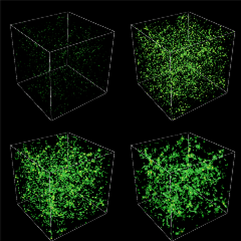
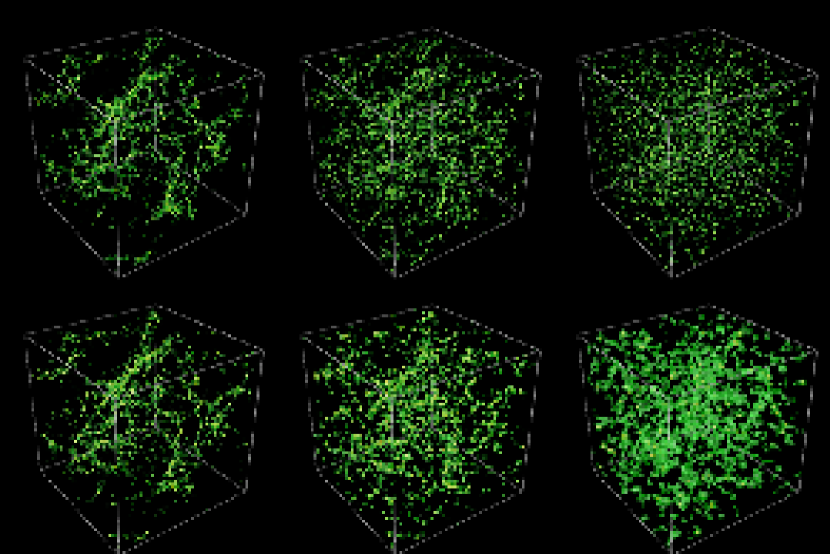
In order to show how clouds form and grow as well as how their distribution evolves, three-dimensional iso-density surfaces at four different times in the S1024 model are presented in Figure 3. As noted above, at the end of the early TI stage ($\sim 4t_{\rm cool}$) mostly small clouds appear. By the end of the follow-up stage of TI and gravitational growth, $\sim 8t_{\rm cool}$, the clouds become larger. During late stage, the clouds become even larger but their number reduces, as a result of cloud-cloud mergers, which can be seen in the bottom two images.

3.2 Identification of Clouds and Their Mass Function

In order to study the properties of formed clouds they were identified using the algorithm CLUMPFIND described by Williams, De Geus & Blitz (1994). The algorithm basically tags cells around a density peak as the “cloud cells”, if they satisfy the prescribed criteria of density and temperature. We chose the following criteria: $\rho\geq 10\rho_{0}$ and $T\leq 10^{5}$K. Here $\rho_{0}$ is the initial mean density. There is an arbitrariness in these threshold values. But the identification of clouds does not depend sensitively on the choices of threshold values, since clouds are well delineated by rather sharp jumps in density and temperature. In addition, we qualified only those with at least $3\times 3\times 3$ cells or more as clouds. Once clouds were identified, their various quantities were calculated.

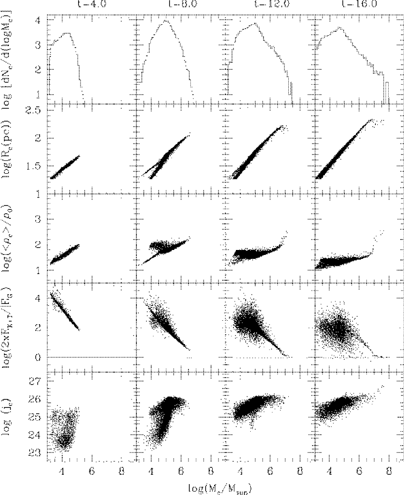
The first row of Figure 4 shows the number of clouds, $N_{c}$, as a function of the cloud mass, $M_{c}$, at the times same as those in Figure 3 in the S1024 model. By $4t_{\rm cool}$ a significant number of clouds, $N_{c}\sim 3\times 10^{3}$, form through the growth of initial high density peaks by TI. The mass function at $4t_{\rm cool}$ is roughly Gaussian, since the initial density perturbations were drown from a random Gaussian distribution. During the follow-up stage of TI and gravitational growth, more peaks develop into clouds and at the same time they become massive. The mass function evolves roughly into the log-normal distribution, shown at $8t_{\rm cool}$. The log-normal distribution is a signature of nonlinear structure formation, as reported in various simulations (see, e.g., Vázquez-Semadeni, 1994; Wada & Norman, 2001). During late stage, more massive clouds develop through gravitational merging as pointed with Figure 3, and so the mass function extends to higher mass. The high mass tail of the mass function beyond the peak follows approximately a power-law distribution. When the mass function is fitted to $dN/dM_{c}\propto M_{c}^{-\alpha}$ for $M_{c}>10^{5.5}~{}{\rm M}_{\sun}$, the value of $\alpha$ decreases from $\sim 0.8$ at $12t_{\rm cool}$ to $\sim 0.6$ at $16t_{\rm cool}$.

3.3 Size, Density and Energetics of Clouds

With the mass, $M_{c}$, and volume, $V_{c}$, of identified clouds, the effective radius was taken as $R_{c}\equiv(3V_{c}/4\pi)^{1/3}$ and the mean density was calculated as $\left<\rho_{c}\right>=M_{c}/V_{c}$. The second and third rows of Figure 4 show $R_{c}$ and $\left<\rho_{c}\right>$ in the S1024 model. For energetics the kinetic energy relative to the cloud’s center of mass, $E_{K}$, the thermal energy, $E_{T}$, and the gravitational energy, $E_{G}$, were calculated for identified clouds. The procedure by which the gravitational energy was calculated is presented in Appendix A along with a note of caution. The fourth row of Figure 4 shows the ratio of positive to negative energies, or the virial parameter

$$\beta\equiv{{2\cdot(E_{K}+E_{T})}\over|E_{G}|}.$$ (11)

The parameter $\beta$ tells whether clouds are primarily pressure-bound ($\beta\gtrsim 2$) or gravitationally bound ($\beta\lesssim 2$). Among the gravitationally bound clouds, the condition $\beta\sim 1$ indicates that they are approximately in virial equilibrium, although, strictly speaking, the condition applies only for a stable system where the external pressure is negligible and the moment of inertia does not change with time.

During the early stage of TI ($\lesssim 4t_{\rm cool}$), as small clumps grow isobarically, their density increases gradually, but $\left<\rho_{c}\right>/\rho_{0}$ has not yet reached the isobaric factor of $\sim(T_{h}/T_{\rm min})\simeq 100$. The self-gravity is negligible with $\beta\gg 2$ during this stage. In the follow-up stage of TI and gravitational growth ($\lesssim 8t_{\rm cool}$), pressure-bound clouds develop fully. Those clouds have roughly $\left<\rho_{c}\right>/\rho_{0}\sim 100$, the maximum isobaric increase from the initial density, and the mean density is a bit higher in clouds with larger mass. Their radius scales roughly as $R_{c}\sim M_{c}^{0.3}$, which can be seen in the second row of Figure 4. The virial parameter has $\beta>2$ for all clouds, confirming that they are still gravitationally unbound. The pressure-bound clouds follow $\beta\propto M_{c}^{-1}$, which can be understood as follows. In those clouds, the thermal energy is dominant over the kinetic energy, i.e., $E_{T}\sim{\rm a~{}few}\times E_{K}$. With $T\sim T_{\rm min}$ in those clouds, the thermal energy scales as $E_{T}\propto M_{c}$. On the other hand, the gravitational energy scales approximately as $E_{G}\propto M_{c}^{2}$, since larger clouds have slightly more concentrated mass distribution.

As clouds grow further primarily through merging in late stage, some of them become massive enough to be gravitationally bound. After that point clouds can be divided into two populations of distinct properties (see the last two times of Figure 4): pressure-bound clouds with smaller mass and gravitationally bound clouds with larger mass. The pressure-bound clouds have the properties similar to those found in the earlier stage. They have mean density $\left<\rho_{c}\right>\sim 100\left<\rho_{bg}\right>$, where $\left<\rho_{bg}\right>$ is the mean background density. Note that the background density continues to decrease as more mass goes to clouds. By the end of the S1024 simulation, $16t_{\rm cool}$, only $\sim 1/4$ of gas mass remains in the background. So the mean density of the pressure-bound clouds decreases with time. Those pressure-bound clouds have $\beta>2$ and follow $\beta\propto M_{c}^{-1}$. The gravitationally bound clouds appear first at $\sim 9t_{\rm cool}$ or $\sim 1.3t_{\rm grav}$ in the S1024 model. In those clouds the self-gravity enhances the density and the mean density of the clouds reaches up to $10^{4}\left<\rho_{bg}\right>$ or even higher by $16t_{\rm cool}$. The fourth raw of Figure 4 shows that the gravitationally bound clouds are approximately in virial equilibrium with $\beta\sim 1$. In addition, we found that in those clouds the kinetic energy is not smaller but sometimes larger than the thermal energy as expected in a virialized system, and both the gravitational energy, $E_{G}$, and the positive energy, $E_{K}+E_{T}$, scale as $M_{c}^{2}$.

Two points are noted on the gravitationally bound clouds. 1) Although these clouds have $\beta\sim 1$, they are not in steady-state. The clouds lose the positive energy rather quickly through cooling and contract further. But at the same time the cloud mass continues to grow through merging. 2) The gravitational energy of these gravitationally bound clouds scales as $E_{G}\propto M_{c}^{2}$, because their radius is in a relatively narrow range of $150-200$ pc regardless of their mass, as shown in the second row of Figure 4. Since there is no physically obvious reason why the clouds with different mass should have similar radii, it should be understood as the result of dynamical evolution. However, their radius is somewhat larger at $16t_{\rm cool}$ than at $12t_{\rm cool}$. This is related to the increase of angular momentum in the clouds with time (see the next subsection).

The distinction between the pressure-bound and gravitationally bound clouds in late stage can be understood with the critical mass

$$M_{\rm crit}=1.18\left(kT_{c}\over\mu m_{H}\right)^{2}G^{-3/2}p_{bg}^{-1/2},$$ (12)

which is the maximum stable mass for an isothermal sphere confined by the background pressure $p_{bg}$ (see e.g., McCrea, 1957; Kang, Lake & Ryu, 2000). For $T_{c}=10^{4}$ K and the background pressure four times smaller than the initial pressure (due to decrease in the background density), the critical mass is $M_{\rm crit}\simeq 6\times 10^{6}~{}{\rm M}_{\sun}$, which coincides well with the transition mass scale in the last two times of Figure 4. Incidentally, this mass is similar to the Jeans mass of clouds, which is given as

$$M_{J}\equiv\rho\lambda_{J}^{3}=6\times 10^{6}\left(T_{c}\over 10^{4}~{}{\rm K}\right)^{3/2}\left(n_{c}\over 100~{}{\rm cm^{-3}}\right)^{-1/2},$$ (13)

where $\lambda_{J}$ is the Jeans length (see e.g., Spitzer, 1979).

Although the simulated model would be too simple to represent a real protogalactic halo, it is tempting to regard the gravitationally bound clouds as possible candidates for PGCCs. That is, some of them may further cool down below $10^{4}~{}{\rm K}$ either by UV self-shielding of H₂ molecules or by self-enrichment of metals due to first generation Type II supernovae, possibly leading to star formation. If about ten of them turn into globular clusters, their number density would be $\sim$ 0.01 clusters/kpc³. However, the typical size of globular clusters $\sim 10$ pc or so. So the clouds should contract further by more than a factor of 10. But the further collapse is controlled by the rotation of clouds (see §3.4 below). In addition, the typical mass of globular clusters is $\sim 10^{6}~{}{\rm M}_{\sun}$ or so. So if these gravitationally bound clouds were to become globular clusters, the star formation efficiency should be $\sim 10\%$ or so with $\sim 90\%$ of their mass dispersed back to protogalactic halo.

It was pointed out by Truelove et al. (1997) that “artificial fragmentation” due to errors arising from discretization occurs in numerical simulations with self-gravity. They argued that the artificial fragmentation can be suppressed if resolution is maintained high enough that, for instance, the “Jeans number” $\Delta l/\lambda_{J}\lesssim 0.25$ or so for isothermal collapses. Here $\lambda_{J}$ is the local Jeans length. We found that although the constraint was not complied in a few high density zones, $\Delta l/\lambda_{J}$ was kept to be always smaller than 0.4 in the S1024 simulation. In any case, we followed only up to the formation of bound clouds, not the subsequent evolution leading to fragmentation of those clouds. So no obvious fragmentation was observed.

3.4 Rotation of Clouds

An important property of clouds that controls the dynamical state and affects the eventual fate is their rotation. To quantify it, the angular momentum of clouds relative to their center of mass, $J_{c}$, was calculated. The bottom row of Figure 4 shows the specific angular momentum of clouds, $j_{c}=J_{c}/M_{c}$, in the S1024 model.

In pressure-bound clouds, rotation plays a minor role in their dynamical evolution, since the rotational energy is smaller by an order of magnitude than the thermal energy. But we found that rotation can be dynamically important in gravitationally bound clouds. The specific angular momentum of those gravitationally bound clouds is larger than that of pressure-bound clouds, which can be seen clearly at $16t_{\rm cool}$. In fact the gravitationally bound clouds with a same $M_{c}$ have higher angular momentum at later time. For example, the clouds with $M_{c}\sim 10^{7.5}~{}{\rm M}_{\sun}$ have a few times larger $j_{c}$ at $16t_{\rm cool}$ than at $12t_{\rm cool}$. This is because the clouds have grown mostly through merging in late stage and they have gained angular momentum through merging as well as tidal torque. Its direct consequence is that the clouds at later stage have larger radius, as noted in the previous subsection. We note that the clouds in our simulations are ever evolving. So it is not meaningful to define the canonical properties of clouds such as $R_{c}$ and $j_{c}$ as a function of $M_{c}$.

The rotation of gravitationally bound objects is often characterized by the dimensionless spin parameter (Peebles, 1969)

$$\lambda_{s}={{J_{c}|E_{G}^{1/2}|}\over{GM_{c}^{5/2}}}.$$ (14)

It measures the degree of rational support of the systems with

$${f_{\rm centrifugal}\over f_{\rm gravity}}\sim{J_{c}\over R_{c}^{3}}{R_{c}^{2}\over GM_{c}}\sim\lambda_{s}^{2}.$$ (15)

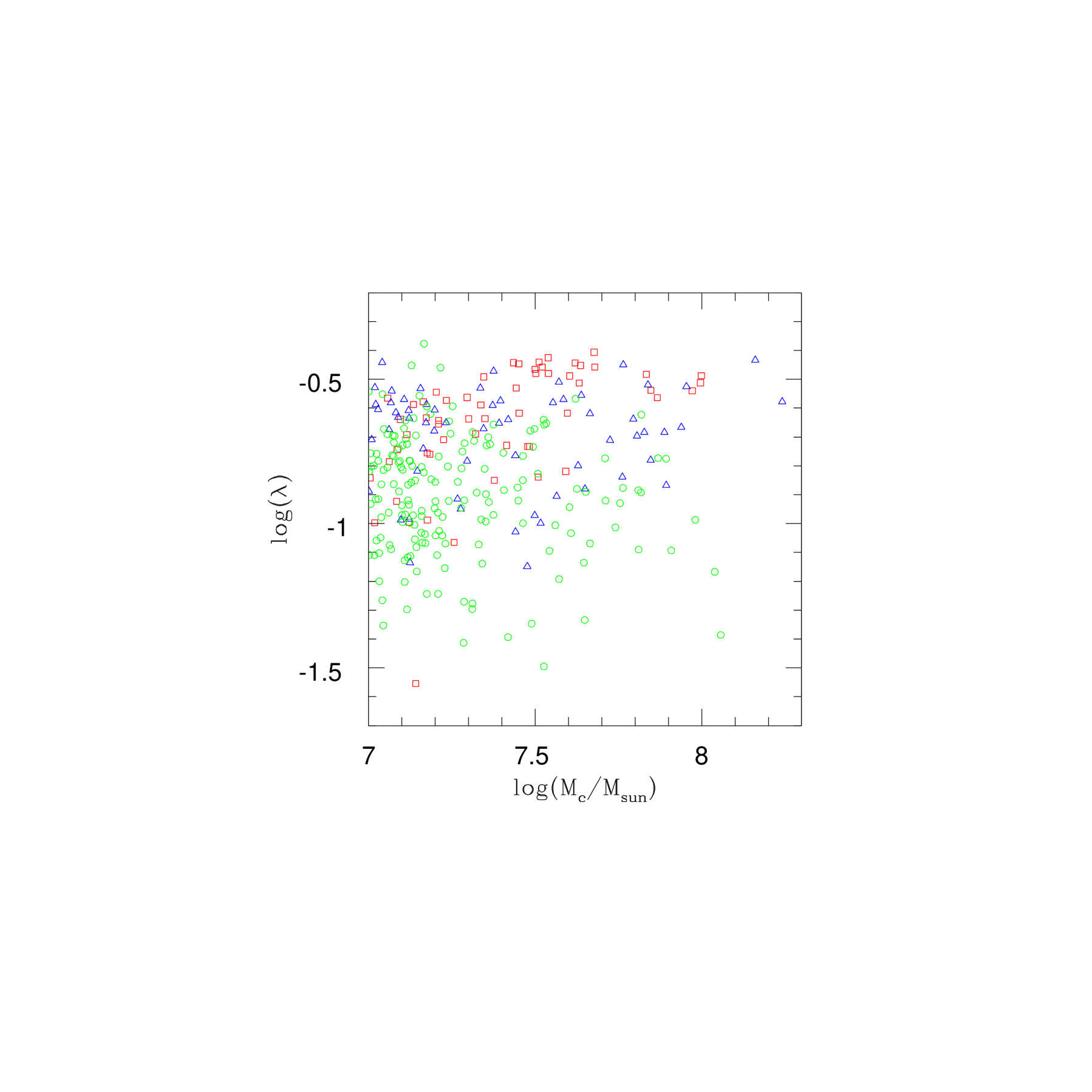
In the context of cosmological $N$-body simulations, it has been shown that the typical value of $\lambda_{s}$ for gravitationally bound objects which acquired angular momentum through gravitational torque is $\sim 0.05$ (e.g., see Barnes & Efstathiou, 1987). In Figure 5 red squares represent the spin parameter for the gravitationally bound clouds with $M_{c}\geq 10^{7}~{}{\rm M}_{\sun}$ at $16t_{\rm cool}$ in the S1024 model. It is clear that $\lambda_{s}$ of our gravitationally bound clouds is significantly larger than 0.05. All except one have $\lambda_{s}>0.05$ and the mean value is $\left<\lambda_{s}\right>\sim 0.3$. It is because the clouds have gained angular momentum through merging as well as torque.

With such large values of $\lambda_{s}$, the degree of rotational support of the gravitationally bound clouds should be already substantial. Hence, rotation should be the key parameter that determines whether some of those clouds could become PGCCs and collapse further to globular clusters. For instance, in a dissipative collapse that conserves angular momentum, the clouds with $\lambda_{s}\sim 0.3$ can contract only by a factor of a few, before they become completely rotationally supported and disk-shaped. However, yet it is not clear whether we should conclude that those clouds with $\lambda_{s}\sim 0.3$ can not evolve into globular clusters. It is because we can not rule out the possibility that the clouds may be able to lose most, say $\sim 99\%$, of their angular momentum, while they collapse and lose $\sim 90\%$ of their mass. For instance, in the so-called self-enrichment model of globular cluster formation, first generation Type II supernovae govern star formation and the removal of residual gas (e.g., see Parmentier et al., 1999; Shustov & Wiebe, 2000). In this model the star formation may have occurred preferentially at the core, and most gas in the outskirt with large angular momentum may have been blown out.

In addition, as noted above, the gravitationally bound clouds found at an earlier time have smaller angular momentum. So if the clouds were detached from background and started to collapse earlier, the angular momentum restriction would be somewhat less severe. Also the clouds emerged from different environments could have smaller angular momentum (for instance, see §3.8). In any case, subsequent evolution of the gravitationally bound clouds is beyond the scope of this paper, so the possible connection between these clouds and PGCCs should be left as a future study.

3.5 Shape of Clouds

Shape is another property of clouds that reflects their dynamical state. In order to quantify it, we examined the shape parameters defined as

$$q\equiv{b\over a}\qquad{\rm and}\qquad s\equiv{c\over a},$$ (16)

with each cloud fitted to triaxial ellipsoid with axes of $a\geq b\geq c$. The shape parameters have been commonly used to study clumps in numerical simulations (e.g., Curir, Diaferio & de Felice, 1993; Gammie & Lin, 2003). In order to find them, first the moment of inertia tensor,

$$I_{ij}=\int\rho x_{i}x_{j}d^{3}{\vec{x}},$$ (17)

was constructed for each cloud. Here $\vec{x}$ is the displacement relative to the cloud’s center of mass and the integral is taken over the cloud volume. Then, from the three eigenvalues of the tensor, $I_{11}\geq I_{22}\geq I_{33}$, the shape parameters were calculated as

$$q=\left({I_{22}\over I_{11}}\right)^{1/2}\qquad{\rm and}\qquad s=\left({I_{33}\over I_{11}}\right)^{1/2}.$$ (18)

The clouds with $s\sim q<1$ are of prolate shape and the clouds with $s<1$ and $q\sim 1$ are of oblate shape, while triaxial clouds have $s<q<1$. Spherical clouds have $s\sim q\sim 1$.

In the previous study of isolated, thermally unstable clouds using two-dimensional simulations in cylindrical geometry, we showed that the cloud shape changes in the course of the evolution (Baek, Kang & Ryu, 2003). The degree of oblateness or prolateness is enhanced during the initial cooling phase, as expected. But it can be reversed later due to the supersonic infall along the direction perpendicular to the initial flatness or elongation.

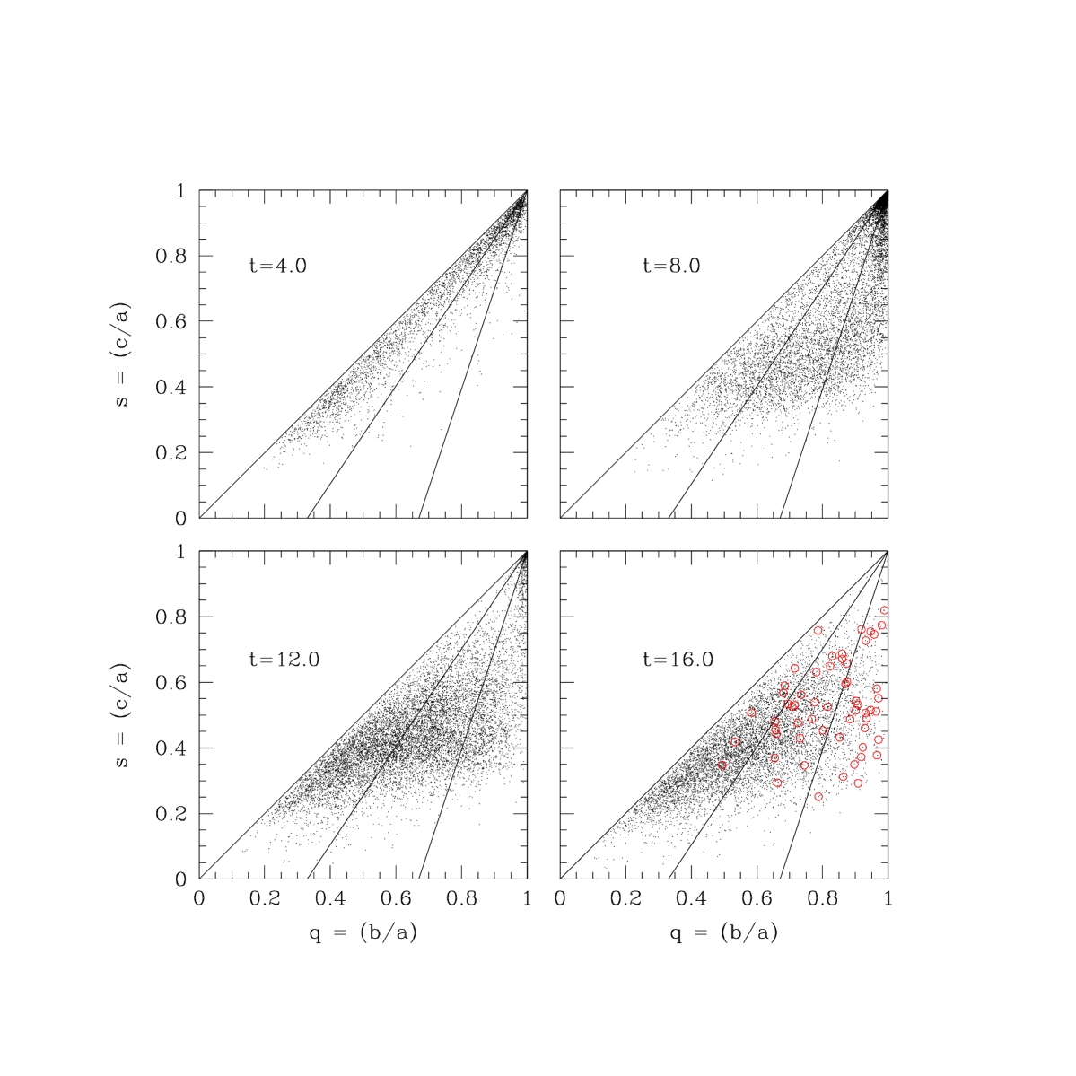
In Figure 6 dots represent clouds in the $q-s$ plane at four times in the S1024 model. Lines divide the domain into three regions of roughly prolate (left), triaxial (middle) and oblate (right) shapes. The panel for $4t_{\rm cool}$ indicates that most clouds formed as a result of TI at early stage are preferentially of prolate shape. This is can be understood from the fact that filaments are the morphology dominant next to knots of clouds. By $8t_{\rm cool}$ some of prolate clouds have been transformed to be oblate, as the result of the shape reversal, which was observed in the two-dimensional study. However, the figure shows that in late stage clouds tend to shift back to be prolate again. This is because gravitational merging results preferentially in clouds of elongated prolate shape.

The gravitationally bound clouds with $M_{c}\geq 10^{7}~{}{\rm M}_{\sun}$, shown in Figure 5, are marked with red circles in the panel for $16t_{\rm cool}$. It is interesting to note that unlike most clouds, those massive clouds are preferentially of oblate shape. It is because those clouds have large angular momentum and a substantial degree of rational support.

3.6 Numerical Convergence

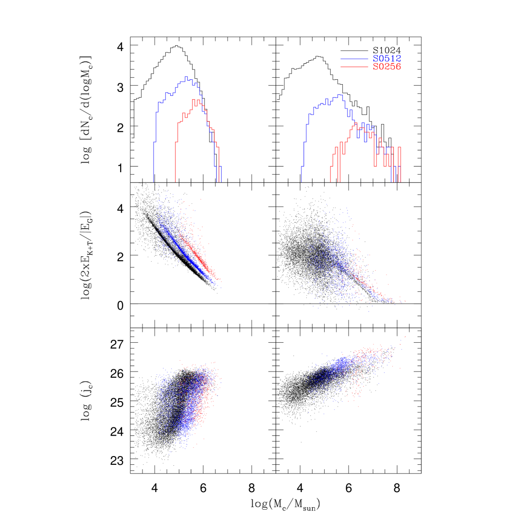
Convergence is an important issue in any numerical simulations. We tested it by comparing the results of simulations with different resolution, i.e., S1024, S0512 and S0256 models (see Table 1). Figure 7 shows the density power spectrum of the S0512 and S0256 models, which can compared with that of the S1024 model in Figure 2. Note that in our simulations the amplitude of the initial power spectrum was set by the condition

$$\int_{\rm all}P_{k}dk\equiv A\int_{\rm all}k^{n}dk=(1+\delta_{\rm rms}^{2})\left<\rho\right>^{2}$$ (19)

with $\delta_{\rm rms}=0.2$ for all resolutions. Simulations with different resolution covers different range of wavenumbers. So the simulations of lower resolution started with larger amplitude, as shown in the figure. Otherwise, the evolution of the power spectrum looks similar in all three models. For instance, the two most noticeable features in Figure 2, i.e., the initial decrease and follow-up fast growth of small scale powers, are also present in Figure 7. But an interesting point is that the scale that suffered the initial decrease is insensitive to resolution, because it was caused by smoothing due traveling sound waves. On the other hand, the scale of the peak in the power spectrum after the follow-up fast growth does depend on resolution. As a matter of fact, the peak at $4t_{\rm cool}$ in the S0256 model occurs at the scale almost four times larger than in the S1024 model. This indicates that the small scale growth in our simulations was limited by resolution, as expected.

Figure 8 shows the mass function, virial parameter and specific angular momentum of clouds in the three models. The left panels show the results at early TI stage, while the right panels show the results at late merging stage. For early stage a different time was chosen for each model so that the density power spectrum has a similar amplitude. In late stage, however, the differences caused by the initial amplitude of power spectrum become insignificant, so $15~{}t_{\rm cool}$ is chosen for all three models. We see that the mass function have been converged for massive clouds, i.e., those with $M_{c}\gtrsim 10^{6}~{}{\rm M}_{\sun}$ at the early stage and those with $M_{c}\gtrsim 10^{7}~{}{\rm M}_{\sun}$ at $15~{}t_{\rm cool}$. However, the number of smaller mass clouds depends on numerical resolution, as expected. With the minimum number of $3^{3}$ zones for identified clouds, the minimum mass scales $M_{\rm min}\propto(\Delta l)^{3}$. On the contrary, at the early stage the virial parameter is larger in lower resolutions for clouds of all mass. It is because the clouds are less compact in lower resolution, and so their gravitational energy is smaller. But as the clouds grow more massive and larger in late stage, the difference in the virial parameter becomes smaller. The angular momentum of clouds is somewhat smaller in lower resolution at the early stage. It is partly because the time of the plot is different in different models. However, in late stage the angular momentum becomes comparable in all three models.

Overall, the formation of small mass clouds, initially through TI and subsequently by compression and infall, was affected by resolution in our simulations. However, we found that the massive, gravitationally bound clouds, which have formed mostly through gravitational merging, have the properties which are almost converged.

3.7 Effects of Initial Power Spectrum

The effects of different initial perturbations on the formation and evolution of clouds were examined by comparing the results of simulations with different initial density power spectrum, i.e., the K0512 and R0512 models, to those of the S0512 model (see Table 1). The K0512 model started with more power on larger scales, while the R0512 model started with more power on smaller scales. Figure 9 shows the density power spectrum of the K0512 and R0512 models. In both models, small scale powers suffered the initial decrease, as in the S0512 model. Especially most of the powers in $k\gtrsim 40$ were erased substantially in the R0512 model. Hence, the overall growth was delayed in the R0512 model. On the other hand, the growth proceeded faster in the K0512 model, with more powers on large scales in the beginning.

Figure 10 shows the total number of clouds as a function of time in the three models with different initial density power spectrum. The overall evolution is similar; the number of clouds increases during the TI and follow-up growth stages, but eventually decreases as gravitational merging progresses. But as noted above, the K0512 model evolves first and the S0512 and R0512 models follow. So clouds form from $t\sim 2t_{\rm cool}$ in K0512, from $t\sim 5t_{\rm cool}$ in S0512 and from $t\sim 10t_{\rm cool}$ in R0512. However, an interesting point is that the maximum number of clouds is about the same with $N_{\max}\sim 3000$ in all three models.

In Figure 11 three-dimensional iso-density surfaces are plotted at two sets of times in the three models. Different times were chosen in different models, since the formation and evolution of clouds proceeds differently. The upper panels show the surfaces when the number of clouds is highest, i.e., at $3t_{\rm cool}$ for K0512, $6t_{\rm cool}$ for S0512 and $11t_{\rm cool}$ for R0512. The lower panels show the surfaces after the number of clouds have decreased a little bit due to merging, i.e., at $4t_{\rm cool}$ for K0512, at $10t_{\rm cool}$ for S0512 and at $19t_{\rm cool}$ for R0512. The most noticeable feature is that the distribution is more “filamentary” in the K0512 model, but less “filamentary” in the R0512 model, than in the S0512 model. It is because that the initial large scale powers, which were largest in the K0512 model but almost absent in the R0512 model, have been developed into significant coherent structures in the cloud distribution.

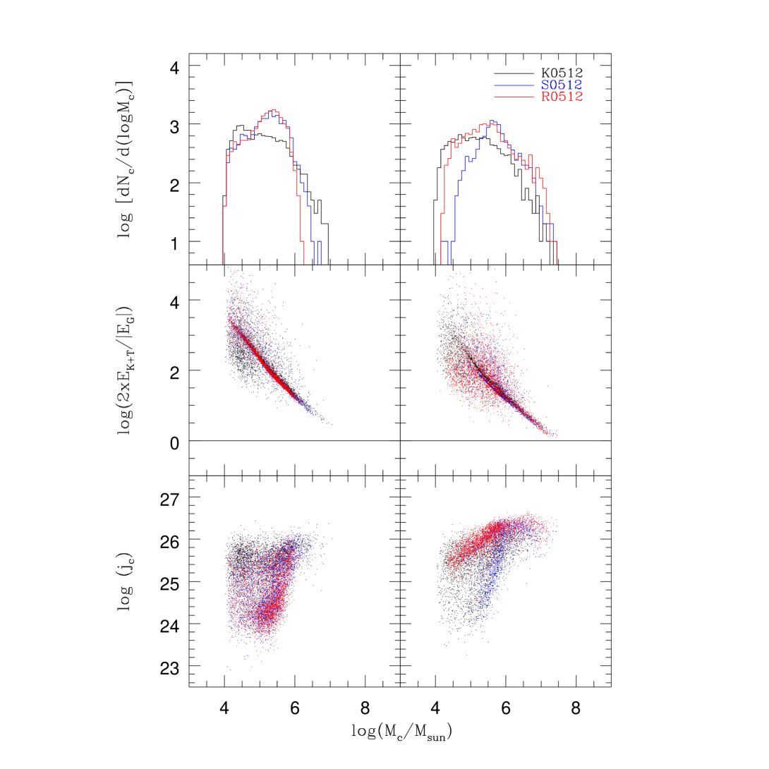
Figure 12 shows the mass function, virial parameter and specific angular momentum of clouds in the three models. The same two sets of times as those in Figure 11 were chosen. Clouds in the K0512 (R0512) model are slightly more (less) massive in the left panels and slightly less (more) massive in the right panels. However, considering the difference in the plotted time, the cloud mass function should be regarded as reasonably similar in the three models. On the other hand, the virial parameter of pressure-bound clouds follows the same diagonal strip in all three models. There is a spread in the distribution of angular momentum, again partly because the plotted time is different in different models. But the angular momentum of the clouds in high mass tail is similar. So we conclude that the properties of individual clouds, especially for massive clouds, are not sensitive to the initial perturbations, while the spatial distribution of clouds reflects the slope of initial density power spectrum.

3.8 Effects of Different Density and Cooling

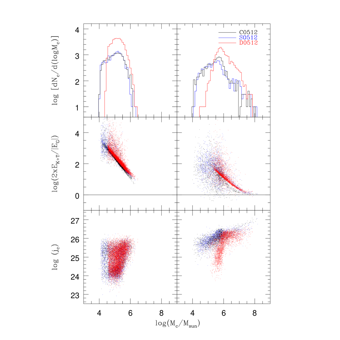
The effects of gas density on the formation and evolution of clouds were examined with the D0512 model, which has the background density 3 times larger than that of the S0512 mode. Otherwise the two models are identical (see Table 1). With $t_{\rm cool}/t_{\rm grav}\propto n_{h}^{-1/2}$, the gravity is relatively less important in the D0512 model. Figure 13 compares the mass function, virial parameter and specific angular momentum of clouds in the D0512 model (red lines and dotes) with those in the S0512 model at an early stage of TI ($5t_{\rm cool}$) and at a late stage of merging ($15t_{\rm cool}$), respectively. In the D0512 model there are more clouds with larger mass, reflecting the higher background density. Yet, the virial parameter is almost identical in the two models, indicating that the background density is not important in determining the energetics of individual clouds. As a matter of fact, we found that the properties of clouds, except the angular momentum, are not sensitive to the background density. The angular momentum of the clouds identified in the early stage of TI is similar in the two models. But in late stage the angular momentum is noticeably smaller in the higher background density model. The same trend is also obvious in the spin parameter of gravitationally bound clouds, which is shown for $M_{c}\geq 10^{7}~{}{\rm M}_{\sun}$ in Figure 5. While the spin parameter for the S0512 model (blue triangles) does not differ much from that for the higher resolution S1024 model (red squares), the spin parameter for the D0512 model (green circles) is substantially smaller with the median value of $\lambda_{\rm med}\sim 0.12$. This is because the clouds formed in higher background density have experienced relatively less tidal torque and gravitational merging, through which they have acquired angular momentum.

The effects of possible cooling further below $10^{4}~{}{\rm K}$ were examined with the C0512 model, which includes a mock ${\rm H_{2}}~{}$cooling given in equation (7). Otherwise it is same as the S0512 model (see Table 1). Figure 13 compares the mass function, virial parameter and specific angular momentum of clouds in the C0512 model (black lines and dotes) with those in the S0512 model. The cloud properties are similar overall, except the smaller thermal energy in the C0512 model, which is expected from the additional cooling. Because the thermal energy counts for most of the positive energy, especially in pressure-bound clouds, the virial parameter is smaller in the C0512 model. But in massive, gravitational bound clouds, the kinetic energy is comparable to or sometimes larger than the thermal energy, as noted in §3.3. So the effects of the additional cooling is less important in those clouds.

To quantify how much the additional cooling changes the thermal state of gas, we compare the mass distribution, $f(T)$, for the S0512 and C0512 models in Figure 14. The gas with $T\sim 10^{4}~{}{\rm K}$ in S0512 spreads below $10^{4}~{}{\rm K}$ in C0512, as expected. In addition some of the gas with $10^{4}\lesssim T\lesssim 2\times 10^{4}~{}{\rm K}$ has cooled below $10^{4}~{}{\rm K}$. But the additional cooling does not affect much the gas of higher temperature. Even with this additional cooling the mass fraction peaks still at $T\sim 1.5\times 10^{4}~{}{\rm K}$ and most of the “cloud gas” has $10^{3}\lesssim T\lesssim 10^{5}~{}{\rm K}$, not only because the assumed mock ${\rm H_{2}}~{}$cooling is inefficient, but also because some of the gas has been reheated by shocks and compression.

Here we should note that with lower temperature, the clouds in the C0512 model have smaller Jeans mass and could go through further fragmentation. But with a fixed grid resolution, the simulation could not follow it. In fact, in the C0512 model, the Jeans number, $\Delta l/\lambda_{J}$, reached up to $\gtrsim 1$ in the center of some gravitationally bound clouds. However, as noted above, we did not intend to follow such fragmentation in this study.

4 Summary and Discussion

We study the role of self-gravity and gravitational interactions in the formation of clouds via thermal instability (TI) through three-dimensional hydrodynamic simulations. We considered the gas in protogalactic halo environment with $T\sim 1.7\times 10^{6}$K and $n\sim 0.1~{}{\rm cm^{-3}}$ in a periodic box of 10 kpc and followed its evolution for up to 20 cooling time. We adopted idealized models in which a static, non-magnetized gas cools radiatively with initial isothermal density perturbations. A radiative cooling rate in ionization equilibrium for an optically thin gas with the primordial composition was used. In addition, an ad hot heating was included, which emulates feedbacks from stellar winds, supernovae, turbulence and shocks in order to maintain the thermal balance of background gas.

The main results can be summarized as follows: 1) Clouds form first on scales much smaller than the cooling length as a result of non-linear behavior of TI. 2) Those small clouds grow through compression by background pressure as well as gravitational infall, but eventually they merge by gravity to become gravitationally bound objects. 3) The gravitationally bound clouds have acquired angular momentum through merging as well as tidal torque. So they have high angular momentum with the spin parameter of $\left<\lambda_{s}\right>\sim 0.3$ or so. 4) The spatial distribution of clouds depends on initial perturbations, for instance, the slope of initial density power spectrum, but the properties of individual clouds are not sensitive to that.

We note that the realistic picture of thermal-gravitational instability that in protogalactic halos should be more complex than in the numerical models considered here. Some of key aspects include: 1) The gas in real protogalactic halos is likely in a chaotic state induced during the formation of halos themselves. The chaotic flow motions would have suppressed the early formation of clouds via TI, but increased collisions of clouds once formed. 2) Protogalactic halos have their own structures, but the effects of those structures were ignored. For instance, the tidal torque exerted by the halo and/or the rotation in disk would have suppressed the formation of clouds. 3) There are emerging evidences that magnetic field existed even in the early galaxies where the oldest stars formed (see, e.g., Zweibel, 2003). Then, undoubtedly the magnetic field should have affected the formation and properties of clouds profoundly. 4) It is well known that when a hot gas cools from $T>10^{6}$ K, it recombines out of ionization equilibrium because the cooling time scale is shorter than the recombination time scale (Shapiro & Kang, 1987). However, details of the cooling such as non-equilibrium ionization and ${\rm H_{2}}~{}$and metal cooling below $10^{4}$K could have only minor effects on our main conclusions.

Although the numerical models are rather idealized to facilitate simulations, our results should provide crude insights on the formation of PGCCs in protogalactic halos. The gravitationally bound clouds in our simulations have mass $M_{c}\gtrsim 10^{7}~{}{\rm M}_{\sun}$ and radius $R_{c}\simeq 150-200$ pc. If some of them evolved into PGCCs and became globular clusters, they should have lost $\sim 90\%$ of their mass with $\sim 10\%$ of star formation efficiency, and at the same time they should have collapsed by a factor 10 or so. But the further collapse would not have been straightforward because of large angular momentum, unless their angular momentum was removed very efficiently along with mass during the star formation phase. Such removal of angular momentum may not be impossible, but following it is beyond the scope of this numerical study. It should be studied with simulations that have resolution high enough to follow the fragmentation of clouds and the subsequent formation of stars inside PGCCs. However, we make the following note of caution. The clouds in our simulations continue to grow mostly through merging in late stage, and thus their mass and angular momentum increase in time. So any simulations of isolated clouds to study the ensuing evolution of PGCCs could be misleading.

We should point that there is a caveat in our argument for the large angular momentum of gravitationally bound clouds. The angular momentum was acquired mostly through gravitational processes, i.e., tidal torque and merging. So if the clouds formed in an environment where the gravitational processes are less important, they would have acquired less angular momentum. For instance, we showed that the clouds formed in a denser background have smaller angular momentum. Hence, if protogalactic halos consisted of smaller halo-lets and clouds formed in shocked regions after collisions of halo-lets, as suggested by e.g., Gunn (1980), they could have smaller angular momentum.

Appendix A Corrected Potential

In our simulations, the gravitational potential for the gas-dynamical equation in §2.2 was calculated by using the FFT method, $\Phi_{\rm FFT}(\vec{r})$. Then the gravitational force could be correctly calculated by differentiating this potential on the grid. However the use of $\Phi_{\rm FFT}(\vec{r})$ in calculating the gravitational energy of clouds, $E_{G}$, in §3.3 ends up a large error, because $\Phi_{\rm FFT}(\vec{r})$ is undetermined by an integral constant. In principle, the gravitational potential of isolated clouds can be precisely calculated by the direct double integration over cloud volume. However, the computational cost of this method is prohibitively expensive, especially for gravitationally bound clouds in the $1024^{3}$ simulation, since they occupy typically $\sim 10^{4}$ or so grid zones. One the other hand, the direct integration does not take account of contributions from the rest of mass in the simulation box as well as the periodic mass distribution. But we found that those contributions are small, especially for massive, gravitationally bound clouds.

As an effort to estimate the gravitational energy of clouds more accurately, we devised a method which calculates and uses the corrected potential as follows:
1) The position, $\vec{r}_{\rm min}$, where $\Phi_{\rm FFT}(\vec{r})$ has the minimum value, is found for each cloud, and then the potential at the position is calculated by the direct integration,

$$\Phi_{\rm direct}(\vec{r}_{\rm min})=-G\int{{\rho({\vec{r^{\prime}}})}\over{|{\vec{r^{\prime}}}-\vec{r}_{\rm min}|}}dV^{\prime}.$$ (A1)

2) The difference between $\Phi_{\rm direct}$ and $\Phi_{\rm FFT}$ at $\vec{r}_{\rm min}$ is calculated for each cloud,

$$C=\Phi_{\rm direct}(\vec{r}_{\rm min})-\Phi_{\rm FFT}(\vec{r}_{\rm min}).$$ (A2)

3) Then the corrected potential for each cloud is calculated by

$$\Phi_{\rm corr}(\vec{r})=\Phi_{\rm FFT}(\vec{r})+C.$$ (A3)

4) Finally the gravitation energy of each cloud is calculated as

$$E_{G}=\int{1\over 2}\rho(\vec{r})\Phi_{\rm corr}(\vec{r})dV.$$ (A4)

Figure 15 demonstrates the motivation of our effort. Here $E_{\rm N^{2}}$ is the gravitational energy of clouds calculated by the direct double integration, while $E_{\rm FFT}$ and $E_{\rm corr}$ were calculated using $\Phi_{\rm FFT}$ and $\Phi_{\rm corr}$, respectively. The errors for the S0256 model are shown, where the double integration could be done with a reasonable computation time. $E_{\rm corr}$ tends to agree with $E_{\rm N^{2}}$ better than $E_{\rm FFT}$. With $E_{\rm corr}$ the error is within $\sim 20\%$ or so for a substantial fraction of clouds. However, the estimation of gravitational energy could be easily off by a factor two or even larger with $E_{\rm FFT}$. We used $E_{\rm corr}$ for the gravitational energy in §3.3.

Table 1: Model Parameters for Simulations

Model	No. of grid zones	$t_{\rm end}$ ($t_{\rm cool}$)	$t_{\rm end}$ ($t_{\rm grav}$)	$T_{\rm min}$ (K)	$P_{k}$	$n_{h}$ (${\rm cm}^{-3}$)
S1024	$1024^{3}$	16	2.29	$10^{4}$	const	0.1
S0512	$512^{3}$	20	2.86	$10^{4}$	const	0.1
S0256	$256^{3}$	20	2.86	$10^{4}$	const	0.1
K0512	$512^{3}$	20	2.86	$10^{4}$	$\propto k^{-{5\over 3}}$	0.1
R0512	$512^{3}$	20	2.86	$10^{4}$	$\propto k^{2}$	0.1
C0512	$512^{3}$	20	2.86	$10^{2}$	const	0.1
D0512	$512^{3}$	20	1.65	$10^{4}$	const	0.3

Figure 1: Cooling function, $L(T)\equiv\Lambda/n_{H}^{2}$, of the collisional ionization equilibrium (CIE) cooling for a gas with zero-metalicity (solid line). The dotted line is for the mock ${\rm H_{2}}~{}$cooling adopted in Model C.

Figure 2: Evolution of the density power spectrum in the S1024 model. Dots represent the initial power spectrum at $t=0$ and lines are the power spectrum at $t_{\rm cool}$, $2~{}t_{\rm cool}$, $3~{}t_{\rm cool}$, $\ldots$, $16~{}t_{\rm cool}$.

Figure 3: Iso-density surfaces inside the full simulation box of size $10~{}{\rm kpc}$ at $4~{}t_{\rm cool}$ (top-left), $8~{}t_{\rm cool}$ (top-right), $12~{}t_{\rm cool}$ (bottom-left), and $16~{}t_{\rm cool}$ (bottom-right) in the S1024 model. Green surfaces corresponds to $10\rho_{0}$, yellow surfaces corresponds to $10^{2}\rho_{0}$ and red surfaces corresponds to $10^{3}\rho_{0}$. Here $\rho_{0}$ is the mean initial density.

Figure 4: Differential number of clouds, $dN_{c}/d(\log M_{c})$, effective radius, $R_{c}$, mean density, $\left<\rho\right>_{c}$, energy ratio, $2(E_{T}+E_{K})/|E_{G}|$, and specific angular momentum, $j_{c}$, as a function of cloud mass, $M_{c}$, at four different times in the S1024 model. Here, $j_{c}$ is in the cgs units

Figure 5: Spin parameter, $\lambda_{s}={{J|E_{G}^{1/2}|}/{GM^{5/2}}}$, as a function of cloud mass, $M_{c}$, for clouds with $M_{c}\geq 10^{7}~{}{\rm M}_{\sun}$. Red squares are for the S1024 model, blue triangles are for the S0512 model, and green circles are for the D0512 model at $16~{}t_{\rm cool}$.

Figure 6: Shape parameters, $q=b/a$ and $s=c/a$, at four different times in the S1024 model. The principal axes of clouds are defined such that $a\geq b\geq c$. The domain is divided into three regions containing the clouds of prolate shape ($s\sim q<1$, left), and the clouds of oblate shape ($s<1$ and $q\sim 1$, right) and the clouds of triaxial shape ($s<q<1$, middle). Red circles represent the clouds with $M_{c}\geq 10^{7}~{}{\rm M}_{\sun}$.

Figure 7: Evolution of the density power spectrum in the S0256 and S0512 models. Dots represent the initial power spectrum at $t=0$ and lines are the power spectrum at $t_{\rm cool}$, $2~{}t_{\rm cool}$, $3~{}t_{\rm cool}$, $\ldots$, $20~{}t_{\rm cool}$.

Figure 8: Differential number of clouds, $dN_{c}/d(\log M_{c})$, energy ratio, $2(E_{T}+E_{K})/|E_{G}|$, and specific angular momentum, $j_{c}$, as a function of cloud mass, $M_{c}$, in the three models with different resolution. Left panels show the quantities at $5~{}t_{\rm cool}$, $6~{}t_{\rm cool}$, and $7~{}t_{\rm cool}$ for the S0256, S0512, and S1024 models, respectively, and right panels show the quantities at $15~{}t_{\rm cool}$ for all three models. Here, $j_{c}$ is in the cgs units.

Figure 9: Evolution of the density power spectrum in the K0512 and R0512 models. Dots represent the initial power spectrum at $t=0$ and lines are the power spectrum at $t_{\rm cool}$, $2~{}t_{\rm cool}$, $3~{}t_{\rm cool}$, $\ldots$, $20~{}t_{\rm cool}$.

Figure 10: Time evolution of the number of clouds, $N_{c}$, in the three models with different initial density power spectrum.

Figure 11: Iso-density surfaces inside the full simulation box of size $10~{}{\rm kpc}$ in the K0512 model (left images), in the S0512 model (middle images), and in the R0512 model (right images). Top images are at $3~{}t_{\rm cool}$ in the K0512 model, at $6~{}t_{\rm cool}$ in the S0512 model, and at $11~{}t_{\rm cool}$ in R0512 model. Lower images are at $4~{}t_{\rm cool}$ in the K0512 model, at $10~{}t_{\rm cool}$ in the S0512 model, and at $19~{}t_{\rm cool}$ in the R0512 model. Green surfaces corresponds to $10\rho_{0}$, yellow surfaces corresponds to $10^{2}\rho_{0}$ and red surfaces corresponds to $10^{3}\rho_{0}$, same as in Figure 3.

Figure 12: Differential number of clouds, $dN_{c}/d(\log M_{c})$, energy ratio, $2(E_{T}+E_{K})/|E_{G}|$, and specific angular momentum, $j_{c}$, as a function of cloud mass, $M_{c}$, in the three models with different initial density power spectrum. Left panels are at $3~{}t_{\rm cool}$, $6~{}t_{\rm cool}$, and $11~{}t_{\rm cool}$ for the K0512, S0512, and R0512 models, respectively, and right panels are at $4~{}t_{\rm cool}$, $10~{}t_{\rm cool}$, and $19~{}t_{\rm cool}$ for the K0512, S0512, and R0512 models, respectively. Here, $j_{c}$ is in the cgs units.

Figure 13: Differential number of clouds, $dN_{c}/d(\log M_{c})$, energy ratio, $2(E_{T}+E_{K})/|E_{G}|$, and specific angular momentum, $j_{c}$, as a function of cloud mass, $M_{c}$, in the C0512 and D0512 models as well as in the S0512 model for comparison. Left panels are at $5~{}t_{\rm cool}$, and right panels are at $15~{}t_{\rm cool}$, respectively, for all three models. Here, $j_{c}$ is in the cgs units.

Figure 14: Mass fraction, $f(T)$, of gas as a function of temperature at three different times in the S0512 and C0512 models.

Figure 15: Error in the estimation of gravitational energy by the FFT potential (bottom panels) and the corrected potential (top panels) at $10~{}t_{\rm cool}$ (left panels) and $15~{}t_{\rm cool}$ (right panels) in the S0256 model. See the Appendix A for details.

References

- Baek, Kang & Ryu (2003) Baek, C. H., Kang, H. & Ryu, D., 2003, ApJ, 584, 675
- Balbus (1986) Balbus, S. A. 1986, ApJ, 303, L79
- Barnes & Efstathiou (1987) Barnes, J. & Efstathiou, G. 1987, ApJ, 319, 575
- Brinkman, Massaglia & Müller (1990) Brinkman, W., Massaglia, S. & Müller, E.1990, A&A, 237, 536
- Burkert & Lin (2000) Burkert, A. & Lin, D. N. C. 2000, ApJ, 537, 270
- Chandran & Cowley (1998) Chandran, B. D. G. & Cowley, S. C. 1998, Phys. Rev. Lett., 80, 3077
- Curir, Diaferio & de Felice (1993) Curir, A., Diaferio, A. & de Felice, F. 1993, ApJ, 413, 70
- David, Bregman & Seab (1988) David, L. P., Bregman, J. N. & Seab, C. G. 1988, ApJ, 329, 488
- Fall & Rees (1985) Fall, S. M. & Rees J. M. 1985, ApJ, 298, 18
- Field (1965) Field, G. B. 1965, ApJ, 142, 531
- Field, Goldsmith & Habing (1969) Field, G. B., Goldsmith, D. W. & Habing, H. J. 1969, ApJ, 142, 531
- Gammie & Lin (2003) Gammie, C. F. & Lin, Y. T. 2003, ApJ, 592, 203
- Gunn (1980) Gunn, J.E. 1980, in Globular Clusters, ed. D. Hanes & G. Madore, (Cambridge: Cambridge University Press), p. 301.
- Kang, Lake & Ryu (2000) Kang, H., Lake, G. & Ryu, D. 2000, Journal of Korean Astrophysical Society, 33, 111
- Koyama & Inutsuka (2002) Koyama, H. & Inutsuka, S. 2002, ApJ, 564, L97
- Koyama & Inutsuka (2004) Koyama, H. & Inutsuka, S. 2004, ApJ, 602, L25
- Kravtsov & Gnedin (2005) Kravtsov, A. V. & Gnedin, O. Y. 2005, ApJ, 623, 650
- Malagoli, Rosner & Fryxell (1990) Malagoli, A., Rosner, R. & Fryxell, B. 1990, MNRAS, 247, 367
- Kritsuk & Norman (2002) Kritsuk, A. G. & Norman, M. L. 2002, ApJ, 569, L127
- McCrea (1957) McCrea, W. H. 1957, MNRAS, 117, 562
- McKee & Begelman (1990) McKee, C. F. & Begelman, M. C. 1990, ApJ, 358, 392
- McKee & Ostriker (1977) McKee, C. F. & Ostriker, J. P. 1977, ApJ, 218, 148
- Nulsen (1986) Nulsen, P. E. J. 1986, MNRAS. 221, 377
- Parmentier et al. (1999) Parmentier, G., Jehin, E., Magain, P., Neuforge, C., Noels, A.& Thoul, A. A. 1999, A&A, 352, 138
- Peebles (1969) Peebles, P. J. E. 1969, ApJ, 155, 393
- Ryu et al. (1993) Ryu, D., Ostriker, J. P., Kang, H. & Cen, R. 1993, ApJ, 414, 1
- Shapiro & Kang (1987) Shapiro, P. R. & Kang, H. 1987, ApJ, 318, 32
- Shustov & Wiebe (2000) Shustov, B. M. & Wiebe, D. S. 2000, MNRAS, 319, 1047
- Spitzer (1979) Spitzer, L. Jr. 1979, Physical Processes in the Interstellar Medium, (New York: Wiley-Interscience)
- Sutherland & Dopita (1993) Sutherland, R, S. & Dopita, M, A. 1993, ApJS, 88, 253
- Truelove et al. (1997) Truelove, J. K., Klein, R. I., McKee, C. F., Holliman II, J. H., Howell, L. H. & Greenough, J. A. 1997 ApJ, 489, L197
- Vázquez-Semadeni (1994) Vázquez-Semadeni, E. 1994, ApJ, 423, 681
- Wada & Norman (2001) Wada, K. & Norman, C. A. 2001, ApJ, 547, 172
- Williams, De Geus & Blitz (1994) Williams, J.P., De Geus, E. J. & Blitz, L. 1994, ApJ, 428, 693
- Zweibel (2003) Zweibel, E. G. 2003, ApJ, 587, 625