Wide-Angle Wind Driven Bipolar Outflows: High Resolution Models with Application to Source I of the Becklin-Neugebauer / Kleinmann-Low OMC-I Region

Abstract

We carry out high resolution simulations of the inner regions of a wide angle wind driven bipolar outflow using an Adaptive Mesh Refinement code. Our code follows H-He gas with molecular, atomic and ionic components and the associated time dependent molecular chemistry and ionization dynamics with radiative cooling. Our simulations explore the nature of the outflow when a spherical wind expands into a rotating, collapsing envelope. We compare with key observational properties of the outflow system of Source I in the BN/KL region.

Our calculations show that the wind evacuates a bipolar outflow cavity in the infalling envelope. We find the head of the outflow to be unstable and that it rapidly fragments into clumps. We resolve the dynamics of the strong shear layer which defines the side walls of the cavity. We conjecture that this layer is the likely site of maser emission and examine its morphology and rotational properties. The shell of swept up ambient gas that delineates the cavity edge retains its angular momentum. This rotation is roughly consistent with that observed in the Source I $SiO$ maser spots. The observed proper motions and line-of-sight velocity are approximately reproduced by the model. The cavity shell at the base of the flow assumes an X-shaped morphology which is also consistent with Source I. We conclude that the wide opening angle of the outflow is evidence that a wide-angle wind drives the Source I outflow and not a collimated jet.

1 Introduction

Bipolar outflows are recognized as a fundamental component of the star formation process for low and intermediate mass stars. The precise nature of these outflows has received considerable attention and their observational properties have been well characterized (Richer et al. (2000)). The nature of the mechanisms driving the outflows has not, however, been determined. While there is now a consensus that the outflow is made up of swept-up ambient material driven by a “wind” from the central source (a proto-star or young star) there remains a debate over the form such a wind will take. In some models the star produces a well collimated jet on small scales ($<10~{}AU$) due (most likely) to the action of an accretion disk (Konigl & Pudritz (2000)). Other models assume that the proto-stellar wind is not as strongly collimated taking the form of a “wide-angle wind” (WAW). In many models the WAW will have a momentum distribution such that wind has dense core in the polar direction surrounded by less dense flow at lower latitudes (Shu et al. (2000)). Thus WAWs are often envisioned as having a jet-like component. The distinction between these models plays an important role in the debate about star formation because the nature of the WAW/jet is tied to the nature of the wind launching mechanism at the base. Understanding how winds are driven from an accretion disk (most likely via a coupling of magnetic fields and rotation) is a problem of great importance both because jets/winds are ubiquitous in astrophysical environments and because these flows may carry away a significant fraction of the disk’s angular momentum (Konigl & Pudritz (2000)). Thus the distinction between tightly collimated jets and wide-angle winds informs the debate about the nature of jet launching and accretion disk physics. Since it is difficult to directly observe the wind launching regions (see Woitas et al. (2005) ), the properties of large scale bipolar outflows can aid in understanding the nature of their initial conditions.

In addition to questions concerning the nature of the driving winds, bipolar outflows may play an important role in modifying their natal environments. The energy and momentum budgets associated with the aggregate of outflows in a young cluster can be large enough to either power turbulence in the cloud from which the cluster was born or, in some cases, unbind some fraction of the cloud material (Arce (2003)). Observational and theoretical studies have yet to address this issue in its full complexity and so the role of outflows as environmental factors determining cloud properties remains unclear. Recent studies of the NGC 1333 region have shown that fossil bipolar outflows or “cavities” which remain after the central source has turned off provide a significant coupling agent linking wind momenta to the cloud (Quillen et al. (2004)). This work emphasizes the importance of understanding outflow properties in terms of momentum transfer processes. Understanding how the these properties operate over the entire outflow history will be critical to addressing their impact on the cloud both on intermediate scale ($\sim 10^{16}-10^{17}~{}cm$) and large scales ($\gtrsim.1~{}pc$).

We note that while considerable progress has been made in understanding star formation for isolated low mass stars, the formation of high-mass stars remains less clear (see the excellent review by Shepherd (2003)). There is increasing observational work characterizing outflows in high mass star forming environments however fundamental questions such as the role of accretion disks, magnetic fields remain to be definitively answered. Thus there remains considerable work to be done in the study of bipolar outflows in the context of more massive stars. It is noteworthy that the distinction between jet driven and WAW driven outflows is even less clear in high mass stars since radiation pressure is capable of producing a significant stellar wind in many cases.

In this context observations of an organized distribution of $Si0$ and $H_{2}O$ maser emitting spots near Source I in the Orion BN/KL nebula are of particular interest. The exact nature of Source I is unclear, because it is so heavily embedded (Greenhill et al., 2003; Chandler & Greenhill, 2002). $SiO$ masers are distributed along an X-shaped locus of clumps extending 20 to 70 AU from the continuum radio source (Snyder & Buhl, 1974; Wright & Plambeck, 1983; Lane, 1982; Plambeck, Wright, & Carlstrom, 1990). Subsequent observations by Menten & Reid (1995); Greenhill et al. (1998); Doeleman, Lonsdale, & Pelkey (1999) have established that the maser sources appear to part of an outflow from source I. The maser proper motions lie in the range of 10 to 23 $km~{}s^{-1}$, oriented primarily along the limbs of the X, with systematically red-shifted and blue-shifted lobes about a southeast-northwest symmetry axis.

A number of models have been proposed to explain the pattern of maser proper motion and line of sight velocity (Plambeck, Wright, & Carlstrom (1990); Greenhill et al. (1998)). Recently Greenhill et al. (2003, 2005) have presented a model based on high resolution radio observations where the outflow is northeast-southwest so that the masers are situated along a biconical outflow with a wide opening angle. Greenhill et al. (2003) note a bridge of maser emission connecting the southern and western arms of the bicone, with a clear velocity gradient that is consistent with the edge of a rotating disk. Orienting the outflow northeast to southwest makes the ejection perpendicular to the disk, as seen in many low-mass young stellar objects, and suggests that the $H_{2}O$ masers seen on larger scales are also oriented with, and thus probably produced by, the same outflow as the SiO masers (Greenhill et al., 1998).

The radial velocity difference between the arms suggests rotation. By requiring that this rotational motion be consistent with gravitational binding, Greenhill et al. (2003) estimated the dynamical mass of source I to be $\sim 6~{}M_{\sun}$.

What is the origin of this rotational motion? One possibility is that there are streams of slow-moving molecular ejecta from the outer edges of the disk (L. Greenhill, personal communication). The other possibility is that this rotation reflects the angular momentum in the ambient medium. The presence of rotation and outflow in the Source I system makes it an interesting test case for models of proto-stellar winds interacting with the surrounding media on relatively small scales ($<70~{}AU$).

Motivated by these observations of source I, in this paper we present a numerical study of the interaction between a fast irrotational wind from a central source with an infalling, rotating protostellar envelope. This work is a continuation of an going study of outflow properties formed via wind/infalling envelope interactions. In previous works we have explored the roles of inflow ram pressure on outflow collimation (Delamarter, Frank, & Hartmann (2000)) as well as the role of toroidal magnetic fields in shaping the outflow (Gardiner, Frank, & Hartmann (2003)). In this work we focus on the walls of the outflow where the development of a shear layer between the infalling ambient material and the outflowing wind material is the site of strong mixing and could be the site of maser emission. We explore the dynamics of the shell walls and show that the velocities in this region are reasonably consistent with the observations of Source I.

Our use of an adaptive mesh refinement allows us to achieve high levels of resolution within the walls of the bipolar outflow. By capturing the hydrodynamics of these strongly cooling flows we can address some open issues in the physics of molecular outflows. In particular we have been able to observe instabilities occurring at the top, or head of the outflow, as well as partially resolve the flow pattern which occurs as shocked infalling material flows past shocked outflowing wind. The latter question is some importance as there has been debate in previous works on the subject as to the nature of the mixing in this region and the direction of the final bulk momentum (Delamarter, Frank, & Hartmann, 2000; Lee, Stone, Ostriker, & Mundy, 2001; Shu, Ruden, Lada, & Lizano, 1991; Wilkin & Stahler, 1998). Thus our paper addresses generic issues related to strongly cooling wind blown bubbles as well as some specific issues related directly to nature of the outflow from Source I.

In section II we discuss the numerical model and initial conditions used for the simulations as well as the assumptions and simplifications which support the model. In appendix A more detail of our micro-physics is provided. In section III we present our results. In section IV we discuss the results in light of observations of Source I and general considerations of molecular outflows. In section V we present our conclusions.

2 Method and Model

2.1 Numerical Code

We have carried out a series of radiative hydrodynamic simulations of an isotropic wind interacting with a rotating, infalling envelope. The micro-physics of H and He ionization, $H_{2}$ chemistry and optically thin cooling have been included. Our simulations are carried out in 2.5D (i.e. cylindrical symmetry) using the AstroBEAR adaptive mesh refinement (AMR) code. AMR allows high resolution to be achieved only in those regions which require it due to the presence of steep gradients in critical quantities such as gas density. The hydrodynamic version of AstroBEAR has been well tested on variety of problem in 1, 2 and 2.5D (Poludnenko et. al., 2004; Varnie et. al., 2004) The system of equations integrated are:

$$d_{t}Q+\bigtriangledown\cdot F=S_{geom}+S_{m}+S_{grav}$$

where the vector of conserved quantities $Q$, the flux function $F$, the geometric source terms $S_{geom}$, the micro-physical source terms $S_{m}$, and the central gravitational source terms $S_{grav}$ are given as:

$$Q=\left[\begin{array}[]{c}\rho\\ \rho v_{r}\\ \rho v_{z}\\ \rho v_{\theta}\\ E\\ \rho_{H_{2}}\\ \rho_{HI}\\ \rho_{HII}\\ \rho_{HeI}\\ \rho_{HeII}\end{array}\right],F_{*}=v_{*}\left[\begin{array}[]{c}\rho\\ \rho v_{r}\\ \rho v_{z}\\ \rho v_{\theta}\\ E+P\\ \rho_{H_{2}}\\ \rho_{HI}\\ \rho_{HII}\\ \rho_{HeI}\\ \rho_{HeII}\end{array}\right],S_{geom}=\left[\begin{array}[]{c}\rho v_{r}\\ \rho v_{r}^{2}-\rho v_{\theta}^{2}\\ \rho v_{r}v_{z}\\ 2\rho v_{r}v_{\theta}\\ v_{r}(E+P)\\ \rho_{H_{2}}v_{r}\\ \rho_{HI}v_{r}\\ \rho_{HII}v_{r}\\ \rho_{HeI}v_{r}\\ \rho_{HeII}v_{r}\end{array}\right],$$

$$S_{m}=\left[\begin{array}[]{c}0\\ 0\\ 0\\ 0\\ -\Lambda\\ \mu_{H_{2}}(R_{H_{2}}-D_{H_{2}})\\ \mu_{HI}(2(D_{H_{2}}-R_{H_{2}})+D_{HII}-R_{HII})\\ \mu_{HII}(R_{HII}-D_{HII})\\ \mu_{HeI}(D_{HeII}-R_{HeII})\\ \mu_{HeI}(R_{HeII}-D_{HeII})\end{array}\right],S_{grav}=\frac{-GM}{(r^{2}+z^{2})^{3/2}}\left[\begin{array}[]{c}0\\ \rho r\\ \rho z\\ 0\\ \rho v_{r}r+\rho v_{z}z\\ 0\\ 0\\ 0\\ 0\\ 0\end{array}\right],$$

where $\rho$ is the gas density, $v_{r}$, $v_{z}$ and $v_{\theta}$ are the components of the velocity, $E$ is the total energy, $P$ is the gas pressure and $\mu_{*}$ is the molecular weight of each species. The code tracks $H_{2}$, $HI$, $HII$, $HeI$, and $HeII$ densities separately using the self-consistent multifluid advection method of Plewa & Müller (1999). The $R_{*}$ and $D_{*}$ terms indicate recombination dissociation rates respectively. The cooling, dissociation and recombination rates included in the microphysical source term, $S_{m}$, are given in appendix A. The local value of the adiabatic index, $\gamma$ and the mean molecular weight of the gas is dependent on the local gas composition. In our code these values are taken as piecewise constant across grid cells. We have neglected the effects of $H_{2}$ recombination heating and doubly ionized He. The effect of these processes are small for the conditions considered here.

The code employs an exact hydrodynamic Riemann solver. A spatial and temporal second order accurate wave propagation scheme (Leveque (1997)) is used to advance the solution of the source-free Euler equations. Our code also maintains spatial and temporal second order accuracy in pressure using the method of Balsara (1999). The geometric and micro-physical source terms are handled separately from the hydrodynamic integration using an operator split approach. The source term $S=S_{geom}+S_{m}+S_{grav}$ is integrated using an implicit fourth-order Rosenbrock integration scheme for stiff ODE’s. We note that adaptive mesh refinement has been particularly useful in resolving the neighborhood of thin shock bounded cavity walls that are prevalent in wind blown bubble environments.

2.2 Model Parameters and Assumptions

High mass YSO outflows typically exhibit wider opening angles than their low mass counterparts (Königl, 1999). The wide opening angle subtended by the outflow limbs in the case of source I is indicative of a poorly collimated driving source. Thus our simulations begin with a spherical wind driven into the grid via an inflow boundary condition. This boundary condition is set by reestablishing wind conditions on a “wind sphere” in the grid before every time step. The wind impinges on a collapsing, rotating molecular envelope. The density distribution in the infalling ambient envelope are prescribed by equations (8), (9) and (10) of the self-gravitating, rotating collapse model of Hartmann, Calvet, & Boss (1996). This infalling envelope is the same as that used in previous outflow models of Delamarter, Frank, & Hartmann (2000) and Gardiner, Frank, & Hartmann (2003) where it was shown that a combination of inertial and ram pressure confinement was sufficient to collimate the wind into a bipolar outflow.

The rotational velocity and infall speed of the envelope is chosen to be appropriate for a $M=10M_{\sun}$ central gravitational source (Ulrich, 1976). Note that previous works Delamarter, Frank, & Hartmann (2000); Gardiner, Frank, & Hartmann (2003) explored the interaction of infall and winds in the context of low mass young stellar objects. The simulation parameters used here are listed in table 1. The wind consists of ionized H and 20% atomic He by mass. The ambient envelope is assumed to be composed of $H_{2}$ and 20% atomic He by mass. We note that even with AMR methods the high cooling rates achieved behind the shocks on the small scales at which these simulations are run ($\sim 50~{}AU$) present a significant numerical challenge. From the solutions to the rotating collapsing sheet problem we find typical ambient densities of order $n\sim 10^{7}~{}cm^{-3}$. Because the cooling rate increases as $n^{2}$, the cooling parameter in the flow, defined as $\chi=t_{cool}/t_{hydro}$ is very small with $\chi<<1$ for most shock conditions. Thus, in previous works many authors have chosen isothermal equations of state such that $P\propto\rho^{\gamma}$ with $\gamma\approx 1$. Such a description can mimic certain aspects of cooling, such as strong compressions behind shocks, but will not correctly recover the dynamics in more complicated flow patterns. It is more desirable therefore to explicitly track cooling when possible.

Note that in wind blown bubbles three discontinuities will form: a “wind shock” facing back into the freely expanding wind, an ambient shock facing outward into the envelope and a contact discontinuity between the two shocks delineating the interface between shocked wind and shocked ambient material (figure 2). The strength of cooling determines the distance between the shocks and the contact discontinuity. The principle difficulty in carrying forward simulations such as those described here is achieving adequate resolution to track the flow between the two shocks in the wind-ambient material interaction region. The smallest scales which can be captured with our runs is of the order $\Delta x\sim 0.2~{}AU$. Thus cooling scale lengths must be of this order or not significantly less than this if we are to capture the details of the post-shock flow patterns.

In our simulations we have achieved a balance between realism and numerical efficacy by modifying conditions in the wind and ambient medium. For example we have used an initial wind temperature of $T_{w}\approx 10^{4}~{}K$ in the launch region which is likely too high. We use this value as it provides a mach number of $M\approx 20$ which is useful for launching the simulation. We allow the wind to cool as it expands. More importantly we have reduced the densities in the wind and infalling cloud such that cooling plays a strong role but the interaction regions can be resolved. Thus while outflow rates of $10^{-7}~{}M_{\sun}~{}yr^{-1}$ to $10^{-6}~{}M_{\sun}~{}yr^{-1}$ are representative of higher mass YSO sources (Königl, 1999) we have chosen an outflow rate of $1.5\times 10^{-9}~{}M_{\sun}~{}yr^{-1}$ to allow our code to adequately resolve strongly cooled shear layers present in the flow. If the wind were launched from an accretion disk this would give a wind mass loss rate that was between $.1$ to $.01$ lower if standard disk wind theory can be applied. The discrepancy in mass loss rates is clearly a significant difference between our models and the actual situation in source I. This difference should not effect our principle conclusions as these are not sensitive to the details of the cooling.

First we note that in our simulations the flow along the walls of the cavity, at its base, is strongly cooling. The principle difference in this region of the flow between our simulations and one with higher mass loss rates is the width of the wall and distance between the wind shock and the ambient shock. We note that we are interested primarily in the morphology of the outflow base of Source I where the masers define the X as well as the dynamics of rotation in the swept-up material. It has been shown that the morphologies of wind blown bubbles are principally determined by the ratio of specific momenta (or inertia) in the envelope to that in the wind (Icke, 1988). In our case, where we hold the stellar wind velocity and stellar mass constant, it is the infall to outflow mass loss rates ($f=\dot{M}_{i}/\dot{M}_{w}$) which determine the qualitative details of the flow (Shu, Ruden, Lada, & Lizano, 1991; Delamarter, Frank, & Hartmann, 2000). This is particularly true along the arms of the flow at its base where higher mass loss rates (and stronger cooling) will only narrow the opening angle by a few degrees. We have observed this in our tests in which we have run larger scale simulations with higher mass loss rates as well as cases with an isothermal equation of state. These have shown similar results in terms of the shape of the outflow arms. It is the details of smaller scale flow features, such as those associated with instabilities in the swept up shell, which differ when the interaction region is resolved. With higher mass loss rates the walls of the cavity become so thin that, even with AMR, they span only a few zones and we are not able to resolve their internal dynamics.

Table 1: Simulation Parameters. See text for details.

Wind Radius, $r_{w}$	$20~{}AU$
Simulation Domain	$2.5~{}r_{w}$ radius by
	$5~{}r_{w}$ along axis
Computational cells per $rw$	102
Wind Boundary Velocity, $v_{w}$	$300~{}km~{}s^{-1}$
Wind Boundary Mass Flux, $\dot{M}_{w}$	$1.5\times 10^{-9}~{}M_{\sun}~{}yr^{-1}$
Infall Mass Flux, $\dot{M}_{i}$	$1.5\times 10^{-8}~{}M_{\sun}~{}yr^{-1}$
Wind Boundary Temperature	$1.8\times 10^{4}~{}K$
Ambient Temperature	$50~{}K$
Central mass, $M_{*}$	$10~{}M_{\sun}$
Collapse radius, $r_{0}$	$100~{}r_{w}$
Centrifugal radius, $R_{c}$	$0.85~{}r_{w}$
Flattening parameter, $\eta$	$1.5$
Dynamical Age, $t_{dynam}$	$7.1$ years

3 Results

The interaction of a spherical wind expanding into an asymmetric density environment has been well studied both analytically and numerically (Shu, Ruden, Lada, & Lizano, 1991; Icke, 1988; Mellema, Eulderink, & Icke, 1991; Frank & Mellema, 1996). For a review see Frank (1999). In Delamarter, Frank, & Hartmann (2000) the combination of inertial confinement and ram pressure confinement from a collapsing envelope was shown capable of producing a variety of bipolar outflow configurations ranging from well collimated jet-like outflows to wider butterfly shaped outflows with narrow waists. In Delamarter, Frank, & Hartmann (2000) the parameter $f=\dot{M}_{i}/\dot{M}_{w}$ was found to be critical in determining the shape of the outflow where $\dot{M}_{i}$ and $\dot{M}_{w}$ are the infall and outflow rates respectively. They found that $f=10$ models produced fairly wide bubble with opening angle of $60^{\circ}$. Delamarter, Frank, & Hartmann (2000) also found that the post-shock cooling produced second order effects on the flow. In particular the spherical wind will impinge upon inward facing “wind shock”, (which defines the inner walls of the outflow cavity), at an oblique angle. This material will retain much of its initial velocity and will be directed to stream along the contact discontinuity (CD) between the shocked wind and shocked ambient material. Thus the CD becomes a strong slip surface. Note also that the ambient material that passes through the bow shock would be directed to flow toward the equator while the shocked wind will flow toward the head of the outflow. There has been some debate as to the nature of the mixing which occurs in this region and which way the net flow of momentum will travel. Our simulations provide some answer to these questions and these answers are relevant to the nature of the Source I outflow.

Figure 1 shows a density map of the outflow created in the simulation. Globally we see the evacuation of a bipolar cavity where the rotating ambient molecular material is swept toward the perimeter of the cavity walls. The global shape of the outflow is similar to that seen in the studies of Delamarter, Frank, & Hartmann (2000) who used an entirely different code. This gives us confidence that the basic dynamics is being correctly modeled. The shell of swept-up material is thin due to the strong energy losses from molecular dissociation and cooling. The bulk of the cavity’s volume is occupied by freely expanding pre-shocked wind. Along the sides of the cavity we see that once wind material strikes the inward facing wind shock its flow is directed along the CD in a relatively thin shell. At higher latitudes which represent the “head” of the outflow, the freely expanding wind encounters the wind shock at a far less oblique angle and is more strongly decelerated. The pressure retained in this region even after cooling pushes the wind shock away from the CD (figure 2). We note that simulations with higher mass infall/outflow rates but calculated on larger scales only show differences at the head of the outflow as the post-wind shock material is able to cool more effectively and moves closer to the CD. We briefly address the dynamics at the head of the outflow below. For now we note that the long term evolution of the outflow (in terms of the cavity walls) relaxes to what appears to be a steady state as inflow and outflow pressures balance. Thus while the outflow head dynamics is of general interest, the only part of the Source I outflow which can be observed through the $SiO$ masers on $<70~{}AU$ scales will be the arms at the base of the cavity.

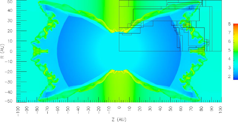
Figure 1: Density plot in units of $log_{10}(n_{proton}~{}cm^{-3})$ at time $t=7.1$ years. The black “hotboxes” delineate regions of enhanced refinement.

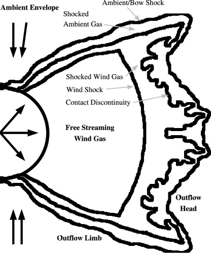
Figure 2: Flow region and discontinuity schematic.

The most important aspect of these simulations for the subject at hand is the fact that supersonic wind and ambient rotating molecular material are compressed at the wind and ambient shocks forming a thin layer around the contact discontinuity (figures 1 & 2). This layer then becomes a slip stream surface. The morphology of the outflow is also crucial and is the result of the ambient material’s density and velocity distributions (i.e. inertial and ram pressure confinement). Figures 3 & 4 show the kinematics of the flow with vectors indicating poloidal flow direction overlaid on a map of velocity magnitude (we defer discussion of rotation until the next section). Here one can see that wind material strikes the inner shock at an oblique angle. Post-shock wind is focused into a flow that streams parallel to the contact discontinuity. This high speed shocked wind moves ahead of the rest of the outflow, forming a cusp at mid to high latitudes that pushes past of the head of the outflow at the poles. These cusps are transient features and will eventually be subsumed into the rest of the outflow. Dense limbs of wind swept ambient material delineate the low latitude edges of the cavity. The dense limbs of the cavity and the narrow waist formed close to the inflow boundary are essential morphological signatures present in both our simulations and the source I maser spot observations.

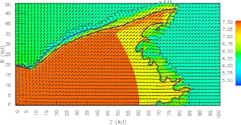
Figure 3: Magnitude of the total velocity of the flow field in units of $log10(cm~{}s^{-3})$ with arrows indicating flow direction. A plot that enhances the shear flow in the outflow limbs is shown in figure4. The inner line delineates the contact discontinuity. The outer line delineates the location of the cross cut in figure 8.

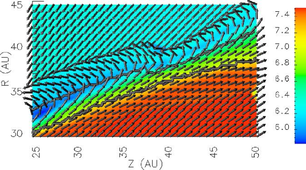
Figure 4: An enhancement of the shear region in the outflow limb shown in figure 3.

Velocity vectors of the flow pattern shown in figures 3 and 4 illuminate the formation of a slip stream between initially infalling ambient molecular material and outflowing wind material. The inner line in figure 3 delineates the contact discontinuity. This marks the transition between mostly wind material and mostly ambient material. Note that the change in direction of the velocity vectors as one moves from ambient to wind material. This flow reversal indicates the presence of a vortex across the interaction region. We identify the large density and velocity gradients present across the slip stream as susceptible to Kelvin-Helmholtz instabilities and will discuss these in more detail in the next section.

Thus to conclude this section we find our simulations show that a wind blown bubble with appropriate morphology for Source I will form via the interaction of a spherical wind with a collapsing, rotating envelope. In the next section we discuss both generic outflow issues raised by the simulations as well as specific connections to source I maser observations.

4 Discussion

We break our discussion into two sections. First we review our results in light of previous simulations of wind driven molecular outflows examining those features of the simulations which shed new light on unresolved issues. In the second section we compare our simulation results to the observations of Source I focusing particularly on the rotational patterns.

4.1 Generic Outflow Issues

Several authors (Shu, Ruden, Lada, & Lizano, 1991; Wilkin & Stahler, 1998; Lee, Stone, Ostriker, & Mundy, 2001) have constructed analytic models of the formation of bipolar molecular outflows. These models invoke the assumption that mixing between the shocked wind and shocked ambient gas occurs instantaneously. Such rapid and local mixing yields an outflow cavity that is delineated by a purely momentum driven thin shell and the swept up wind mass is taken to be negligible. The last assumption implies that the post-shock flow is dominated by shocked ambient gas. Thus gas will be carried along the shell downward toward the disk. Our simulation contradicts this model assumption. While there is much more mass in the ambient material, the momentum in the wind material is significant owing to the high velocity of the wind and the oblique nature of the wind shock. We find that the momentum of the wind material is dynamically important and must be incorporated into any model used to predict the kinematics inside the thin shell. This is true even in cases where turbulence dominates and the cavity walls are fully mixed. Delamarter, Frank, & Hartmann (2000) derive a condition for the mixed flow to be directed upward towards the head of the outflow:

$$\left[\frac{\dot{M}_{w}}{\dot{M}_{i}}\left(\frac{\tilde{M}_{sw}}{\tilde{M}_{si}}\right)^{2}\right]>1$$

where $\tilde{M}_{sw}$ is the Mach number of the shocked wind material and $\tilde{M}_{si}$ is the Mach number of the shocked infalling material.

For the parameters used in this simulation, $\dot{M}_{i}/\dot{M}_{w}=10$, $\tilde{M}_{sw}=5$, $\tilde{M}_{si}=.1$. Thus the left hand side of this equation evaluates to 250 and the condition for upward flow is satisfied. While the cavity walls in our simulations are not fully mixed we can compute the direction the flow would take if mixing occurred by averaging the momentum across the zones which comprise the shell. Figure 5 plots the effective velocity $v_{eff}$ that would result along the direction of the outflow cavity wall if the shocked layer were to become fully mixed. Here positive velocity indicates flow streaming upward towards the head of the cavity. Figure 5 shows the flow within the cavity walls to be positive at essentially all latitudes with a velocity of $v\sim 8~{}km~{}s^{-1}$. This result indicates that if the shocked flow were to mix by any means, the momentum of wind material would overwhelm that of the slower, denser ambient material resulting in poleward movement of material along the shell. Thus we conclude that the assumption that mixing within the bipolar outflow shell leads to a net downward streaming of mass towards the disk is incorrect.

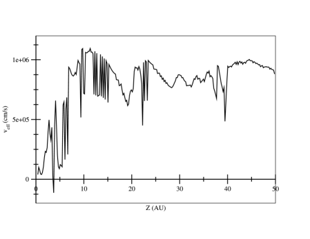
Figure 5: Net velocity of fully mixed shocked material along the direction of the contact discontinuity delineating the cavity wall.

Note that while do not see full mixing, our simulations do capture one net turnover in flow direction. We interpret the vortical reversal of vectors between the ambient shock and the wind shock as due to the development of Kelvin-Helmholtz instabilities and related mixing processes. This mixing results in the entrainment of outwardly directed wind momentum into the shocked ambient gas along the inner cavity walls. While our simulation clearly shows the vortical motions in the interaction region we operate with limited resolution due to computational constraints and cannot resolve the expected multiple non-linear Kelvin-Helmholtz roll-ups in this region. We rely, therefore, on an analytic description to quantify the unresolved instability responsible for entraining momentum from the wind into the region of ambient gas. The characteristic growth rate of the Kelvin-Helmholtz instability for wave mode $k$ is given by:

$$\Gamma_{kh}=|V_{sw}-V_{sa}|k\frac{\sqrt{\rho_{sw}\rho_{sa}}}{\rho_{sw}+\rho_{sa}}$$

where $\rho_{sw}$ and $V_{sw}$ denote the density and velocity on the shocked wind side of the slip stream and $\rho_{sa}$ and $V_{sa}$ denote the density and velocity on the shocked infalling side of the slip stream. We have computed the time scale for the growth Kelvin-Helmholtz modes $t_{kh}$ of wavelength $\lambda$, relative to the dynamical time scale of the outflow source as $1/\Gamma_{kh}=t_{kh}\approx 0.05t_{dyn}\lambda/r_{w}$ where $r_{w}$ is the distance from the central source to the wind shock. The analysis used here is for the Kelvin-Helmholtz growth across a thin shear layer. Since wavelengths less than the thickness of the slip stream layer are damped, we choose the wavelength of fastest growth equal to the width of the cavity wall or shell $\lambda\approx 0.25r_{w}$. Using values of the parameters taken from the simulations we find timescale for the growth of this mode is much less than the dynamical timescale of the outflow (i.e. $t_{kh}<<t_{dyn}=7.1~{}years$). This implies that unresolved Kelvin-Helmholtz instabilities will provide the mixing required to exchange momentum across the shear layer even though in our simulations we see a smooth (numerically) diffusive mixing in the shear layer. This result supports our interpretation that mixing has resulted in the entrainment of outwardly directed wind material into the layer of shocked ambient gas. With higher resolution we would expect to see the shear layer become more turbulent.

We now address the fragmentation of the head of the outflow in our simulations. While details of the polar caps of the outflow are not illuminated by the Source I $Si0$ maser observations, the fragmentation of the thin shell of swept-up ambient material in this region warrants some discussion. The presence of these fragments dominates the dynamics of the flow in the polar caps. We note that the dynamical age of the outflow in our model is very young; 7.1 years. A typical astrophysical outflow of much greater dynamical age would have time to produce even richer fragmentation and clumping spectrum than our the flow modelled in our simulation. The instability along the polar caps of the outflow and the formation of associated fragments and inhomogeneities is interesting in that it is characteristic of YSO molecular outflows (McCaughrean & Mac Low, 1997). The nature of “clumpy” flows remains largely unexplored though Poludnenko, Frank, & Blackman (2002); Meliolo et al. (2005) have examined properties of inhomogeneities on the propagation of shocks and the role such phenomena play in astrophysical contexts. Our simulations imply that such clumpy flows are likely to be a generic feature of bipolar outflows and jets.

We can, perhaps, understand the fragmentation seen in our simulations through known unstable modes of shocks. Vishniac (1983) has examined the stability of a thin spherical shock of wavelengths $>>$ than the thickness of the thin shell. They find that shocks that are sufficiently radiative to produce a density contrast of $\gtrsim 10$ are dynamically unstable. The growth rate associated with these modes are given by $\Gamma_{ts}\approx c_{s}/h$ where $c_{s}$ is the sound speed inside the thin shell and $h$ is the shell thickness. The characteristic temperature $10^{4}~{}K$ and shell thickness of $2~{}AU=0.1r_{w}$ along the thin dense shell at the rapidly expanding polar caps in the simulated outflow yield a timescale for the growth rate of this instability of $1/\Gamma_{ts}=t_{ts}\approx 0.04t_{dyn}$. Thus the rapid growth of the fragments which develop in this region are consistent with Vishniac’s analytic prediction.

4.2 Comparison with Observations

In this section we make a qualitative comparison between the broad morphological and kinematic properties of our simulations and those observed in the $SiO$ maser spots of Source I. We note that more detailed quantitative comparisons will require high resolution 3-D simulations including radiation-transfer calculations beyond the scope of the current work.

First we note our previous works have also shown that the opening angle of the outflow depends on the degree of flattening of the ambient material (Delamarter, Frank, & Hartmann (2000). Flatter, more pancake-like density (and infall velocity) distributions lead to more spherical bubbles with a larger opening angle for the arms of X. Thus the morphology of the models can be smoothly adjusted to fit the conditions in Source I. Most importantly the wide opening angle seen in the Source I masers argues strongly for the presence of a significant wide-angle wind component to the driving wind. While a jet component may still exist the laterial expansion of the lobes at the base would be difficult to reproduce without a wind component with significant momenta expanding into low latitudes.

We have proposed that the line of sight maser velocities observed about Source I are due to rotation. Specifically it is rotation retained by infalling molecular material that has been intercepted by a biconical outflow. We now demonstrate this assertion. Figures 6 & 7 show a color map of the rotational component of velocity $v_{\theta}$ in the shell of swept up material. The non-rotating wind material is delineated by the interior line. Notice that the region of greatest shear occurs midway between the outer edge of the ambient shock and the slip surface (CD). This is where the flow undergoes direction reversal across the slip stream. As discussed above we can identify this region as adjacent to the line of greatest vorticity generation. This region is most susceptible Kelvin-Helmholtz instabilities and the creation of related density inhomogeneities. The formation of fragments and filaments in this region would provide the density and path length enhancement most likely to result in the amplification of master spots. Because the masing material most likely lies in this region, its kinematics would be likely be revealed by observations of maser spots.

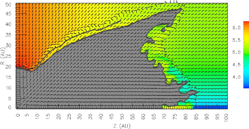
Figure 6: Magnitude of particle rotational velocity $v_{\theta}$ of the flow field in units of $log10(cm~{}s^{-1})$ with arrows indicating flow direction. The inner line delineates the contact discontinuity. The outer line delineates the location of the cross cut in figure 8.

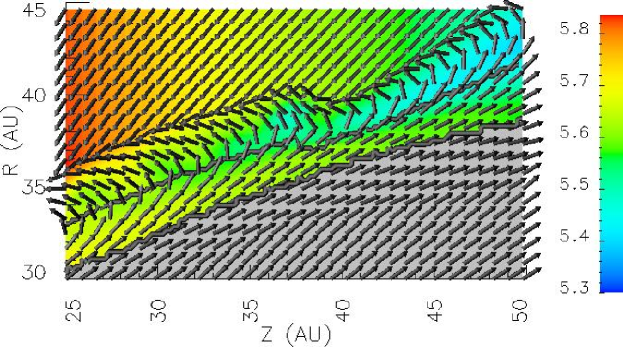
Figure 7: An enhancement of the shear region in the outflow limb shown in figure 6.

Figure 8 plots a cut of rotational velocity taken along this surface midway between the ambient shock and the contact surface. The magnitude of the rotational velocities is $3~{}km~{}s^{-1}<v_{rot}<15~{}km~{}s^{-1}$ in rough agreement with the line of sight velocities seen in the maser data. These values reflect the rotational velocities of the pre-shock ambient material. Thus as ambient material spirals inward towards the star it intercepts the cavity wall, is shocked and eventually reverses its poloidal but not its toroidal velocity. Our results thus indicate that the observed line of sight velocity of the maser spots can be interpreted as the rotation of infalling material that has been intercepted by a poorly collimated biconical outflow. Note that we correct for a systematic $\sim 5~{}km~{}s^{-1}$ redshift as is appropriate for the Orion region.

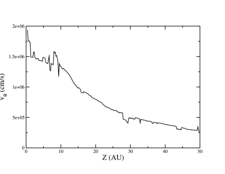
Figure 8: Rotational velocity vs distance along the z-axis taken along the surface midway between the position of highest density in the outer shell of shocked ambient material and the contact surface separating the wind launched and shocked ambient gases along the r-axis. The position of this cut is show in figures 3, 4 6 & 7.

Note also that our results show a decrease in rotational velocity as one moves outward along the arms of the X defined by the maser spots. The presence of a velocity gradient is ambigious in the observations. For example, in the data of Greenhill et al. (1998), the redshifted lobes show a velocity gradient with values ranging from $25~{}km~{}s^{-1}$ at the base of the X to $15~{}km~{}s^{-1}$ at its farthest extent. The blueshifted lobes do not show such a clear gradient however they do show a similar range of velocities. In our model gradients in $v_{rot}$ in the maser spots will reflect, to first order, gradients in the rotational velocities of the ambient material. A better accounting of turbulent advection of material along the walls of the cavity could smooth out the observed rotational gradient. However since no torques act on the swept up material conservation of angular momentum will still reduce its rotational velocity. Consideration of the initial conditions shows that the gradient in $v_{rot}$ is stronger in the radial direction than in height. Thus for models with wider opening angles the we expect the gradient to be less dramatic.

Finally one may ask if the rotation inferred for the Source I masers is due to the ambient material as we have modelled or if it comes from rotation of the stellar wind. We note that the observed maser proper motions of $\sim 15~{}km~{}s^{-1}$, which we take to be poloidal velocities along the shell, are an order of magnitude smaller than both typical young stellar object outflows and stellar winds. If this material were to originate from a disk wind it would have to emerge from a region quite far from the central source. Using $v_{escape}\sim v_{Keplerian}(R)$ gives $R\sim 40~{}AU$ which is quite far from the inner regions of the disk where launching is expected to be most effective (Ouyed et al., 2003). One might argue that the modest rotational gradient observed in the maser data indicates the presence of a magnetic field in the wind anchored to the disk such as would be the case for a disk wind. The field would then sustain the rotational motions of the wind material caught-up in the masers. However once any MHD launching mechanism takes a wind parcel out beyond the Alfvén radius the field will no longer provide rotational support for the wind and angular momentum conservation will reduce the wind’s rotational velocity as it expands. Since the Alfvén radius tends to be a few times larger then the radius of the footpoint of the flow, and the flow is likely to form close to the star at the inner regions of the disk, it is unlikely that the winds rotational motion can be magnetically supported. Thus the rotation seen in the masers are most convincingly interpreted as ambient material that has been swept up or entrained along shocks with the fast-moving wind (Greenhill et al., 2003; Doeleman, Lonsdale, & Pelkey, 1999). In all models, the $H_{2}$ densities and temperatures necessary for maser action, and the small line-of-sight velocity shifts necessary for maser amplification occurs along the limbs of the outflow.

5 Conclusion

Using AMR simulations we have explored the evolution of an outflow driven by a spherical wind from a massive gravitating source interacting with a rotating infalling cavity. The dynamics of the flow in the shocked ambient material are essential aspects of our model that have been neglected in previous works. Specifically, the growth of Kelvin-Helmholtz unstable modes in the slip stream between outflowing wind material and infalling molecular material along the cavity walls provides mixing at the wind/ambient gas interface. This mixing results in the outward acceleration and eventual direction reversal of initially infalling ambient material.

We have also shown that the head of the outflow will be unstable to thin shell instabilities. While this conclusion is not relevant to the observations of Source I it is of general interest for studies of molecular outflows. The fragmentation of radiatively cooling outflow lobes has important consequences for their long term dynamics and observational properties. The fact that our simulations show a rapid transition to fragmentation implies that molecular outflows on larger scales can be expected to be “clumpy” on a variety of scales. This issue should be addressed in future works.

We have compared our simulations with observations of maser spots in Source I in the BN/KL region in Orion. We find that when the wind evacuates a bipolar cavity, swept-up rotating ambient molecular material in the cavity walls is the likely source of the masers. This zone contains material which retains its rotation but which has been accelerated upward towards the head of the outflow lobe. The poloidal velocities seen in our simulations are of order those seen proper motions in the observations. The rotation retained by the shocked ambient material is consistent with the observed line of sight velocity of the maser spots observed about Source I. Thus we conclude that the line of sight motions in Source I inferred to be due to rotation (Greenhill et al., 2003, 2005) can be interpreted as originating in the rotation of the collapsing ambient material. Future work will need to explore the flow pattern in 3-D as well address issues related to formation of the masers in greater detail. We also conclude that the wide opening angle of the maser spot pattern is strong evidence that a significant wide angle wind component is at work in the Source I outflow.

Appendix A $H_{2}$ Microphysics

A.1 Cooling Functions

We employ a total cooling function $\Lambda=\Lambda_{LS}+\Lambda_{DM}+\Lambda_{OI}+\Lambda_{HeI_{D}}+\Lambda_{HI_{D}}+\Lambda_{H_{2\,D}}$. Where $\Lambda_{DM}=n_{H_{ion}}n_{e^{-}}\lambda_{DM}$ and $\lambda_{DM}$ is the atomic line cooling function appropriate for interstellar gases by Dalgarno & McCray (1972), the dominant cooling process at $T>10^{4}$. $\Lambda_{LS}$ is the $H_{2}$ cooling function of Lepp & Schull (1983) appropriate for a molecular gas. $\Lambda_{OI}=n_{HI}n_{OI}\lambda_{OI}(T)$ dominates the cooling at $T<300~{}K$ where $\lambda_{OI}(T)$ is the OI line cooling function tabulated by Launay & Roueff (1977). For temperatures greater than those listed in the table, $\lambda_{OI}(T)$ extrapolates with $\sqrt{T}$. Because the first ionization potential of $O$ is comparable to that of $H$, we use the abundance of molecular and atomic $H$ as a tracer for OI given as $n_{OI}=(n_{H_{2}}+n{HI})/n_{H_{ions}}f_{OI}$ where $f_{OI}=8.51\times 10^{-4}$ is the fractional coronal abundance of oxygen. The $\Lambda_{HeI_{D}}$, $\Lambda_{HI_{D}}$, and $\Lambda_{H_{2\,D}}$ terms account for cooling due to dissociation and ionization.

$$\Lambda_{HeI_{D}} = 24.60eVD_{HeI}$$

$$\Lambda_{HI_{D}} = 13.59eVD_{HI}$$

$$\Lambda_{H_{2\,D}} = 4.48eVD_{H2}$$

Where D represents the dissociation rates given in the following sections. Figure 9 shows each of these cooling rates for typical ISM density.

Figure 9: Cooling rates for typical ISM abundances, $n_{H_{2}}=2500$,$n_{HI}=5000$. $H_{2}$ is the molecular hydrogen cooling function, $H2-Dissociation$ is the thermal energy loss due to the dissociation of $H_{2}$ molecules, $OI$ is the singly ionized oxygen line cooling and $DM-atoms$ is the atomic line and recombination cooling function of Dalgarno & McCray.

A.2 Dissociation

Lepp & Schull (1983) fit an analytic function for the $H_{2}$ dissociation rate which takes the form:

$$\log_{10}(k^{H_{2},H}_{D})=\frac{\log_{10}k_{H}-\log_{10}(k_{H}/k_{L})}{1+n/n_{cr}}$$

where, for $H-H_{2}$ collisions, $\log_{10}(n_{cr})=4.00-0.416x-0.327x^{2}$ and, for $H_{2}-H_{2}$ collisions, $\log_{10}(n_{cr})=4.13-0.968x+0.119x^{2}$ with $x=\log_{10}(T/10^{4}K)$. $k_{H}$ and $k_{L}$ refer to the high ($n>>n_{cr}$) and low ($n<<n_{cr}$) density limits for the reaction rate. Lepp & Schull (1983) give:

$$k_{H}(T)=\left\{\begin{array}[]{ll}3.52\times 10^{-9}\exp(-4.39\times 10^{4}/T)\quad\textrm{for}\quad H-H_{2}\\ 5.48\times 10^{-9}\exp(-5.30\times 10^{4}/T)\quad\textrm{for}\quad H_{2}-H_{2}\\ \end{array}\right.$$

Lim et. al. (2002) Improve the dissociation low density dissociation rate of Lepp & Schull (1983) by using the more recent calculations for $k_{L}^{H-H_{2}}$ of Dove & Mandy (1986). Lim et. al. (2002) fit the results of Dove & Mandy (1986) to the form:

$$k_{L}(T)=4.69\times 10^{-14}T^{0.746}\exp(-5.55065\times 10^{4}/T)\quad\textrm{for}\quad H-H_{2}$$

We modify the original rates further by using the more recent calculations for low density $H_{2}-H_{2}$ dissociation of Martin et. al. (1998). We have also included corrections to the dissociation rate through the action of $He-H_{2}$ and $e^{-}-H_{2}$ collisions of Martin et. al. (1998) given by:

$$k^{i}_{D}(T)=\left(\frac{8dkT}{\pi\mu}\right)^{1/2}\frac{a(kT)^{b-1}\Gamma(b+1)\exp(-Eo/kT)}{\left(1+CkT\right)^{b+1}}\quad\textrm{for}\quad H_{2}-H_{2}$$

where $d=1.894\times 10^{-22}$ $k=3.167\times 10^{-6}$ and the constants a, b, c and Eo for each collision partner are given in table2 and $\mu$ is the reduced mass of the collision pair.

Table 2: Dissociation Rate Constants.

Partner	a	b	c	Eo
$H_{2}$	40.1008	4.6881	2.1347	0.1731
He	4.8152	1.8202	-0.9459	0.4146
$e^{-}$	11.2474	1.0948	2.1382	0.3237

The total dissociation rate is given by:

$$D_{H_{2}}=\sum_{i}n_{i}n_{H_{2}}k^{i}_{D}$$

where i ranges over all collision partners: $H_{2}$,$H$,$He$,and $e^{-}$.

A.3 Molecular Recombination Rate

Hollenbach & McKee (1979) give an approximation to the $H_{2}$ recombination rate due to HI “sticking” on dust surfaces as:

$$R_{H_{2}} = n_{H_{nuclei}}\,n_{HI}\,3\times 10^{-17}cm^{3}s^{-1}\frac{T_{2}^{1/2}f_{a}}{1+0.4(T_{2}+T_{dust\,2})^{1/2}+0.2T_{2}+0.08T_{2}^{2}}$$

$$T_{2} = T/100$$

$$f_{a} = 0.5=\textrm{ fraction of molecules that do not evaporate on dust surfaces.}$$

A.4 Shock Dissociation

As a test of these dissociation rates as implemented in our code we have computed the impulsively launched steady shock speed required for molecular dissociation. Figure 10 shows pre-shock density vs. shock speed for a steady shock resulting in 90% downstream $H_{2}$ dissociation. This result is consistent within a few $km~{}s^{-1}$ with the results of previous authors (Smith, 1994; Hollenbach & McKee, 1977).

Figure 10: Pres-hock density vs. shock speed for a steady shock resulting in 90% downstream $H_{2}$ dissociation.

A.5 Ionization & Recombination

Mazzotta et. al. (1998) catalog ionization and recombination rates for many species. We have employed HeI and HI ionization rates originally from Arnaud & Rothenflug (1985). Verner & Ferland (1996) fit the radiative recombination rate coefficients for several species including the He and H recombinations rates used for this work. We have included the fit to dielectric contribution to the He recombination rate of Mazzotta et. al. (1998).

References

- Arce (2003) Arce, H. G. 2003, Revista Mexicana de Astronomia y Astrofisica Conference Series, 15, 123
- Arnaud & Rothenflug (1985) Arnaud, M. & Rothenflug, R. 1985, A&AS, 60, 425
- Barvainis (1984) Barvainis, R. 1984, ApJ, 279, 358
- Balsara (1999) Balsara, Dinshaw S. 1999, J. Comput. Phys., 148, 133
- Bragg et. al. (1982) Bragg, S. L., Smith, W. H., & Brault, J. W. 1982, ApJ, 263, 999
- Chandler & Greenhill (2002) Chandler, C. J., & Greenhill, L. J. 2002, Astronomical Society of the Pacific Conference Series, 267, 357
- Chernin & Wright (1996) Chernin, L. M. & Wright, M. C. H. 1996, ApJ, 467, 676
- Dalgarno & McCray (1972) Dalgarno, A. & McCray, R. A. 1972, ARA&A, 10, 375
- Delamarter, Frank, & Hartmann (2000) Delamarter, G., Frank, A., & Hartmann, L. 2000, ApJ, 530, 923
- Doeleman, Lonsdale, & Pelkey (1999) Doeleman, S. S., Lonsdale, C. J., & Pelkey, S. 1999, ApJ, 510, L55
- Dove & Mandy (1986) Dove, J. E. & Mandy, M. E. 1986, ApJ, 311, L93
- Frank (1999) Frank, A. 1999, New Astronomy Review, 43, 31
- Frank & Mellema (1996) Frank, A. & Mellema, G. 1996, ApJ, 472, 684
- Gardiner, Frank, & Hartmann (2003) Gardiner, T. A., Frank, A., & Hartmann, L. 2003, ApJ, 582, 269
- Genzel & Stutzki (1989) Genzel, R. & Stutzki, J. 1989, ARA&A, 27, 41
- Gezari (1992) Gezari, D. Y. 1992, ApJ, 396, L43
- Greenhill et al. (1998) Greenhill, L. J., Gwinn, C. R., Schwartz, C., Moran, J. M., & Diamond, P. J. 1998, Nature, 396, 650
- Greenhill et al. (2003) Greenhill, L.J., Reid, M.J., Diamond, P.J., Elitzur, M. 2003, IAU Symp. 221, Star Formation at High Angular Resolution, eds. Burton et al., ASP, (astro-ph/0309334)
- Greenhill et al. (2005) Greenhill, L.J., Reid, M.J., Diamond, P.J., Elitzur, M. 2005, ApJ, submitted
- Hartmann, Calvet, & Boss (1996) Hartmann, L., Calvet, N., & Boss, A. 1996, ApJ, 464, 387
- Hollenbach & McKee (1979) Hollenbach, D. & McKee, C. F. 1979, ApJS, 41, 555
- Hollenbach & McKee (1977) Hollenbach, D. & McKee, C. F. 1980, ApJ, 241, L47
- Icke (1988) Icke, V. 1988, A&A, 202, 177
- Königl (1999) Königl, A. 1999, New Astronomy Review, 43, 67
- Konigl & Pudritz (2000) Konigl, A., & Pudritz, R. E. 2000, Protostars and Planets IV, 759
- Lane (1982) Lane, A. P. 1982, Ph.D. Thesis,
- Launay & Roueff (1977) Launay, J. M. & Roueff, E. 1977, A&A, 56, 289
- Lee, Stone, Ostriker, & Mundy (2001) Lee, C., Stone, J. M., Ostriker, E. C., & Mundy, L. G. 2001, ApJ, 557, 429
- Lepp & Schull (1983) Lepp, S. & Shull, J. M. 1983, ApJ, 270, 578
- Leveque (1997) Leveque, Randall J. 1997, J. Comput. Phys., 331, 327
- Lim et. al. (2002) Lim, A. J., Raga, A. C., Rawlings, J. M. C., & Williams, D. A. 2002, MNRAS, 335, 817
- Mandy & Martin (1993) Mandy, M. E. & Martin, P. G. 1993, ApJS, 86, 199
- Martin et. al. (1998) Martin, P. G., Keogh, W. J., & Mandy, M. E. 1998, ApJ, 499, 793
- Mazzotta et. al. (1998) Mazzotta, P., Mazzitelli, G., Colafrancesco, S., & Vittorio, N. 1998, A&AS, 133, 403
- Mellema, Eulderink, & Icke (1991) Mellema, G., Eulderink, F., & Icke, V. 1991, A&A, 252, 718
- Meliolo et al. (2005) Melioli, C., Dal Pino, E., & Raga, A., 2005, A&A, in press
- Menten & Reid (1995) Menten, K. M. & Reid, M. J. 1995, ApJ, 445, L157
- McCaughrean & Mac Low (1997) McCaughrean, M. J. & Mac Low, M. 1997, AJ, 113, 391
- Ouyed et al. (2003) Ouyed, R., Clarke, D. A., & Pudritz, R. E. 2003, ApJ, 582, 292
- Plambeck, Wright, & Carlstrom (1990) Plambeck, R. L., Wright, M. C. H., & Carlstrom, J. E. 1990, ApJ, 348, L65
- Plewa & Müller (1999) Plewa, T. & Müller, E. 1999, A&A, 342, 179
- Poludnenko, Frank, & Blackman (2002) Poludnenko, A. Y., Frank, A., & Blackman, E. G. 2002, ApJ, 576, 832
- Poludnenko et. al. (2004) Poludnenko, A., Varniere, P., Frank, A., & Mitran S, 2004, to appear in Springer’s Lecture Notes in Computational Sciences and Engineering (LNCSE) series
- Quillen et al. (2004) Quillen, A., Frank, A., Cunningham, A., Blackman, E., & Pipher, J., 2004, ApJ, submitted
- Richer et al. (2000) Richer, J. S., Shepherd, D. S., Cabrit, S., Bachiller, R., & Churchwell, E. 2000, Protostars and Planets IV, 867
- Shu, Ruden, Lada, & Lizano (1991) Shu, F. H., Ruden, S. P., Lada, C. J., & Lizano, S. 1991, ApJ, 370, L31
- Shu et al. (2000) Shu, F. H., Najita, J. R., Shang, H., & Li, Z.-Y. 2000, Protostars and Planets IV, 789
- Shepherd (2003) Shepherd, D. 2003, Astronomical Society of the Pacific Conference Series, 287, 333
- Smith (1994) Smith, M. D. 1994, MNRAS, 266, 238
- Snyder & Buhl (1974) Snyder, L. E. & Buhl, D. 1974, ApJ, 189, L31
- Ulrich (1976) Ulrich, R. K. 1976, ApJ, 210, 377
- Varnie et. al. (2004) Varniere, P., Poludnenko, A., Cunningham, A., Frank, A., & Mitran S, 2004, to appear in Springer’s Lecture Notes in Computational Sciences and Engineering (LNCSE) series
- Verner & Ferland (1996) Verner, D. A. & Ferland, G. J. 1996, ApJS, 103, 467
- Vishniac (1983) Vishniac, E. T. 1983, ApJ, 274, 152
- Wilkin & Stahler (1998) Wilkin, F. P. & Stahler, S. W. 1998, ApJ, 502, 661
- Woitas et al. (2005) Woitas, J., Bacciotti, F., Ray, T. P., Marconi, A., Coffey, D., & Eislöffel, J. 2005, A&A, 432, 149
- Wright & Plambeck (1983) Wright, M. C. H. & Plambeck, R. L. 1983, ApJ, 267, L115
- Wright, Plambeck, & Wilner (1996) Wright, M. C. H., Plambeck, R. L., & Wilner, D. J. 1996, ApJ, 469, 216