Rotational Widths for Use in the Tully-Fisher Relation. I. Long-slit Spectroscopic Data

Abstract

We present new long-slit $\rm H\alpha$ spectroscopy for 403 non-interacting spiral galaxies, obtained at the Palomar Observatory 5 m Hale telescope, which is used to derive well-sampled optical rotation curves. Because many of the galaxies show optical emission features which are significantly extended along the spectrograph slit, a technique was devised to separate and subtract the night sky lines from the galaxy emission. We exploit a functional fit to the rotation curve to identify its center of symmetry; this method minimizes the asymmetry in the final, folded rotation curve. We derive rotational widths using both velocity histograms and the Polyex model fit. The final rotational width is measured at a radius containing 83% of the total light as derived from I-band images. In addition to presenting the new data, we use a large sample of 742 galaxies for which both optical long-slit and radio HI line spectroscopy are available to investigate the relation between the HI content of the disks and the extent of their rotation curves. Our results show that the correlation between those quantities, which is well-established in the case of HI-poor galaxies in clusters, is present also in HI-normal objects: for a given optical size, star formation can be traced further out in the disks of galaxies with larger HI mass.

1. Introduction

Accurately determined rotational velocities of spiral galaxies are important tools of extragalactic astronomy and cosmology. Among other applications, they serve to derive masses and redshift-independent distances of galaxies, to characterize the peculiar velocity field in the local universe, to probe the impact of tidal and collisional forces and to derive mass-to-light ratios and their evolution. Of particular note, the accuracy of the rotational velocity measurement is the single dominant contributor to the error budget of the Tully-Fisher (TF; Tully & Fisher, 1977) relation, beyond the intrinsic scatter (Giovanelli et al., 1997b). The full characterization of a galaxy’s velocity field ideally requires a two-dimensional map, such as can be obtained by means of HI synthesis, Fabry-Perot or fiber bundles. Such maps can provide direct evidence for departures in the velocity field from circular rotation and planarity and can best allow the extraction of the contribution of circular rotation. However, those techniques have become available relatively recently, and they are still observationally costly (Fabry-Perot systems do not allow for simultaneous sampling of the velocity channels) or characterized by limited spatial dynamic range (fiber bundles). For these reasons, the vast majority of velocity width data have relied on simpler, albeit cruder, observations, e.g. one-dimensional rotation curves (RC) $V(r)$ obtained with single-slit spectrographs placed along a spiral disk’s major axis or, even more commonly, with the zero-th order approach of 21cm global (i.e., spatially integrated) line profiles obtained with single radio dishes. In practical situations such as wide area peculiar velocity studies exploiting the TF relation, it is often necessary to combine rotational velocity measures obtained from multiple methods. In such cases, it is imperative to devise width measurement algorithms that are both robust and minimize technique-based bias or systematic effects. This paper is the first of a series in which we use a large compilation of both global HI line profiles and optical long-slit spectra to minimize such systematics for TF applications and to derive a statistical characterization of how disks rotate.

Most optical studies of rotation velocities in the low redshift universe concentrate on the red part of the optical spectrum, made attractive by the presence of several nebular lines, most prominently $\rm H\alpha$ at 6563Å and [NII]$\lambda\lambda$6548,6584Å. The radial variation of the observed rotational velocities – the rotation curve – offers insight into the velocity field but must be interpreted in light of assumptions about dark matter components, spatial and kinematic disturbances and asymmetries, the impact of extinction, and likely biases induced by differences in the global star formation history. Several recent works have contributed significant compilations of velocity widths based on optical long-slit spectra, including Mathewson et al. (1992), Mathewson & Ford (1996), Courteau (1997, hereafter C97), Vogt (1995), Vogt et al. (2004a), Dale (1998), and Dale et al. (1997, 1998, 1999a,b,c, 2001). Rotational widths presented by those authors have been derived using several different algorithms, based either on velocity histograms (Mathewson, Vogt, and their collaborators) or on functional fits to the RCs (C97; Dale and collaborators). The current work presents new data and widths based on a measurement technique belonging to the second category. Discussion of the systematics using a large compilation including all of the above referenced datasets but with rotational widths remeasured on the digital spectra according to the technique presented here will be presented separately (Catinella et al., 2005b, hereafter Paper II).

The principal issue is: given a RC, what specific measurement of a characteristic velocity width best reflects a physical quantity tied to the galaxy’s rotational velocity. The circular velocity field of a galaxy can be calculated from the expression describing the gravitational potential of the system, under the assumption of centrifugal equilibrium. In the case of an infinitely thin disk, characterized by an exponential surface density distribution with scale length $r_{\rm d}$, it can be shown (Freeman, 1970) that the resulting RC reaches a peak at 2.12 $r_{\rm d}$, and approaches the asymptotic Keplerian law at larger galactocentric distances. In this simple case, one could identify the velocity width with the value of the maximum rotation of the disk (or twice its value). The observational discovery that most RCs are not falling, but rather flat or even rising at the edge of the optical disk, raised the issue of accounting for matter that was not detectable except for its gravitational effects. The circular velocity field should be thus calculated from the sum in quadrature of two terms, related to the exponential disk and the dark matter halo; the effect of a stellar bulge can be included similarly.

For simplicity, the “dark” halo is usually assumed to be spherical. Two common choices for the expression of its radial density distribution are the so-called isothermal and NFW (Navarro et al., 1997) profiles, the latter derived from N-body simulations of structure formation in hierarchically clustering universes. The observed RCs, or at least their large-scale, smooth behavior (neglecting spiral streaming, bar perturbations, disk warps or asymmetries, and so on), can be successfully modeled using these components, and giving them appropriate weights in order to optimize the results. The presence of a dark matter halo complicates however the definition of rotational width, since it should no longer be associated with the peak of the RC, but the appropriate radial distance at which a characteristic width measurement should be made is not obvious. While several authors measure rotational velocities at 2.15 $r_{\rm d}$ (e.g., Chiba & Yoshi 1995 and C97), others prefer to do it at the optical radius $R_{\rm opt}$, i.e., the radius encompassing 83$\%$ of the total integrated light of the galaxy (e.g., Persic et al. 1996; Giovanelli et al. 1997a. For comparison, $R_{\rm opt}$=3.2 $r_{\rm d}$ for an exponential disk). The sampling of the velocity fields at larger galactocentric distances offers important advantages in terms of smaller extinction and shallower (if not null) velocity gradient, since both dust fraction and RC slope decrease with increasing radius. For these and other reasons, further discussed here and in Paper II, we adopt $R_{\rm opt}$ as reference radius for width measurements. Our approach to determining rotational velocities from long-slit RCs is described in detail in this work. Rotational velocities obtained from optical long-slit spectra should, however, be compared to radio widths derived from HI integrated line profiles, using large samples of galaxies with both measurements available. This is a key element to address the issue of a reference scale for RC width measurements. Since HI emission can be traced out to radial distances that are typically twice as large as those sampled by HII regions, HI widths should provide, in fact, more reliable estimates of the maximum rotation of the disks. Such comparison will be presented in Paper II.

This paper is organized as follows: We describe our sample selection criteria, observation strategy, and data reduction process in Section 2. The RC extraction and folding technique are discussed in Sections 3 and 4. We illustrate our velocity width measurement method in Section 5, and present our results in Section 6. The relation between the distributions of the $\rm H\alpha$ and HI line emissions in the disks, which is relevant to the determination of velocity widths, is investigated for a large overlap sample with both radio and optical spectroscopy in Section 7, and our conclusions are summarized in Section 8.

2. Observations and Data Reduction

The optical long-slit spectroscopy presented in this work was obtained at the Palomar Observatory 5 m Hale telescope. A total of 20 nights (19 of which had weather conditions adequate for spectroscopy) were allocated over the course of five observing runs. To minimize overheads and maximize throughput, spectra were obtained using only the red camera of the Double Spectrograph (Oke & Gunn, 1982) at the Cassegrain focus (f/15.7). The combination of the 1200 lines mm^-1 grating and a 2″ wide slit yielded a dispersion of 0.65 Å pixel^-1; the spatial scale of the CCD was 0.468″ pixel^-1. The grating angle was set in order to obtain a spectral coverage of 6530-7180 Å, allowing detection of the $\rm H\alpha$ line up to $cz\simeq$ 28,000 km s^-1. In addition, a small number of spectra were acquired with similar instrumental setup during other observing runs by members of our group. A few galaxies have been observed more than once to check the consistency among different runs. Of the 532 galaxies targeted, 488 show $\rm H\alpha$ emission (12 of the remaining ones show $\rm H\alpha$ in absorption; the other 32 have continuum but no line emission within the observed wavelength range). The final number of galaxies with useful, extended RCs is 403.

The sample targeted for the long-slit observations was extracted from a larger set of spirals identified as good TF candidates for inclusion in a photometric I-band survey carried out by M.P.H., R.G., and collaborators as a part of an effort to map the peculiar velocity field in the local Universe. Several datasets containing I-band photometry, optical RCs derived from long-slit spectra, and global HI profiles all in digital format contribute to what will be referred to as the SFI++ sample; details of this compilation will be discussed more fully elsewhere (Catinella 2005; Masters et al., in preparation). The spectroscopic sample presented here includes undisturbed, inclined spirals with apparent diameter greater than 0.6′, as estimated from a quick-look examination of the I-band images. The targets were identified principally to provide adequate TF target sampling in the sky area just south of the celestial equator, $-15^{\circ}\leq\delta\leq 0^{\circ}$, and to provide optical rotation widths for objects for which HI global profiles were not available for one of various reasons. The resulting sample for the $\rm H\alpha$ spectroscopy was heterogeneous, and included three types of targets: (a) galaxies with no spectroscopy (optical or radio) available; (b) galaxies with problematic HI profiles (due to confusion within the radiotelescope beam, or with irregular, asymmetric profiles, where a velocity width could not be clearly determined), and (c) a minority of nearby galaxies with apparent sizes larger than the spectrograph slit, where observations obtained at multiple offset positions along the major axis were required to trace the full extent of the velocity field. A few additional targets (14 galaxies) for which I-band photometry was not available were observed to fill in gaps in our observing schedule.

Due to the heterogeneous composition of the observational sample, we adopted a slightly different observing strategy depending on the category (a, b, or c in the previous paragraph) to which each target belonged. In the absence of previously available spectroscopic information (the majority of the cases), we performed a first, 5 minute integration on the target. A quick inspection of the spectrum allowed us to check for the presence of extended galaxy line emission, and to estimate the strength of the spectral lines. If the observation was deemed useful for TF purposes, a second integration long enough to adequately sample the outer disk regions (typically 10-15 minutes) was performed. For some other targets, prior information on the strength of HI line emission suggested that $\rm H\alpha$ would be detectable; in such cases, we performed a 10 minute integration. Finally, in those cases where the 128″-long slit did not sample the full extent of the RC, we acquired one or more “offset” spectra, displaced by multiples of 45″ from the central position, along the major axis of the galaxy. This technique was particularly designed to insure that the outer parts of large objects are adequately sampled.

The spectra have been reduced using standard and customized IRAF tasks. The standard reduction procedure includes the following steps: bias subtraction, flat-fielding, cosmic ray cleaning, line-curvature correction (modeled from the night sky emission lines; the “S-distortion” was found not to be significant and thus ignored), and wavelength calibration (using the sky lines). Multiple exposures of the same galaxy at the same slit position were co-added, sky lines and galactic continuum were fit with polynomials and then subtracted from the spectra. In the remainder of this section, we will discuss the sky subtraction in detail, focusing on the case of galaxies with line emission significantly extended relative to the size of the slit.

2.1. A New Technique for Sky Line Subtraction

The standard sky subtraction technique requires the identification of signal-free regions on both sides of the galaxy line emission, along the spatial direction; for each spectral channel, the sky lines in those narrow strips are then interpolated with a low-order (2 or 3, typically) polynomial, and subtracted from the spectrum. Such a procedure is clearly not applicable if the galaxy line emission fills the spectrograph slit. In particular, this problem affects 73 galaxies in our sample which are sufficiently extended to require offset observations. We thus developed a modification of the standard technique to deal with this issue.

We illustrate our technique (which will be referred to as template sky subtraction) using the galaxy MCG-2-31-017 (AGC 520006) as an example. MCG-2-31-017 is an Scd spiral, characterized by weak continuum and strong line emission; its heliocentric velocity is 4460 km s^-1. Figure 1a shows the portion of its spectrum that includes the galaxy emission lines (before continuum and sky subtraction). The horizontal and vertical axes correspond to spatial position along the slit and dispersion, respectively. The $\rm H\alpha$ line is the most prominent feature in the lower half of the spectrum. The lack of signal-free regions at the edges of the slit leads to a very poor sky line subtraction, when the standard procedure is applied (Figure 1c; the galaxy continuum emission has also been removed). The use of a few pixels on both sides of each row of Figure 1a cannot, in fact, constrain the shape of the sky and continuum emission, except at the very edges of the slit, and thus the sky subtraction leaves large residuals across the spectrum (horizontal chop in Figure 1c). The result for the sky line-free region would significantly improve if the continuum emission was removed first (i.e., if the sky subtraction was applied to Figure 1b instead of 1a), but the residuals in the region of interest for RC extraction would be unchanged. This result can be greatly improved by subtracting a sky line template spectrum, specifically constructed for MCG-2-31-017, from the continuum-free spectrum shown in Figure 1b. The sky template is a spectrum that contains only sky lines, with positions and intensities that match those in Figure 1b as closely as possible, at least near the $\rm H\alpha$ line. It is obtained by taking the median of the continuum-subtracted spectra of three or more reference galaxies, showing no line emission in the redshift region where the $\rm H\alpha$ line of the target galaxy lies. Each reference spectrum must be precisely aligned with the target spectrum to match the positions of its sky lines (with an accuracy of a few tenths of a pixel). Finally, the intensities of the template sky lines are optimized for the target spectrum by multiplying the template by a small numeric factor. Such factor is chosen upon examination of the residuals of the template subtraction near the $\rm H\alpha$ line. If the residuals are positive for some sky lines and negative for others, the scaling factor used is that providing the most reliable RC (in this sense, a sky line residual running across the brightest part of the $\rm H\alpha$ line does not affect the RC, whereas one that overlaps with the low signal-to-noise parts does). The identification of suitable reference galaxies can be very challenging, because not only the intensity of each sky line changes (depending on integration time and atmospheric conditions), but also the relative intensity of different sky lines can vary significantly over the course of the same night. More details on the choice of reference spectra can be found in Catinella (2005). The result of the template subtraction for MCG-2-31-017 is shown in Figure 1d: our method has substantially improved the quality of the sky subtraction. Figures 2a and 2b show the RCs extracted from the spectra in Figures 1c and 1d, respectively. The dotted lines indicate the center of symmetry of the RC, identified by the average of the 90th and 10th percentile velocities (kinematic center, discussed in § 4). The error bars are obtained from Gaussian fits to the $\rm H\alpha$ line profile at each spatial position, as explained in § 3. A close inspection of Figure 2 shows that the RC in (b) is less noisy and traces slightly farther out than that in (a). The number of data points (112 and 104, respectively) affects the values of the percentile velocities used to identify the kinematic center, and accounts for the small offset (6 km s^-1) between the central velocities in the two cases.

In general, different templates are required for different objects, nights, or even different emission lines of the same galaxy, making this sky subtraction technique very time-consuming (unless the sky lines are fairly stable over a given night, in which case the same template might be used for multiple target spectra). Whether the result is worth the effort involved depends on the purpose of the observation and on the characteristics of the emission of the galaxy considered. In fact, the standard and template sky subtraction provide essentially the same RC width for MCG-2-31-017, but for galaxies with fainter $\rm H\alpha$ emission, or for purpose of studying the details of the RC in its outer parts especially, this template fitting technique can produce a more robust measurement than the standard approach.

It is interesting to mention another approach to a similar sky-subtraction issue, developed by Bershady et al. (2005, hereafter B05) for integral-field fiber spectroscopy. The subtraction of night sky emission for multifiber data has been a long-standing problem, usually dealt with by adopting observing techniques in which the telescope is nodded between targets and adjacent sky positions. This strategy is successful but not very efficient, since only half of the observing time is spent on the targets. An alternative solution based on a different sky subtraction algorithm has been recently proposed and tested on spectra obtained with SparsePak, a formatted fiber array optimized for spectroscopy of low surface brightness galaxies, described in Bershady et al. (2004). Following the approach explained in detail in B05, the wavelength-calibrated and rectified multifiber spectra obtained from each observation are arranged into a two-dimensional image format, sorted by position along the slit (with the interfiber gaps taken out). The result is analogous to, and processed as, a long-slit spectrum. As Figure 14 of B05 shows, the problem is similar to that discussed in this section: the source line emission spans the whole extent of the slit, making the subtraction of the sky lines very difficult. In the case of the SparsePak observations, 7 of the 82 fibers were assigned to sky. Sky subtraction schemes that rely on a very small number of sky pixels, however, yield noisy results, similar to those shown in Figure 2c for our dataset. A significant improvement is obtained by using all the spatial channels (fibers): the spectrum is continuum-subtracted first (as we do for our spectra before template subtraction), and a low-order polynomial is then fit to each spectral channel, with a clipping algorithm that rejects spatial channels with source flux. This algorithm can be applied to continuum-subtracted long-slit spectra, provided that (a) there are enough source-line-free pixels at each wavelength to constrain the fit to the sky line profile, and (b) the shape of the sky line profiles is symmetric with respect to the center of the slit (so that the sky line fit over half slit fairly matches the other half). The second condition is certainly met by our Palomar spectra. In fact, for galaxies with line emission spilling over one side only of the slit, we removed the sky lines by fitting a first-order polynomial using only the signal-free side of the spectrum (if there were enough pixels to do so). When this method is applicable, it produces final spectra that are generally cleaner than those obtained via template subtraction.

In conclusion, both B05 and our template approaches can provide a significantly improved sky subtraction for long-slit spectra where the galaxy emission fills the slit. Which method should be used depends on the characteristics of the source emission – whereas B05’s algorithm avoids all the complications associated with the construction of a sky template (the choice of suitable reference galaxies, image registration, and intensity rescaling), its application requires a large enough number of signal-free pixels at each wavelength to constrain the sky line fits.

3. Rotation Curve Extraction

Once continuum and sky line subtracted, the spectra are ready for RC extraction. Since the typical seeing at the Palomar Observatory is $\sim$1″-2″, and the CCD spatial scale used was $\sim$0.5″ pixel^-1, the RCs are clearly oversampled. Therefore, we Hanning smoothed the spectra and recorded the peak value of the velocity (from a Gaussian fit across the $\rm H\alpha$ line) for every other pixel. The errors on the peak velocities were obtained through a Monte-Carlo resampling technique (an algorithm used by non-linear fitting tasks in IRAF to estimate coefficient errors): each section across the spatial axis of the Hanning-smoothed spectrum was replicated 15 times, each point being replaced by its value from the Gaussian fit plus noise with dispersion given by the RMS of the fit. A Gaussian fit was performed for each replication, and the dispersion of the fitted peak values used to estimate the velocity errors. All the points of the extracted RC were individually inspected, with particular attention to those belonging to low signal-to-noise regions, and only those with reliable Gaussian fits were kept. The profile of the $\rm H\alpha$ line at each spatial position is usually well approximated by a Gaussian, with the possible exception of the innermost parts of the galaxies, where non-circular motions sometimes cause secondary peaks and deviations from the Gaussian shape (however such regions are typically those with the strongest $\rm H\alpha$ emission, and therefore the positions of the profile peaks are well determined).

RCs with strong continuum emission or central bars, which mostly arise in earlier type (Sa-Sb) spirals, often show $\rm H\alpha$ absorption in the nuclear regions, due to the strong Balmer absorption features of A-type stars. In these cases, we used another emission line, typically [NII]$\lambda 6584$ Å  if available, to fill in the central gaps of the $\rm H\alpha$ RC. The [NII]$\lambda 6584$ Å and $\rm H\alpha$ RCs were extracted separately, matched, and the [NII]$\lambda 6584$ Å data points kept only if lying within $\rm H\alpha$ gaps. We applied a [NII]$\lambda 6584$ Å patch to approximately 15$\%$ of our $\rm H\alpha$ RCs.

When offset observations of the same galaxy (at the same slit position angle) were available, the RCs separately extracted from each spectrum were combined by matching their common features. In the region where the RCs overlap, we did not average the data points, but rather keep the ones with higher signal-to-noise ratio. As an aside, we point out that since offset observations farther from the galaxy center were typically integrated for a longer time, a stronger feature (i.e., smaller error bars) in the combined RC does not necessarily represent a stronger intensity of the underlying HII regions.

4. Rotation Curve Folding

In order both to measure the velocity width using our algorithm (see § 5) and to determine the systemic recessional velocity, the rotation curves must be folded about a central origin, typically chosen as either the photometric center-of-light, or the kinematic center. The definition of the latter itself varies; one common method identifies the folding center with the velocity closest to the average of $V_{10}$ and $V_{90}$, the 10th and 90th percentile points of the RC velocity histogram (notice that since there are no spatial interpolations involved, the two sides of the folded RC are sampled on the same spatial grid). As shown by Dale et al. (1997), kinematic centering appears preferable in most cases, because it avoids misidentification of the photometric center due to bars or extinction within the galaxy. Moreover, the estimate of the light peak position is very poor in galaxies with a weak or nearly absent continuum emission (16$\%$ of our sample), and in galaxies with nuclear regions dominated by $\rm H\alpha$ absorption (15$\%$ of our sample). On the other hand, if a RC is significantly asymmetric or unevenly sampled (as in the case of galaxies that required offset observations), the kinematic centering will also provide an unsatisfactory folding. This is shown in Figure 3a for MCG-3-05-008 (AGC 410269), a galaxy with a rising RC, where the $\rm H\alpha$ emission is traced farther out in one of the arms.

A better result can be obtained making use of the detailed shape of the RC by fitting an anti-symmetric function to the unfolded RC and leaving the spatial position and velocity of the center as free parameters. For its convenience and in order to minimize the number of fitting parameters, we adopt the Universal Rotation Curve (URC) description proposed by Persic et al. (1996) which incorporates contributions both from a stellar exponential thin disk and a spherical dark matter halo. Although inadequate to model individual RCs as already pointed out elsewhere (e.g., C97; Willick, 1999), the URC provides a useful parameterization of the average RC of a galaxy in terms of its luminosity and optical radius $R_{\rm opt}$. In particular, the URC description approximates the overall shape of a RC adequately for the purpose of determining its center of symmetry.

In order to apply the URC folding method, we make use of the detailed SFI++ I-band photometric data available to us, assigning to each galaxy its corresponding URC model based on its I-band luminosity, $R_{\rm opt}$, and inclination, and leave a scale factor and a small offset from the kinematic center, in both radial and velocity directions, as free parameters determined via a non-linear least square fit to the RC data points. Figure 3b demonstrates that this technique (URC folding) is remarkably more successful than the simple kinematic one based on the histogram method, shown in (a), at folding asymmetric RCs. As expected, for symmetric RCs the two folding methods give essentially the same result. As discussed in § 5, we measure the rotational velocity of a disk galaxy at $R_{\rm opt}$ from a functional fit (Polyex model, also shown in Figure 3b) to its folded RC. It should be noted that the RC folding is not strictly necessary for this type of width measurement, but the identification of the RC center cannot be avoided. In fact, other authors prefer to add two parameters to the expression used to model a RC, solving for its shape and center at the same time (e.g., C97).

In order to assess the comparative validity of the kinematic and URC folding techniques on a quantitative basis, we make use of the larger SFI++ sample and test their respective ability to minimize the asymmetry of the folded RCs. As a measure of asymmetry, we adopt the definition given by Dale & Uson (2003):

$${\rm Asymmetry}=\sum\frac{||V(R)|-|V(-R)||}{\sqrt{\sigma^{2}(R)+\sigma^{2}(-R)}}$$

$$\times\left[\frac{1}{2}\sum\frac{|V(R)|+|V(-R)|}{\sqrt{\sigma^{2}(R)+\sigma^{2}(-R)}}\right]^{-1}$$ (1)

where $V(R)$ and $\sigma(R)$ are velocity and corresponding uncertainty at the radial position $R$, and the summation symbols refer to radial distances for which both arms are sampled (unpaired RC data points are excluded). The quantity defined in Equation 1 simply measures the area between the two folded RC arms, normalized by the average area that they subtend. The calculation of the asymmetry index is slightly more complicated for the URC-folded RCs, because in general the two arms are not sampled on the same spatial grid (due to a small spatial offset from the kinematic center). We therefore calculate two indices for each RC by pairing the points on one arm with those obtained by interpolation of the other arm at the same spatial positions, and take their average as our measure of asymmetry.

The distributions of the URC and kinematic asymmetry indices of the 999 optical RCs with available velocity error information in our digital archive are presented in Figure 4. The histogram obtained for the URC folding (solid) is more centrally concentrated than the one corresponding to kinematic folding (hatched), indicating that the first technique is more effective at minimizing the overall asymmetry of the RCs. The mean asymmetry indices for the URC and kinematic cases are 11.3$\pm$0.3% and 19.4$\pm$0.5%, respectively; for comparison, Dale et al. (2001, hereafter D01) obtained an average asymmetry of 12.5$\pm$1.0% applying Equation 1 to a sample of field galaxies (in the foreground or background of clusters) with RCs folded according to the kinematic histogram technique. Both D01 and our samples were selected for TF studies, have similar morphological composition (dominated by normal late-type spirals, mostly Sc), and were obtained with similar instrument setup (most of the D01 spectroscopy was carried out with the Palomar 5m telescope); however the characteristic redshift of our galaxies is smaller (typically $z\lesssim 0.03$, as opposed to $0.02\lesssim z\lesssim 0.08$ for D01). The loss of spatial detail of the RCs of the more distant galaxies probably accounts for the smaller asymmetry index obtained by D01 using the histogram technique. The folding of spatially well-sampled RCs should be done by taking into account the RC shape. Folding algorithms that rely on velocity histograms alone might in fact introduce spurious asymmetry in the folded RC due to non-optimal matching of the two arms, as shown in Figure 3 (the URC and kinematic asymmetry indices for that RC are 0.17 and 0.74, respectively).

RC asymmetry indices have been derived in this section with the limited intent of comparing the two folding techniques. It should be noted however that the asymmetry parameter itself could be used to determine the folding, its minimum value identifying the center of symmetry of the RC. For RCs that are well-sampled and traced to similar extent on both sides, we expect this and our method to give similar results, since fitting the URC is effectively a way of minimizing the overall asymmetry of the RC. For other cases, however, the URC technique has an important advantage: all the RC points are used to determine the folding center and not only those lying at radial distances that are sampled on both sides of the RC. In particular, our technique provides a satisfactory result for galaxies (a) with patchy $\rm H\alpha$ emission or (b) with the two sides unevenly sampled (as it happens for our offset observations). While in case (b) the asymmetry index centering might still yield a good result (even if using a smaller number of RC points), there are examples of case (a) where the asymmetry index could not be calculated (e.g., AGC 4271 and AGC 221928 in Figure 5; see § 6).

A complete treatment of asymmetry in RCs, as well as a more general comparison among folding techniques, are beyond the scope of this paper, and will be addressed in a future work.

5. RC Width Measurement

As discussed e.g., by C97 and Raychaudhury et al. (1997), algorithms to measure rotational velocities from RCs can be divided into two principal categories: histogram and model widths. The former are obtained by collapsing the RCs into velocity histograms, and calculating the difference between $V_{\rm N}$ and $V_{\rm 100-N}$, where $V_{\rm N}$ is the N-th percentile velocity (typically, N=10). This or similar definitions have been adopted by, e.g., Mathewson et al. (1992), Mathewson & Ford (1996), Vogt (1995), and Vogt et al. (2004a). Model widths are measured at a fixed galactocentric distance (derived from photometry) from model fits to the RCs. A number of different fitting functions have been adopted such as those discussed by C97; since they are all empirical, trade-offs between simplicity and detail result. Authors who have published large collections of model widths include C97, Dale (1998), and Dale et al. (1997, 1998, 1999a,b,c, 2001). Histogram widths are easier to measure and do not require accompanying photometry, but do not make use of the spatial information contained in the RCs, and therefore, not surprisingly, they are inferior to the model widths. A direct comparison between the two types of widths shows in fact that the histogram ones are affected by biases that correlate with the shape and extent of the RCs (Paper II). For example, histogram widths derived from RCs with an extent $R_{\rm max}$$\leq$$R_{\rm opt}$ are typically smaller than model widths measured at $R_{\rm opt}$, the difference being larger for smaller $R_{\rm max}$/$R_{\rm opt}$ ratios and steeper RCs (for rising RCs, the average width difference is 20 km s^-1 or larger, depending on RC extent). When heterogeneous width measurements are used in a TF survey, systematic trends such as the one described must be taken into account in order to avoid biases in the analysis. For instance, a width difference of 20 km s^-1 translates into approximately a 0.2 mag offset on the TF plane, or 500 km s^-1 in peculiar velocity, at $cz\sim 5000$ km s^-1. Clearly, galaxies of different measures will be mixed in a statistical sample, and the net effect will be reduced. However, if the data sets are segregated in sky coverage, spurious bulk flows of significant size can arise as a result.

The method adopted here to determine velocity widths involves fitting a function (Polyex model; Giovanelli & Haynes, 2002) to the folded RC, and measuring the velocity from the fit, at the optical radius $R_{\rm opt}$ of the galaxy. The RC is folded using the URC technique described in § 4. As its name suggests, the functional form of the Polyex model combines an exponential, which follows the inner RC rise, and a polynomial, which reflects the outer RC slope:

$$V_{\rm PE}(r)=V_{0}(1-e^{-r/r_{\rm PE}})(1+\alpha r/r_{\rm PE})$$ (2)

where $V_{0}$, $r_{\rm PE}$, and $\alpha$ determine the amplitude, the exponential scale of the inner region, and the slope of the outer part of the RC, respectively. The Polyex width is thus simply defined as $W_{\rm PE}$=2 $V_{\rm PE}$ ($R_{\rm opt}$). An example of the Polyex width measurement technique for a representative galaxy is presented in Figure 3b.

Considerable discussion has appeared in the literature concerning the spatial position at which the RC width should be measured in light both of the relevant physics and practical concerns about fitting disk scale lengths and possible extinction effects. Following, e.g. C97, many authors adopt the location of the peak rotational velocity for a pure exponential disk, $r_{\rm disk}=2.15~{}h$, where $h$ is the disk scale length. As mentioned previously, the inclusion of an extensive dark matter halo eliminates such a predicted RC peak. Furthermore, several studies (Giovanelli & Haynes, 2002; Baes et al., 2003; Valotto & Giovanelli, 2004) have demonstrated clear evidence that extinction can significantly affect the inner slopes of observed rotation curves with the impact being dependent on the galaxy’s intrinsic luminosity. For these reasons, we elect to measure further out in the disk, at $R_{\rm opt}$. It should be noted that we measure $R_{\rm opt}$ as the radius containing 83% of the total light, not at a fixed number of scale lengths (Haynes et al., 1999). Further discussion of this issue is addressed in Paper II, where our width measurement technique is compared to others proposed in the literature.

In those cases for which the RC does not reach $R_{\rm opt}$, application of this method requires an extrapolation of the fit beyond the last measured point. As discussed further in Paper II, such extrapolation produces reliable velocity widths only when $\rm R_{max}/R_{opt}\geq 0.5$, where $\rm R_{max}$ is the RC extent (i.e., the maximum radial distance up to which the folded RC is sampled). Because our observations have typically been made with the Hale 5m telescope, they are of high sensitivity. In practice, the Polyex function has enough flexibility to fit the vast majority ($\sim$94%) of the individual RCs in the SFI++ dataset (including those that are declining at large radii). Finally, it is worth mentioning that Equation 2 is not based on any physical models of the velocity field of disk galaxies, but only represents a convenient, empirical expression to fit a large variety of RC shapes.

Observed velocity widths derived from RCs must be corrected for cosmological broadening (to obtain the rest-frame velocities) and deprojected to an edge-on view:

$$W^{\rm corr}=\frac{W^{\rm obs}}{(1+z)\,\sin i}$$ (3)

where $z$ and $i$ are redshift and inclination to the line of sight of the galaxy, respectively. Total errors on velocity widths typical of RC datasets considered here are of the order of 20 km s^-1 (Giovanelli et al., 1997a).

6. Data Presentation

Table 1 lists the main parameters of the 403 galaxies for which final, extended ($R_{\rm max}$$\geq$ 0.5 $R_{\rm opt}$) RCs have been obtained, ordered by increasing Right Ascension. We show here only the first page to illustrate form and content. The parameters listed are:

Col. 1: identification code in our private database, referred to as the Arecibo General Catalog (AGC). If a galaxy is also listed in the UGC catalog (Nilson, 1973), its UGC and AGC codes are identical.
Col. 2: NGC or IC designation, or other name, typically from the CGCG (Zwicky et al., 1961-68) or MCG (Vorontsov-Velyaminov & Arhipova, 1968) catalogs. CGCG numbers are listed in the form: field number-ordinal number within the field; MCG designations are abbreviated to eight characters.
Cols. 3 and 4: Right Ascension and Declination for the epoch J2000.0. Coordinates have been obtained from the Digitized Sky Survey catalog and are accurate to within 2″.
Col. 5: T, morphological type code according to the scheme in the RC3 catalog (de Vaucouleurs et al., 1991); code 1 corresponds to Sa, code 3 to Sb, code 5 to Sc, etc. A “B” following the type code indicates the presence of an identifiable bar.
Col. 6: $R_{\rm opt}$, optical radius in arcsec, corresponding to the isophote that includes 83$\%$ of the I-band flux.
Col. 7: $R_{\rm max}$, maximum radial distance to which the folded RC is sampled, in arcsec.
Cols. 8–10: parameters of the Polyex fit (see Equation 2) to the folded RC.
Col. 11: flag that indicates the quality of the Polyex fit. The flag is set to 1 if the fit is deemed good or acceptable, and to 0 if the fit is poor.
Col. 12: heliocentric velocity from the RC velocity histogram, $V_{80}=(V_{10}+V_{90})/2$ (§4).
Col. 13: velocity width from the RC velocity histogram, $W_{80}=V_{90}-V_{10}$, corrected for cosmological broadening only (§5).
Col. 14: $V_{\rm PE}$, heliocentric velocity from the Polyex fit and its uncertainty (estimated from the fit to the RC data points).
Col. 15: $W_{\rm PE}$, velocity width from the Polyex fit, corrected for cosmological broadening only (§5), and its estimated uncertainty.

The empty entries in the Table (columns 6–11, 14, and 15) refer to 44 galaxies for which good quality photometry was not available (14 of which without an I-band image) and therefore, for which a Polyex width could not be measured.

In Figure 5, we show the corresponding $\rm H\alpha$ RCs, Hanning-smoothed and recorded every other pixel to account for oversampling (see §3). The AGC identification code is given in each panel. In one case (AGC 12591) the RC was obtained from the [NII]$\lambda 6584$ Å emission line (which was stronger and slightly more extended than $\rm H\alpha$). The RCs are folded according to the URC technique explained in §4, and not deprojected to an edge-on view. The solid line shows the Polyex fit, and the vertical dashed line indicates the position of $R_{\rm opt}$, where the Polyex width is measured. The adopted half velocity width is indicated by the horizontal line. In those cases where a Polyex fit was not available due to lack of photometry, the folding was done about the position of the kinematic center (see §4).

7. Dependence of RC Extent on HI Content

One of the factors that directly determine the observed rotational velocity of a galaxy is the radial extent within the disk out to which the adopted kinematic tracer is detectable. For example, the velocity width of a galaxy with a rising RC, as measured from an HI global profile, will underestimate the true value if the distribution of the neutral hydrogen is truncated (a situation that is typical for objects located in high density regions such as centers of clusters). RC widths obtained by means of velocity histograms in spatially resolved data – a method that closely resembles that used to measure radio widths from HI integrated line-profiles, although not intensity-weighted – will suffer the same bias if the tracer is truncated. The impact of a possible $\rm H\alpha$ truncation on RC model widths is expected to be negligible, since the measurement is performed at a fixed galactocentric distance, provided that the RC is extended enough to allow for a reliable fit of its shape; nonetheless, such expectation should be carefully investigated.

Several studies have already provided evidences for the existence of a correlation between $\rm H\alpha$ and HI extents, most notably for galaxies in the Virgo cluster (e.g., Koopmann & Kenney, 1998; Rubin et al., 1999). This is also in agreement with previous findings of truncated star formation in HI deficient spirals. For instance Haynes & Giovanelli (1986) found that HI poor galaxies in the Virgo cluster are redder than those of similar morphology but normal HI content, and concluded that the star formation has been quenched in those objects. Gavazzi et al. (2002) reached the same conclusion based on spectral energy distribution modeling of spectrophotometric data of a rich sample of spirals in Virgo. More recently, Vogt et al. (2004b) studied a sample of 296 infalling spirals selected from 18 nearby clusters (and 33 isolated field galaxies for comparison) and showed that the distributions of HI flux and of HII regions within the disks are clearly correlated.

Here, we make use of the entire SFI++ dataset, which is not restricted to cluster galaxies, to investigate the dependence of the extent of the $\rm H\alpha$ emission on HI content. The SFI++ compilation contains 715 galaxies which have good quality optical RCs and HI flux measurements (Springob et al., 2005). We follow the common practice of defining the comparative HI content, $\langle{\rm HI}\rangle$, as the difference, in logarithmic units, between the observed HI mass, $M^{\rm obs}_{\rm HI}$, and the value expected for an isolated galaxy of the same morphological type, $T^{\rm obs}$, and optical linear diameter, $D^{\rm obs}_{\rm opt}$ (Haynes & Giovanelli, 1984; Solanes et al., 2001):

$$\langle{\rm HI}\rangle=\langle\,\log M_{\rm HI}\,(T^{\rm obs},\,D^{\rm obs}_{\rm opt})\,\rangle-\ \log M^{\rm obs}_{\rm HI}$$ (4)

where $M_{\rm HI}$ is in solar units and $D_{\rm opt}$ in kpc. This definition is commonly referred to as the HI deficiency and is used to identify truly HI poor objects. Note that in these units, objects with $\langle{\rm HI}\rangle$$>+0.3$ are HI deficient by a factor of 2 relative to similar isolated galaxies, and those with $\langle{\rm HI}\rangle$$>+0.5$ by a factor of 3. It should also be noted that values of $\langle{\rm HI}\rangle$ for individual objects are very uncertain (Solanes et al., 2001) and therefore this quantity should be calculated for a data set and interpreted in a statistical fashion. We used the equations in Solanes et al. (1996, hereafter SGH96) to calculate the observed HI mass from the corrected HI flux (obtained from Springob et al., 2005) and the linear diameter from the apparent blue visual size (using the velocity in the CMB frame to estimate the radial distance). In particular, we used the maximum likelihood linear regressions of $\log(h^{2}M_{\rm HI})$ on $\log(hD_{\rm opt})$ (where $h$ is the Hubble constant in units of 100 km s^-1 Mpc^-1) presented in Table 2 of SGH96 to calculate the expectation value of the HI mass in Equation 4. The regression relations are given only for the morphological types Sa+Sab, Sb, Sbc, Sc, and All; we thus assigned: S0a same as Sa, Scd-Sd same as Sc, and other types same as All.

From among the galaxies with good quality RCs in SFI++, we extracted two subsets: those with good HI-line emission profiles (715 objects) and those that were marginally or non-detected in HI (27 objects). We calculated the HI content $\langle{\rm HI}\rangle$ as defined above for the first subset. For the second group, we obtained lower limits using upper limits to the estimated HI mass, which is commonly calculated (e.g., SGH96) by assuming a rectangular HI emission profile of amplitude 1.5 times the observed RMS noise per channel and a typical rotational width (since a RC was available for each galaxy, we used the Polyex width).

The distribution of $\langle{\rm HI}\rangle$ is shown in Figure 6a for both detections (solid histogram) and marginal or non-detections (hatched histogram; the numbers are multiplied by 5). The dotted line at $\langle{\rm HI}\rangle$=0.3 separates HI-poor (right) from HI-normal or HI-rich galaxies (left). As noted previously (e.g., Vogt et al., 2004b) most of the truly HI deficient objects are not detected in HI, are found in cluster cores, and have truncated HI and $\rm H\alpha$ disks. Such objects make up only a small fraction of the SFI++ RC sample. The significant new result is shown in Figure 6b, where the RC extent (i.e., the maximum radial distance $R_{\rm max}$ out to which the folded RC is sampled, relative to the optical radius $R_{\rm opt}$) is plotted as a function of $\langle{\rm HI}\rangle$ for the overall sample. The correlation between these two quantities, noted by previous authors in the case of HI-stripped spirals in clusters (and confirmed by our sample, although the number of HI-poor objects is very small) continues among the HI-normal galaxies, in the sense that objects with lower than average HI mass also have smaller than average $\rm H\alpha$ disks. Since both $\langle{\rm HI}\rangle$ and $R_{\rm max}$/$R_{\rm opt}$ are normalized quantities, this correlation is not a simple scaling relation.

These results are important for the interpretation of systematic trends observed when velocity widths obtained from HI integrated line profiles and long-slit optical RCs (using both histogram and model approaches) are compared. As mentioned at the beginning of this section, we would expect RC model widths to be negligibly affected by $\rm H\alpha$ truncation (as long as the extrapolation to $R_{\rm opt}$ is deemed reliable). However the difference between HI and Polyex widths does show a weak dependence on RC extent (normalized to $R_{\rm opt}$), in the sense that larger width differences are observed for galaxies with $\rm H\alpha$ emission traced farther out in the disk (Paper II; Catinella, 2005). This bias is important for galaxies with steeply rising RCs, and can be explained by the correlation between $\rm H\alpha$ and HI disk sizes discussed here, which – for rising RCs – implies larger HI widths for galaxies with more extended $\rm H\alpha$ emission. These results will be further discussed in Paper II, where the width comparison will be presented in detail, and statistical corrections will be determined with the purpose of making rotational velocities for TF work technique-independent.

8. Summary

Here, we have presented new long-slit optical emission line RCs for 403 galaxies and have derived from them rotational widths of particular use for applications of the TF relation. We described the RC extraction process and illustrated a method to subtract the night sky lines from spectra which contain emission well extended along the spectrograph slit. For galaxies with such extended emission, this template sky subtraction technique yields RCs that are less noisy than those obtained with the standard sky removal method, thus allowing one to sample the velocity field to a larger spatial extent, especially when the galaxy line emission is faint. Our approach to determine the center of symmetry about which the RC folding is performed exploits use of the URC model and knowledge of the galaxies photometric properties from I-band imaging observations. The measurement of rotational velocity involves fitting an empirical function, the Polyex model, to the folded RC and measuring the velocity from such fit, at $R_{\rm opt}$, the radius encompassing 83% of the total I-band light.

Because of its relevance to the measurement of rotational widths from long-slit RCs, we have studied the relation between HI content and RC extent for 742 galaxies in the SFI++ sample, for which both measurements are available (for 27 objects marginally or non-detected in HI, lower limits for the HI content have been derived). We found a clear correlation, in the sense that a larger than average HI content implies a larger than average $\rm H\alpha$ disk relative to the optical size. In addition to confirming previous findings of $\rm H\alpha$ truncation in HI-poor cluster galaxies, our results show that the trend holds for HI-normal, field objects: for a given optical size, star formation can be traced further out in the disks of galaxies with larger HI mass.

The RC data presented complement other data for a large sample of several thousand disk galaxies for which I-band photometry and $\rm H\alpha$ or HI-line spectroscopy are available. This combined SFI++ dataset is being used to investigate the peculiar velocity field in the local universe via application of the TF method as well as to perform detailed statistical studies on the nature of disk galaxies. The detailed comparison between our and other RC width determinations as well as the cross-calibration of optical and global HI line rotational velocity measures will be presented in Paper II. The same dataset is being used to derive average or template RCs in bins of galaxy luminosity, which provide the basis for comparative study of possible variations in the kinematic properties of disk galaxies with increasing redshift (Catinella, 2005; Catinella et al., 2005a).

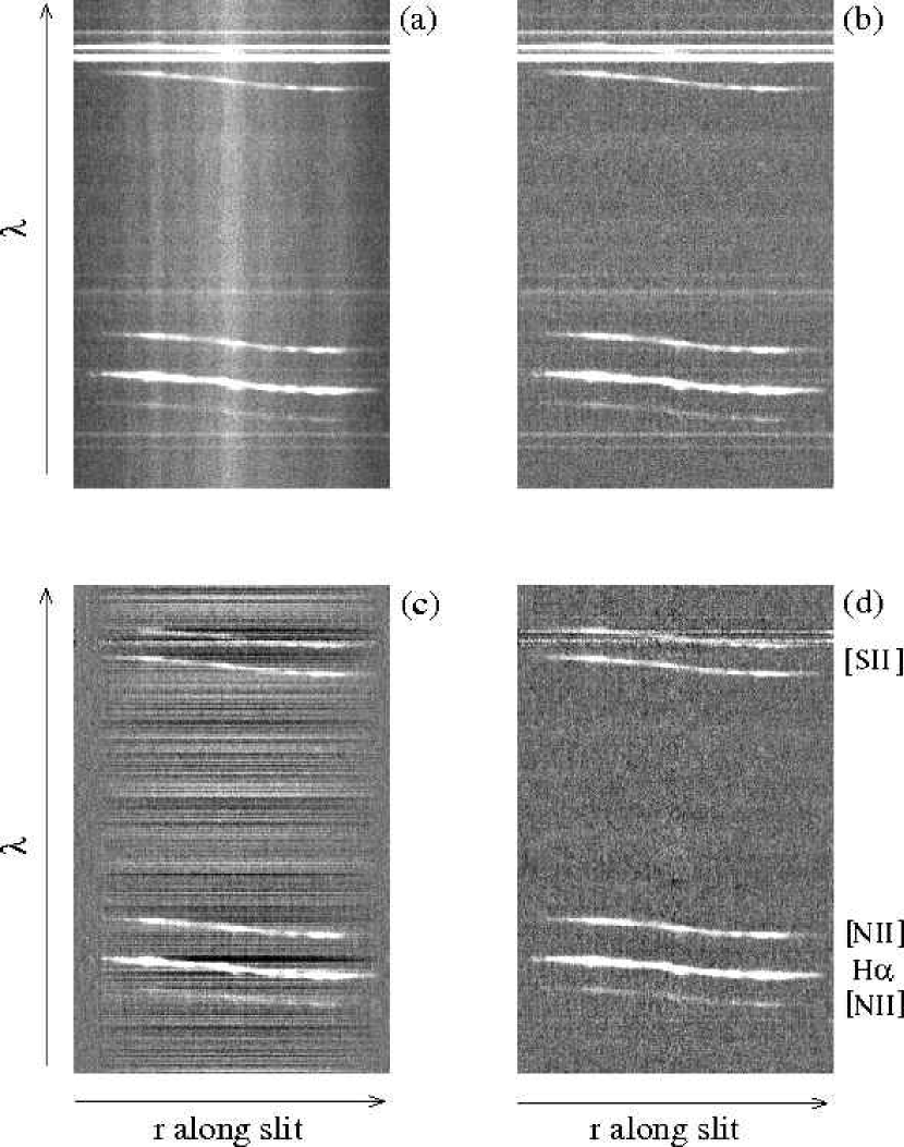
Figure 1.— Demonstration of the template sky line subtraction process for MCG-2-31-017, a galaxy with line emission which fills the slit (we show here only the region with galaxy emission lines; the wavelength range runs approximately from 6610 to 6860 Å). Top panels: spectrum before (a) and after (b) galaxy continuum subtraction. Bottom panels: comparison between standard (c) and template (d) sky subtraction. In (d) the sky lines have been removed by subtracting a sky line template (see text). Different galaxies require, in general, different templates.

Figure 2.— (a) $\rm H\alpha$ RC of MCG-2-31-017, extracted from the sky line-subtracted spectrum in Figure 1c. The dotted lines mark the position of the kinematic center (see § 4, and Figure 3).(b) Same as (a), for Figure 1d. The large residuals present in Figure 1c result in larger error bars in (a) compared to (b).

Figure 3.— Comparison between kinematic (a) and URC (b) folding techniques for MCG-3-05-008. In (a) the RC center is identified by the data point with velocity closest to $V_{\rm sys}=(V_{10}+V_{90})/2$, where $V_{\rm N}$ is the Nth percentile velocity. In (b) the center of symmetry has been determined by fitting a URC model to the unfolded RC. The best-fitting URC (not shown) indicates an offset of $-$34 km s^-1 with respect to the kinematic center (no offset along the spatial direction), and provides a significantly better folding. The solid line in (b) shows the Polyex fit (Equation 2); the dotted line is at the optical radius, where the velocity width is measured. The RC is not deprojected to an edge-on view.

Figure 4.— Distributions of the asymmetry indices for RCs folded according to the URC (solid histogram) or the kinematic (hatched histogram) techniques (see Figure 3). The two indices have been calculated for the optical RCs in our digital archive, for which velocity errors were also available (999 objects). The URC distribution is more centrally concentrated, and does not have a significant tail of high “RC asymmetry”, showing that this algorithm is more effective at minimizing the overall asymmetry of the folded RCs.

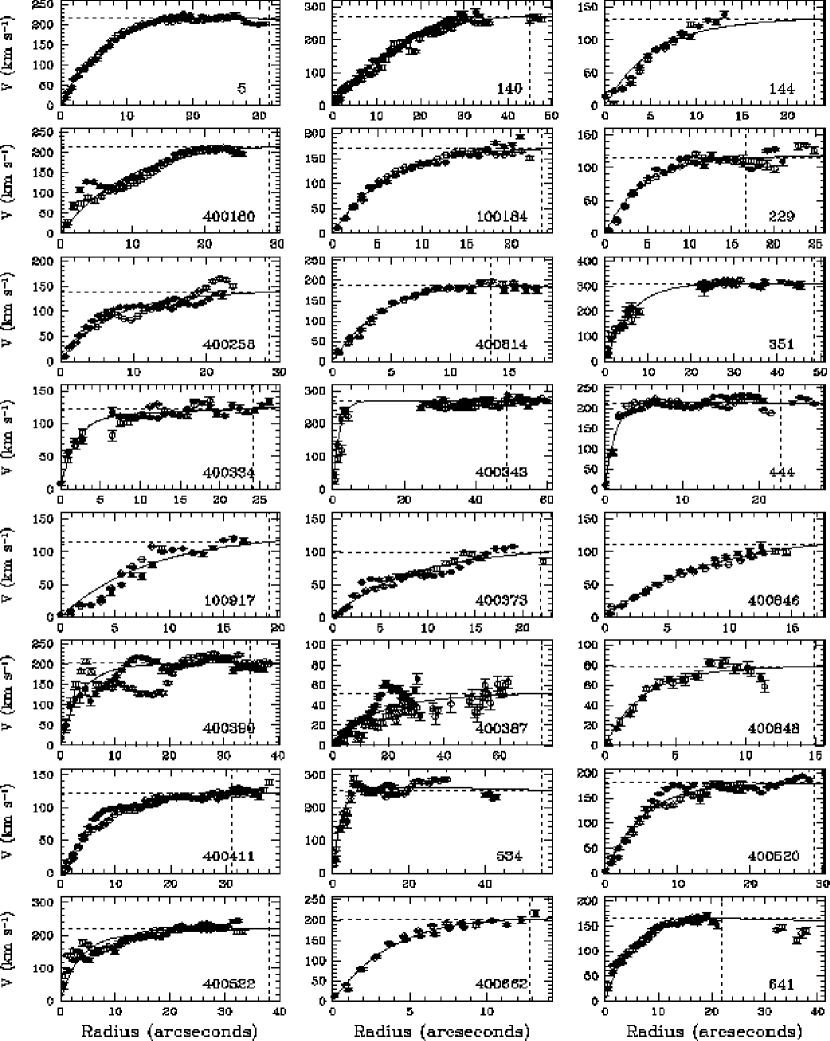
Figure 5.— $\rm H\alpha$ rotation curves, Hanning-smoothed and recorded every other pixel to account for oversampling. The AGC identification code is given in each panel. In one case (AGC 12591) the RC has been extracted from the [NII]$\lambda 6584$ Å emission line. The error bars are formal errors from the Gaussian fits to the peak velocities. The RCs are not deprojected to an edge-on view. The Polyex fit is shown by a solid line; the dotted lines indicate the position of $R_{\rm opt}$ and the adopted half velocity width. We show here only the first page.

Figure 6.— (a) HI content distribution for 715 SFI++ galaxies with optical RC and HI emission profile (solid histogram), and for 27 marginal or non-detections (hatched histogram; the numbers are multiplied by 5 for clarity). (b) Dependence of the RC extent on the HI content for all the objects in (a). The points are running averages, each one including 100 ($x<0.2$), 59 ($x=0.25$), 25 ($0.3<x<0.7$), or 8 ($x=0.97$) measurements; the error bars are Poissonian errors on the mean.

Table 1Palomar Rotation Curve Data.

Galaxy	Other	$\alpha$	$\delta$	T	$R_{\rm opt}$	$R_{max}$	$V_{0}$	$r_{\rm PE}$	$\alpha$	Q	$V_{80}$	$W_{80}$	$V_{PE}$	$W_{PE}$
		J2000	J2000		″	″	km s-1	″			km s-1	km s-1	km s-1	km s-1
(1)	(2)	(3)	(4)	(5)	(6)	(7)	(8)	(9)	(10)	(11)	(12)	(13)	(14)	(15)
5	382-021	00 03 05.5	$-$01 54 51	4B	31.5	30.8	248.4	7.220	$-$0.0289	1	7303	420	7299$\pm$03	418$\pm$05
140	N 52	00 14 40.2	+18 34 55	3	45.1	47.8	374.0	20.576	$-$0.0823	1	5417	491	5414$\pm$08	535$\pm$11
144	456-044	00 15 26.8	+16 14 05	4	22.9	13.1	124.9	5.000	+0.0150	0	5656	211	5640$\pm$18	259$\pm$25
400180	N 64	00 17 30.2	$-$06 49 29	4B	28.9	25.2	249.9	10.695	$-$0.0321	1	7312	398	7312$\pm$09	416$\pm$12
100184	I 1546	00 21 28.8	+22 30 24	4	23.4	22.0	172.5	6.031	+0.0000	1	5820	318	5820$\pm$04	331$\pm$06
229	500-014	00 23 53.4	+28 19 57	3	16.6	24.8	117.9	4.452	+0.0003	1	7235	222	7234$\pm$04	225$\pm$06
400258	M-202038	00 31 13.1	$-$10 28 51	4B	28.6	23.7	128.8	6.158	+0.0185	1	3603	256	3614$\pm$08	274$\pm$11
400814	…	00 31 56.7	$-$10 15 08	4	13.5	17.4	218.5	4.730	$-$0.0331	1	11698	354	11701$\pm$05	359$\pm$07
351	I 34	00 35 36.5	+09 07 25	1B	48.5	45.4	317.7	6.042	$-$0.0036	1	5339	618	5338$\pm$07	606$\pm$10
400334	M-202082	00 40 55.0	$-$13 46 31	3B	24.2	26.2	112.1	1.944	+0.0078	1	8459	240	8463$\pm$04	239$\pm$05
400343	N 217	00 41 33.7	$-$10 01 18	0	48.7	65.9	270.1	1.875	+0.0000	1	3977	554	3976$\pm$10	533$\pm$14
444	519-019	00 42 04.8	+36 48 16	3	22.8	27.1	218.1	1.337	$-$0.0013	1	10650	430	10644$\pm$06	412$\pm$08
100917	…	00 42 11.6	+37 00 56	3	19.2	16.8	112.7	6.998	+0.0350	1	10598	179	10612$\pm$08	223$\pm$10
400373	M-203006	00 45 08.8	$-$09 37 53	4	21.8	22.2	93.0	6.944	+0.0347	1	6110	172	6112$\pm$06	193$\pm$08
400846	M-203014	00 47 25.2	$-$09 51 10	4	16.8	14.6	115.1	7.491	+0.0300	1	5761	182	5761$\pm$06	215$\pm$08
400390	M-203015	00 47 46.2	$-$09 50 05	3B	34.8	38.4	197.3	3.617	+0.0036	1	5767	418	5770$\pm$10	400$\pm$14
400387	UA 14	00 47 46.5	$-$09 53 54	3	75.1	63.1	45.8	13.587	+0.0242	1	1362	098	1358$\pm$10	103$\pm$14
400848	…	00 47 51.9	$-$09 38 46	3	14.9	11.4	74.5	2.565	+0.0103	1	6065	149	6065$\pm$07	154$\pm$10
400411	N 268	00 50 09.5	$-$05 11 37	5B	31.1	37.9	118.1	6.949	+0.0083	1	5492	233	5494$\pm$04	238$\pm$06
534	N 280	00 52 30.2	+24 21 04	3	54.9	43.0	267.6	2.383	$-$0.0024	1	10185	526	10195$\pm$22	489$\pm$30
400520	N 325	00 57 47.5	$-$05 06 45	6	28.8	28.1	184.7	5.402	$-$0.0044	1	5488	344	5487$\pm$04	353$\pm$06
400522	N 329	00 58 01.3	$-$05 04 16	3	38.1	33.1	198.4	3.418	+0.0103	1	5271	436	5267$\pm$10	435$\pm$13
400662	…	00 59 10.3	$-$01 53 57	3	12.8	13.2	232.2	4.202	$-$0.0271	1	15541	364	15546$\pm$07	386$\pm$10
641	N 353	01 02 24.5	$-$01 57 29	2B	21.8	21.0	174.5	4.963	$-$0.0099	1	4107	310	4108$\pm$08	325$\pm$11
410588	M-103075	01 02 48.0	$-$06 24 41	3	24.2	21.5	246.0	13.316	$-$0.0799	1	5775	312	5773$\pm$10	346$\pm$14
410497	384-060	01 02 48.2	$-$01 28 24	3	18.9	26.2	96.3	4.158	+0.0565	1	5876	233	5876$\pm$05	235$\pm$07
410752	…	01 02 55.4	$-$06 24 42	3	13.4	9.3	200.3	1.572	+0.0010	1	13604	380	13603$\pm$08	386$\pm$10
410968	…	01 03 03.7	$-$01 42 49	0	…	…	…	…	0…	…	13991	357	…00	0…
410508	…	01 03 41.2	$-$02 20 15	3	16.0	9.1	309.8	1.922	$-$0.0006	1	21266	568	21266$\pm$31	576$\pm$41
410512	M-103083	01 03 56.2	$-$02 15 44	3	17.9	19.2	233.5	2.408	+0.0120	1	15751	467	15759$\pm$04	483$\pm$05
410518	384-064	01 04 15.0	$-$01 06 51	3B	15.3	12.2	111.8	5.999	+0.0420	1	5420	206	5409$\pm$15	224$\pm$21
410519	…	01 04 21.7	$-$01 31 56	4	16.9	14.5	93.1	7.143	+0.0214	1	5089	137	5084$\pm$05	174$\pm$07

References

- Baes et al. (2003) Baes, M., et al. 2003, MNRAS, 343, 1081
- Bershady et al. (2004) Bershady, M. A., Andersen, D. R., Harker, J., Ramsey, L. W., & Verheijen, M. A. W. 2004, PASP, 116, 565
- Bershady et al. (2005) Bershady, M. A., Andersen, D. R., Verheijen, M. A. W., Westfall, K. B., Crawford, S. M., & Swaters, R. A. 2005, ApJS, 156, 311 (B05)
- Catinella (2005) Catinella, B. 2005, Ph.D. thesis, Cornell Univ.
- Catinella et al. (2005a) Catinella, B., Giovanelli, R., & Haynes, M. P. 2005a, ApJ, submitted
- Catinella et al. (2005b) Catinella, B., Haynes, M. P., & Giovanelli, R., 2005b, in preparation (Paper II)
- Chiba & Yoshi (1995) Chiba, M. & Yoshi, Y. 1995, ApJ, 442, 82
- Courteau (1997) Courteau, S. 1997, AJ, 114, 2402 (C97)
- Dale (1998) Dale, D. A. 1998, Ph.D. thesis, Cornell Univ.
- Dale et al. (1997) Dale, D. A., Giovanelli, R., Haynes, M. P., Scodeggio, M., Hardy, E., & Campusano, L. E. 1997, AJ, 114, 455
- Dale et al. (1998) Dale, D. A., Giovanelli, R., Haynes, M. P. , Scodeggio, M., Hardy, E., & Campusano, L. E. 1998, AJ, 115, 418
- Dale et al. (1999a) Dale, D. A., Giovanelli, R., Haynes, M. P., Hardy, E., & Campusano, L. E. 1999a, AJ, 118 1468
- Dale et al. (1999b) Dale, D. A., Giovanelli, R., Haynes, M. P., Campusano, L. E., & Hardy, E. 1999b, AJ, 118, 1489
- Dale et al. (1999c) Dale, D. A., Giovanelli, R., Haynes, M. P., Campusano, L. E., Hardy, E. & Borgani, S. 1999c, ApJ, 510, L11
- Dale et al. (2001) Dale, D. A., Giovanelli, R., Haynes, M. P., Hardy, E., & Campusano, L. E. 2001, AJ, 121, 1886 (D01)
- Dale & Uson (2003) Dale, D. A., & Uson, J. M. 2003, AJ, 126, 675
- de Vaucouleurs et al. (1991) de Vaucouleurs, G., de Vaucouleurs, A., Corwin, H. G., Buta, R. J., Paturel, G., & Foqué, P. 1991, Third Reference Catalogue of Bright Galaxies (New York: Springer) (RC3)
- Freeman (1970) Freeman, K. C. 1970, ApJ, 160, 811
- Gavazzi et al. (2002) Gavazzi, G., Bonfanti, C., Sanvito, G., Boselli, A., & Scodeggio, M. 2002, ApJ, 576, 135
- Giovanelli & Haynes (2002) Giovanelli, R., & Haynes, M. P. 2002, ApJ, 571, L107
- Giovanelli et al. (1997a) Giovanelli, R., Haynes, M. P., Herter, T., Wegner, G., Salzer, J. J., da Costa, L. N., & Freudling, W. 1997a, AJ, 113, 22
- Giovanelli et al. (1997b) Giovanelli, R., Haynes, M. P., Herter, T., Vogt, N. P., da Costa, L. N., Freudling, W., Salzer, J. J., & Wegner, G. 1997b, AJ, 113, 53
- Haynes & Giovanelli (1984) Haynes, M. P., & Giovanelli, R. 1984, AJ, 89, 758
- Haynes & Giovanelli (1986) Haynes, M. P., & Giovanelli, R. 1986, ApJ, 306, 466
- Haynes et al. (1999) Haynes, M. P., Giovanelli, R., Salzer, J. J., Wegner, G., Freudling, W., da Costa, L. N., Herter, T., & Vogt, N. P. 1999, AJ, 117, 1668
- Koopmann & Kenney (1998) Koopmann, R. A., & Kenney, J. D. P. 1998, ApJ, 497, L75
- Mathewson & Ford (1996) Mathewson, D. S., & Ford, V. L. 1996, ApJS, 107, 97
- Mathewson et al. (1992) Mathewson, D. S., Ford, V. L., & Buchhorn, M. 1992, ApJS, 81, 413
- Navarro et al. (1997) Navarro, J. F., Frenk, C. S., & White, S. D. M. 1997, ApJ, 490, 493
- Nilson (1973) Nilson, P. 1973, Uppsala General Catalogue of Galaxies, Acta Univ. Upsal., Ser. V:A, Vol. 1 (UGC)
- Oke & Gunn (1982) Oke, J. B., & Gunn, J. E. 1982, PASP, 94, 586
- Persic et al. (1996) Persic, M., Salucci, P. , & Stel, F. 1996, MNRAS, 281, 27
- Raychaudhury et al. (1997) Raychaudhury, S., von Braun, K., Bernstein, G. M., & Guhathakurta, P. 1997, AJ, 113, 2046
- Rubin et al. (1999) Rubin, V. C., Waterman, A. H., & Kenney, J. D. P. 1999, AJ, 118, 236
- Solanes et al. (1996) Solanes, J. M., Giovanelli, R., & Haynes, M. P. 1996, ApJ, 461, 609 (SGH96)
- Solanes et al. (2001) Solanes, J. M., Manrique, A., García-Gómez, C., González-Casado, G., Giovanelli, R., & Haynes, M. P. 2001, ApJ, 548, 97
- Springob et al. (2005) Springob, C. M., Haynes, M. P., Giovanelli, R., & Kent, B. R. 2005, ApJS, in press
- Tully & Fisher (1977) Tully, R. B., & Fisher, J. R. 1977, A&A, 54, 661
- Valotto & Giovanelli (2004) Valotto, C., & Giovanelli, R. 2004, AJ, 128, 115
- Vogt (1995) Vogt, N. P. 1995, Ph.D. thesis, Cornell Univ.
- Vogt et al. (2004a) Vogt, N. P., Haynes, M. P., Herter, T., & Giovanelli, R. 2004a, AJ, 127, 3273
- Vogt et al. (2004b) Vogt, N. P., Haynes, M. P., Giovanelli, R., & Herter, T. 2004b, AJ, 127, 3300
- Vorontsov-Velyaminov & Arhipova (1968) Vorontsov-Velyaminov, B. A., & Arhipova, V. P. 1968, Morphological Catalog of Galaxies (Moscow: Moscow State Univ.) (MCG)
- Willick (1999) Willick, J. A. 1999, ApJ, 516, 47
- Zwicky et al. (1961-68) Zwicky, F., Herzog, E., Karpowicz, M., Kowal, C., & Wild, P. 1961-1968, Catalogue of Galaxies and Clusters of Galaxies, Vols. 1-6 (Pasadena: Caltech) (CGCG)