email: [hsafary, nasiri,karami,sobouti]@iasbs.ac.ir
Resonant absorption in dissipative flux tubes
We study the resonant absorption of MHD waves in magnetized flux tubes with a radial density inhomogeneity. Within the approximation that resistive and viscous processes are operative in thin layers surrounding the singularities of the MHD equations, we give the full spectrum of the eigenfrequencies and damping rates of the MHD quasi modes of the tube. Both surface and body modes are analyzed.
Key Words.:
Sun – corona: magnetohydrodynamics (MHD) – Sun: magnetic fields – Sun: oscillations1 Introduction
Ionson (1978) was first to suggest that the resonant absorption of MHD waves in coronal plasmas could be a primary mechanism in coronal heating. Since then, much analytical and numerical work has been done on the subject. Rae and Roberts (1982) investigated both eikonal and differential equation approaches for the propagation of MHD waves in inhomogeneous plasmas. Hollweg (1987a,b) considered a dissipative layer of planar geometry to study the resonant absorption of coronal loops. Poedts et al. (1989, 1990) developed a finite element code to elaborate on the resonant absorption of Alfvén waves in circular cylinders.
Davila (1987) and Steinolfson & Davila (1993) did much work on resonant absorption through resistivity. Ofman et al. (1994) included viscous dissipations in their analysis and concluded that the heating rate due to shear viscosity is comparable in magnitude to the resistive resonant heating. Also, they concluded that the heating caused by compressive viscosity is negligible. Goossens et al. (2002) used the TRACE data of Ofman & Aschwanden (2002) to infer the width of the inhomogeneous layer for 11 coronal loops. Ruderman & Roberts (2002) did similar analysis with the data of Nakariakov et al. (1999). Van Doorsselaere et al. (2004a) used the LEDA code to study the resistive absorption of the kink modes of cylindrical models. They concluded that, when the width of the nonuniform layer was increased, their numerical results differed by as much as 25 from those obtained with the analytical approximation. Van Doorsselaere et al. (2004b) investigated the effect of longitudinal curvature on quasi modes of a typical coronal loop. They found that the frequencies and damping rates of ideal quasi modes were not influenced much by the curvature. Andries et al. (2005) studied the effect of density stratification on coronal loop oscillations, and conclude that longitudinal mode numbers are coupled due to the density stratification.
In the absence of resonance, Edwin & Roberts (1983) and Roberts et al. (1984) gave a comprehensive account of the theoretical and physical concepts related to coronal oscillations. Karami et al. (2002; hereafter paper I) studied the full spectrum of MHD modes of oscillations in zero- magnetic flux tubes with discontinuous Alfvén speeds at the tube’s surface. In the vicinity of singularity, field gradients are large. Recognizing this, Sakurai et al. (1991a, b) and Goossens et al. (1992, 1995) developed a method to analyze dissipative processes in such regimes and to neglect them elsewhere.
Here we combine the two techniques of paper I and of Sakurai et al. (1991a) to obtain the resonant damping rates for the full spectrum of the normal modes of magnetic flux tubes.
2 Equations of motions
The linearized MHD equations for a zero-, but resistive and viscous, plasma are
| (1) |
| (2) |
where and are the Eulerian perturbations in the velocity and the magnetic fields; , , , and are the mass density, the electrical conductivity, the viscosity and the speed of light, respectively. The simplifying assumptions are:
-
•
Under coronal conditions gas pressure is negligible (zero- ).
-
•
Density scale heights are much larger than the dimensions of flux tube, so that the gravity stratification is negligible.
-
•
The tube geometry is a circular cylinder with coordinates (,,).
-
•
There is a constant magnetic field along the axis, .
-
•
The equilibrium is static.
-
•
There is no initial steady flow inside or outside of the tube.
-
•
Viscous and resistive coefficients, and respectively, are constants.
For a variable density, , a singularity develops wherever the local Alfvén frequency becomes equal to the global frequency of the mode. The relevant radial wave number vanishes and resonant absorption takes place. Let us denote the radius of the tube by and a radius beyond which the resonance occurs by . The thickness of the inhomogeneous layer, , will be assumed to be small and will be arbitrarily taken to be of the order . The choice of density profile is also unimportant. We will assume two constant densities, in and in , interconnected with a linearly varying profile in .
In the remainder of this section the following steps are taken:
- a)
- b)
- c)
-
Interior and exterior solutions are connected by requiring the jumps in (b) to be equal to the differences in (a). This gives an analytical expression for a complex dispersion relation to be solved for the frequencies and the damping rates.
2.1 Interior and exterior solutions
From paper I, in the absence of dissipations, all components of and the transverse components of are expressible in terms of only. The latter, in turn, is the solution of a second order differential equation. Thus,
| (3) | |||
| (4) |
| (5) |
where , and is the local Alfvén speed. Here, we have assumed an exponential , and dependence, for any component of and .
In the interior region, , solutions of Eq. (3) are
| (6) |
where and are Bessel and modified Bessel functions of the first kind, respectively. In the exterior region, , the waves should be evanescent. Solutions are
| (7) |
where is the modified Bessel function of the second kind.
2.2 Dispersion relation and damping
From Sakurai et al. (1991a), Goossens et al. (1992, 1995), and Erdélyi et al. (1995), the jump conditions across the boundary for and are
| (8) | |||
| (9) |
where is the radius at which the singularity occurs and , , and . Substituting the fields of Eqs. (5), (6) and (7) in jump conditions and eliminating the arbitrary amplitudes of the waves, as foreseen initially inside and outside of the boundary layer, gives the dispersion relation
| (10) |
where
| (11) | |||
| (12) |
In principle is expected to be found as a solution of Eqs. (10-12). In particular for , Eq. (10) can be expanded about to give
| (13) |
The results for surface waves are the same as Eqs. (10)- (13), except that is replaced by everywhere. This completes the formal solutions of and . Further analytical progress is still possible when the inhomogeneous layer is thin enough.
3 Thin boundary approximation
Here we assume . Equation (10) reduces to . For body waves, the latter is studied in ample detail in paper I. There, a trio of wave numbers , corresponding to , and directions, is assigned to each mode. From Eq. (13) the corresponding damping rate becomes
| (14) | |||||
Again the results for surface waves are the same as those for body waves except that is replaced by . The two waves exhibit differences, for and behave differently at the boundary. We also note that each surface mode is designated by only two wave numbers, corresponding to and directions, respectively.
4 Numerical results
As typical parameters for a coronal loop, we adopt radius = km, length = km, gr cm-3, , G. For these parameters one finds km s-1, km s-1 and rad s-1.
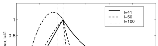
In Fig. 1 the magnetic field component, , for , and , are plotted versus . They are normalized to . The segment of the plot in is from the interior solutions of Eq. (6), while the segment in is from the exterior solutions of Eq. (7). Slopes are discontinuous at . Actually, the correct location of the discontinuities is the point of singularity, . Its appearance at is an artifact caused by extrapolating the interior solutions to cover the boundary layer, rather than using the exact solutions there. As increases, the maximum wave amplitude moves towards the tube axis and away from the inhomogeneous layer.
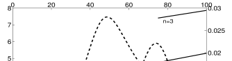
In Fig. 2, the frequencies and the damping rates are plotted versus . The frequencies increase with increasing and/or . For and , damping rates exhibit maxima at and , respectively. For there is only a declining branch towards higher values. Our explanation for the occurrence of maxima in damping rates is the localization of the maximum amplitude of a wave within the resonant layer, where the dissipation is expected to be the highest. As Fig. 1 shows, this maximum moves away from that layer at both lower and higher values.
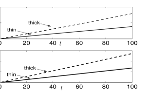
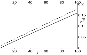
For surface waves, specified by two mode numbers , and are plotted in Figs. 3 and 4. Both frequencies and damping rates show a monotonous increase with . Two tube radii, , are considered here. The frequencies and damping rates of the thicker tube are almost double those of the thinner tube. This is expected, because in the limit of thin tubes, both and are proportional to (see, e. g., Van Doorsselaere et al. 2004). The frequencies of the surface waves of Fig. 3 and the body frequencies of Fig. 2 both behave similarly. This is because of the similar behavior of and at small arguments. In physical terms this means, at least in the thin tube approximation, the surface and the - fundamental body waves contribute in equal manner to the heating mechanism; they both dump the bulk of their energies near the tube surface, and perhaps both are excited with comparable amplitudes and energies. The is the number of oscillations taking place before a wave is completely attenuated. For thick and thin tubes, and , this number is about and , respectively. An observed value of Nakariakov et al. (1999) from TRACE data is about . Those of Goossens et al. (2002) from the same source range from - corresponding, according to the authors, to various values of , , and .
5 Summary
We studied the MHD quasi modes of coronal loops. On the assumption that ohmic and viscous dissipations are operative within a thin boundary layer, we obtained an analytic dispersion relation and solved it numerically for the mode frequencies and the damping rates. For realistic values of the initial parameters thickness- to- height ratio of the loop, the density contrast with the background medium, and the equilibrium magnetic field- our numerical values agree with those obtained from observations. As the longitudinal wave number increases, the maximum amplitude of the body eigenmodes shifts away from the resonant layer and causes a decrease in damping rates. Its behavior with increasing radial wave number is not, however, all that straightforward. In additional, we have shown that body and surface modes may contribute equally to the heating of coronal loops.
Acknowledgements.
The authors wish to thank Professors Robert Erdélyi and, Marcel Goossens for valuable consultations. Elaborate and meticulous comments of the referee has significantly improved the content and the presentation of the paper. This work was supported by the Institute for Advanced Studies in Basic Sciences (IASBS), Zanjan.References
- (1) Andries, J., Goossens, M., Hollweg, J. V., Arregui, I., & Van Doorsselaere, 2005, A&A, 430, 1109
- (2) Davila, J. M. 1987, ApJ, 317, 514
- (3) Edwin, P. M., & Roberts, B. 1983, Sol. Phys., 88, 179
- (4) Erdélyi, R., Goossens, M., & Ruderman, M. S. 1995, Sol. Phys., 161, 123
- (5) Goossens, M., Hollweg, J. V., & Sakurai, T. 1992, Sol. Phys., 138, 233
- (6) Goossens, M., Ruderman, M. S., & Hollweg, J. V. 1995, Sol. Phys., 157, 75
- (7) Goossens, M., Andries, J., & Aschwanden, M. J. 2002, A&A, 394, L39
- (8) Hollweg, J. V. 1987a, ApJ, 312, 880
- (9) Hollweg, J. V. 1987b, ApJ, 320, 875
- (10) Ionson, J. A. 1978, ApJ, 226, 650
- (11) Karami, K., Nasiri, S. & Sobouti, Y. 2002, A&A, 396, 993 (Paper I)
- (12) Nakariakov, V. M., Ofman, L., Deluca, E. E., Roberts, B., & Davila, J. M. 1999, Science, 285, 862
- (13) Ofman, L., Davila, J. M., & Steinolfson, R. S. 1994, ApJ, 421, 360
- (14) Ofman, L., & Aschwanden, M. J. 2002, ApJ, 576, L153
- (15) Poedts, S., Goossens, M., & Kerner, W. 1989, Sol. Phys., 123, 83
- (16) Poedts, S., Goossens, M., & Kerner, W. 1990, ApJ, 360, 279
- (17) Rae, I. C., & Roberts, B. 1982, MNRAS, 201, 1171
- (18) Roberts, B., Edwin, P. M., & Benz, A. O. 1984, ApJ, 279, 857
- (19) Ruderman, M. S. & Roberts, B. 2002, ApJ, 577, 475
- (20) Sakurai, T., Goossens, M., & Hollweg, J. V. 1991a, Sol. Phys., 133, 247
- (21) Sakurai, T., Goossens, M., & Hollweg, J. V. 1991b, Sol. Phys., 133, 227
- (22) Steinolfson, R. S., & Davila, J. N. 1993, ApJ, 415, 354
- (23) Van Doorsselaere, T., Andries, J., Poedts, S., & Goossens, M. 2004a, ApJ, 606, 1223
- (24) Van Doorsselaere, T., Debosscher, A., Andries, J., & Poedts, S. 2004b, A&A, 424, 1065