Abstract

Numerical simulations of atmospheric turbulence and AO wavefront correction are performed to investigate the timescale for fringe motion in optical interferometers with spatial filters. These simulations focus especially on partial AO correction, where only a finite number of Zernike modes are compensated. The fringe motion is found to depend strongly on both the aperture diameter and the level of AO correction used. In all of the simulations the coherence timescale for interference fringes is found to decrease dramatically when the Strehl ratio provided by the AO correction is $\mathrel{\hbox to0.0pt{\lower 3.0pt\hbox{$\mathchar 536\relax$}}\raise 2.0pt\hbox{$\mathchar 316\relax$}\hss}30\%$. For AO systems which give perfect compensation of a limited number of Zernike modes, the aperture size which gives the optimum signal for fringe phase tracking is calculated. For AO systems which provide noisy compensation of Zernike modes (but are perfectly piston-neutral), the noise properties of the AO system determine the coherence timescale of the fringes when the Strehl ratio is $\mathrel{\hbox to0.0pt{\lower 3.0pt\hbox{$\mathchar 536\relax$}}\raise 2.0pt\hbox{$\mathchar 316\relax$}\hss}30\%$.

1 Introduction

The field of astronomical interferometry has matured over the past two decades with a substantial number of interferometric arrays being constructed around the world[1]. The majority of the interferometric instruments at existing arrays utilise pupil-plane Michelson beam combination. These instruments probe the structure on much smaller angular scales than can be resolved by the individual telescopes which make up the array, and the light which is useful for an interferometric measurement typically resides within a region which is unresolved by the individual telescopes (so the parts of an astronomical source which are studied interferometrically typically lie within a single diffraction-limited point spread function for one of the telescopes making up the interferometric array). It is common at such interferometers for the incoming wavefronts to be spatially filtered by using a pinhole or a single-mode fibre to select light from the central core of the Airy pattern in the image plane of each telescope, and to exclude all light from the periphery of the Point-Spread Function (PSF)[2, 1], as this light would decrease the signal-to-noise ratio for measurements of the fringe visibility.

Optical wavefronts from an astronomical source passing through the Earth’s atmosphere are perturbed by fluctuations in air density and water vapour density[3] resulting in rotation of the phase of the optical wavefronts. Experimental measurements indicate that the spatial and temporal power spectra of these fluctuations are usually well fit by Kolmogorov models[4, 5, 6] for spatial scales between the inner and outer scales of turbulence.

If there are atmospherically-induced wavefront perturbations across one of the telescope apertures in an interferometric array there may be a significant reduction in the on-axis Strehl ratio measured at that telescope, with only a fraction of the light falling into an on-axis Airy disk. This results in a reduction in the flux entering a spatial filter positioned on the optical axis, as well as fluctuations in the optical phase of that light. The flux reduction has been studied elsewhere[7, 1], and so I concentrate here on the fluctuations in the optical phase found after the spatial-filtering process.

For an optical interferometer formed from two telescopes of finite diameter observing a source which is unresolved by the individual telescopes, the contribution of atmospheric turbulence can be split into two components:

1. The difference in the mean optical path for the two different light paths to the star through the two apertures – the differential piston mode[8] Zernike[9] component

2. The wavefront corrugations over each individual telescope aperture of the interferometer (the higher order Zernike modes)

If each telescope has a spatial filter, then both of the components listed above will affect the timescales over which the fringes move (and hence those over which fringe measurements must be made). The contribution from component 2 results from the strong coupling of the high-order Zernike modes for wavefronts in the telescope aperture plane to the optical phase output from the spatial filter (as is customary, I use the term “optical phase” to indicate the phase of the monochromatic optical wavefronts measured relative to the wavefront phase before the light was perturbed by the atmosphere or optical instrumentation). An adequate analytical model for the contribution of this to the timescale for fringe motion in an interferometer has not yet been developed. This has forced most previous authors either to limit their discussions of fringe motion to small apertures (e.g. Ref. [10]) or to ignore the effect of term 2 above even for large apertures[8, 11], which would be a valid assumption for the case of ideal adaptive optics (AO) correction providing Strehl ratios of $100\%$.

The numerical simulations presented here address the timescale for fringe motion in an interferometer with large apertures and only partial AO correction. Although simulations such as these have been performed previously when optimising the design of interferometers, as far as I am aware detailed results have not been published in the literature. In order to keep the results as general as possible, the atmosphere was modelled using unchanging Kolmogorov phase screens blown past in a wind-scatter model[12], and the AO correction in the simulations was restricted to compensation of a finite number of Zernike modes.

2 Simulation method

Simulations were developed to investigate the motion of interference fringes in a two-element optical interferometer. The optical modelling was limited to one pupil plane and one image plane and the wavefront was sampled as complex numbers in a rectangular grid of points fine enough to avoid aliasing errors. Transformations from the pupil plane to the image plane were performed by applying an FFT to the grid of points. Input wavefront perturbations were provided by two Taylor screens introducing Kolmogorov phase perturbations with a large outer scale ($>1000r_{0}$ – further details of the simulations can be found in Ref. [13]). Both screens moved at the same speed but at an angle of $120^{\circ}$ with respect to each other (chosen arbitrarily). This arrangement provided a speckle coherence timescale $\Delta_{\tau}$ (see Ref. [12]) which was essentially independent of aperture diameter. The results are not expected to depend critically on the dispersion in the wind velocities (the wind dispersion only strongly effects the speckle pattern properties in telescopes without AO[12]), but for realistic simulations of existing interferometers researchers are encouraged to select wind velocity profiles which match the conditions above their interferometer as closely as possible. The time unit in the simulations was defined as the time taken for each phase screen to move by the coherence length $r_{0}$ for the full atmosphere. The simulations were repeated at discrete time-steps separated by $1/10$th of a time unit.

The wavefront perturbations introduced by the atmosphere were calculated at a grid of points at fixed locations in the telescope pupil plane, with the values being based on linear interpolation between the grid points making up the moving Taylor screen arrays to minimise aliasing effects.

Experience from previous simulations[13] and from real interferometers indicates that the fringe motion in an interferometer is only affected significantly by wavefront corrugations on the individual telescopes when the image breaks up into multiple speckles. Each speckle in a multi-speckle image has a random (wavelength-dependent) phase rotation relative to the mean piston phase of the wavefronts in the pupil plane. Adjustment of Zernike modes above the piston mode (e.g. AO correction) causes changes to the image plane speckle pattern, resulting in changes to the phases measured in the image plane even if the pupil-plane piston mode is unaffected. The simulations presented here will investigate the effects of the residual wavefront errors after partial AO correction on the phases measured in an image-plane spatial filter.

The AO correction of the wavefront perturbations was simulated by numerically correcting the lowest Zernike modes in the pupil plane (excluding piston). Care was taken to ensure that the pupil plane piston mode component was not changed during this correction process. Eight levels of AO correction were simulated as listed in Table 1.

Table 1: Models for AO wavefront correction

Model	Highest Zernike mode corrected ($j$)	Diameter $D_{j}$†
$1$	$3$	$3.3r_{0}$
$2$	$6$	$5.2r_{0}$
$3$	$10$	$6.9r_{0}$
$4$	$15$	$8.6r_{0}$
$5$	$21$	$10r_{0}$
$6$	$28$	$12r_{0}$
$7$	$36$	$13r_{0}$
$8$	$45$	$15r_{0}$

†	The aperture diameter where the variance of the wavefront phase would be $1$ rad2

The long exposure on-axis Strehl ratio $R$ is described by[7]:

$$R\geq\exp(-\sigma^{2})$$ (1)

where $\sigma^{2}$ is the residual variance in the wavefront phase in the on-axis direction. If $\sigma^{2}<1$ rad² after AO correction, the point-spread function for the telescope will be almost diffraction-limited with a Strehl ratio of more than $37\%$, and the measured optical phase after spatial filtering is expected to closely match the mean piston-mode component. A minimum diameter $D_{j}$ was defined as that where the residual phase variance $\sigma^{2}$ was $1$ rad², given by:

$$D_{j}/r_{0}=\left(a_{j}\right)^{-3/5}$$ (2)

where $a_{j}$ is the numerical coefficient in the $j$th Zernike-Kolmogorov residual error formula of Table IV from Ref. [9]. Values of $D_{j}$ are included in Table 1 for each of the models. Based on these values, a range of aperture diameters between $4r_{0}$ and $20r_{0}$ were chosen for the all simulations presented here.

In order to reduce the complexity of the simulations, only one arm of the interferometer was modelled. In an interferometer with widely-separated apertures the wavefront corrugations measured at the two apertures will be uncorrelated, and the RMS fringe phase change in the interferometer will be $\sqrt{2}$ times greater than the RMS change in optical phase measured at either one of the telescopes. The results calculated here for a single telescope can thus be readily extrapolated to the case of a long-baseline interferometer.

After AO correction, the optical wavefronts were spatially filtered by summing over a uniform circular disk in the telescope image plane. The circular disk used had a diameter corresponding to an angle of $\lambda/D$ on the sky (typical for pinhole or single-mode fibre spatial filters[2]), where $\lambda$ was the mean wavelength for the observation and $D$ was the aperture diameter used. This summed flux was used for the remainder of the simulation.

In an optical interferometer operating with a finite optical bandpass, interference fringes are only found over a narrow range of optical path difference (a narrow range of differential optical delay between the two telescopes and the beam combiner). The maximum level of interference is found when the optical delay (optical path) along one arm of the interferometer is adjusted so that the gradient of optical phase difference with wavelength is at a minimum. This delay setting occurs when the reciprocal of the group velocity integrated along the both optical paths from the star is equal, and is called the group delay.

The optical phase delay was tracked in the simulations using a three-stage process designed to emulate what might be done at a real interferometer:

1. The phase difference between light in two closely-spaced wavelength channels was used to calculate a group delay.

2. A change in the optical delay in one interferometer arm was simulated by rotating the phases in each channel, subtracting the group delay offset measured in 1. (using the $\frac{2\pi}{\lambda}$ factor between phase and optical path to correctly take account of the wavelength $\lambda$ of each channel).

3. An average phase was calculated for the two channels (averaging vector representations of the electric field to avoid phase-wrapping errors).

4. The group delay offset subtracted in 2. was added back to give an unwrapped phase (corresponding to $2\pi$ times the optical path offset measured in wavelengths).

In these simulations the two wavelengths used were separated by $1\%$ of the mean wavelength, a sufficiently narrow bandpass that the effect of the variation in the light path through the atmosphere with wavelength due to atmospheric refraction can be ignored. Care was taken to ensure that the same sampling grid was used in the image plane for both wavelengths, that the pupil plane representations of the wavefronts were truncated at the same aperture diameter, and that the wavelength difference was correctly taken into account when interpolating the wavefront perturbations from the atmospheric Taylor screens.

3 Results

In order to separate the effects of higher Zernike modes from the piston mode across the telescope aperture, the piston mode measured in the pupil plane was subtracted from the phases measured at the spatial filter for each of the simulations. The RMS of the result is a measure of the phase jitter introduced by wavefront corrugations across the simulated telescope apertures. The RMS jitter in a two-element interferometer is $\sqrt{2}$ times larger than the jitter in the unwrapped phase for a single telescope, and is shown for simulations of $8192$ time-steps in Fig. 1.

Figure 1: The RMS jitter in the optical phase in an interferometer with spatial filters, plotted against aperture diameter. The jitter results from wavefront corrugations in the telescope aperture plane. Each line connects models with a given level of AO correction, and is labelled with the number of Zernike modes which have been suppressed. The phase jitter plotted represents the RMS difference between the optical phase calculated for that model and the phase delay after ideal AO correction.

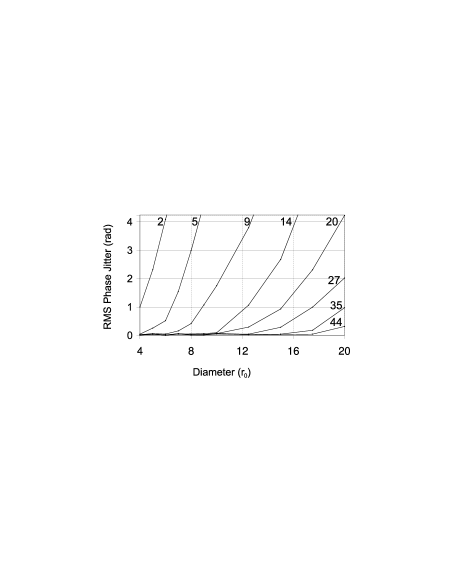
Phase jitter in the interference fringes will significantly degrade the interferometric performance when it reaches $\sim 1$ rad RMS. In these simulations this level of phase jitter is only reached if the aperture diameter is significantly greater than $D_{j}$ (see Table 1), corresponding to AO Strehl ratios significantly less than $37\%$. It is clear, however, that the phase jitter does become significant with large telescope apertures and non-ideal AO correction, and should thus be taken into account in signal-to-noise calculations for interferometer performance.

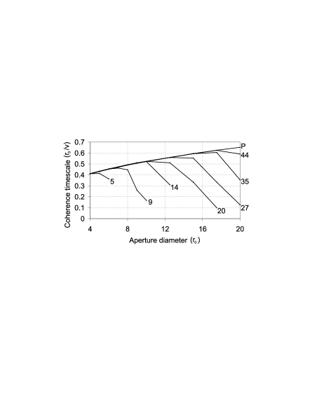
If the phase jitter is $\mathrel{\hbox to0.0pt{\lower 3.0pt\hbox{$\mathchar 536\relax$}}\raise 2.0pt\hbox{$\mathchar 318\relax$}\hss}1$ rad RMS, then the temporal frequency spectrum of the phase jitter will affect the optimum exposure time for fringe observations in the interferometer. Temporal structure functions of the total optical phase (including both the phase jitter and the piston mode) were calculated for each model of AO wavefront correction and each aperture size. From these structure functions the timescale for the phase to change by $1$ rad in the interferometer was calculated using linear interpolation. This corresponds to the coherence timescale for the fringe phase in an optical interferometer having this level of AO correction. The calculated timescales are shown in Fig. 2 for all aperture sizes where the timescale was sufficiently long to allow meaningful interpolation from the sampled structure function.

Figure 2: The coherence timescale for the optical phase for a range of aperture diameters and different levels of AO correction. The labels on the lines indicate the number of Zernike modes corrected from tip-tilt upwards. The curve labelled “P” corresponds to the coherence timescale of the piston mode, indicating the result expected for ideal AO correction. The endpoint of each curve is determined by the time-resolution of the simulations performed.

I will now look at how the signal-to-noise in an interferometer can be optimised, allowing the usage of observing time to be minimised. I will assume here that there are limits on the instrumentation available (so that, for example, the level of AO correction cannot be arbitrarily increased in order to maximise the signal-to-noise ratio), and that the seeing conditions are fixed. A commonly used approach to improving the signal-to-noise ratio under these constraints at astronomical interferometers is to adjust the telescope aperture diameter (e.g. the tip-tilt corrected COAST apertures were stopped down to 14cm for the first interferometric imaging observations[14]). In order to maintain the same level of AO correction with a reduced aperture diameter, the AO system must clearly be optically matched to the new aperture size.

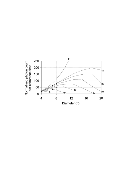
The signal-to-noise ratio for tracking the phase of interference fringes in an interferometer is determined by the number of photons arriving per coherence time (where the coherence time is again the RMS time taken for the fringe phase to change by one radian). The photon count entering the spatial filter per coherence time was calculated for each aperture diameter and each level of AO correction, and these are plotted in Fig. 3. The drop in the photon counts for large aperture sizes and partial AO correction is largely due to the increased phase jitter and decreased coherence timescale for large aperture sizes (see Figs. 1 and 2). For each level of AO correction, the aperture diameter which provides the optimum signal-to-noise is marginally larger than $D_{j}$ from Table 1. The Strehl ratio provided by the AO system is $\sim~{}30\%$ at the optimum aperture size in each case – for simulations with Strehl ratios lower than this, decreasing the aperture size would increase the photon count through the spatial filter per coherence time if the AO system was still matched to the aperture diameter.

Figure 3: The photon count through the spatial filter per coherence timescale normalised so that a diffraction-limited aperture of diameter $r_{0}$ would give unity. The labels on the lines indicate the number of Zernike modes corrected from tip-tilt upwards. The curve labelled “P” corresponds to the result expected for ideal AO correction.

Real AO systems do not perfectly compensate each Zernike mode (particularly for faint off-axis reference stars), so additional simulations were undertaken to determine the effect of noise in the Zernike mode compensation on the RMS phase jitter. Every AO system has different noise properties, and the calculation of the likely noise spectrum from a real AO system is extremely complex. To keep the simulations as simple and general as possible, the noise was simply modelled as being a small fraction of the atmospheric corrugations. For example, in one simulation each of the corrected Zernike modes was reduced to $10\%$ of the original amplitude, while uncorrected modes were not adjusted. $44$ Zernike modes after piston were corrected in all of these simulations, each mode being reduced to between $5\%$ and $50\%$ of its original amplitude, depending on the simulation. Aperture sizes from $4r_{0}$ to $20r_{0}$ were investigated. Although the simulations presented here will not be quantitatively accurate for any particular interferometer, they will provide a qualitative description of what happens at all AO corrected interferometers.

In all of the simulations the RMS phase jitter increased dramatically whenever the Strehl ratio was $\mathrel{\hbox to0.0pt{\lower 3.0pt\hbox{$\mathchar 536\relax$}}\raise 2.0pt\hbox{$\mathchar 316\relax$}\hss}~{}30\%$ (corresponding to $\mathrel{\hbox to0.0pt{\lower 3.0pt\hbox{$\mathchar 536\relax$}}\raise 2.0pt\hbox{$\mathchar 318\relax$}\hss}~{}1$ rad RMS wavefront error in the aperture plane). In real AO systems the temporal properties of the noise in the correction of Zernike modes is dependent on the bandwidth of the AO system. When the Strehl ratio falls below $30\%$ we can expect the coherence timescale for the fringes in the interferometer to be determined by the temporal properties of the AO system, even if the AO system does not introduce fluctuations in the aperture plane piston mode.

4 Conclusions

Numerical simulations of atmospheric turbulence and AO wavefront correction were performed to investigate the timescale for fringe motion in optical interferometers with spatial filters. The fringe motion was found to depend strongly on both the aperture diameter and the level of AO correction used. In all of the simulations the coherence timescale for interference fringes was found to decrease dramatically when the Strehl ratio provided by the AO correction was $\mathrel{\hbox to0.0pt{\lower 3.0pt\hbox{$\mathchar 536\relax$}}\raise 2.0pt\hbox{$\mathchar 316\relax$}\hss}30\%$. For AO systems which give perfect compensation of a limited number of Zernike modes, the optimum aperture size for fringe phase tracking was calculated and found to be dependent on the number of modes corrected. For AO systems which provide noisy compensation of Zernike modes (but are perfectly piston-neutral), the noise properties of the AO system were found to determine the coherence timescale of the interference fringes when the Strehl ratio is $\mathrel{\hbox to0.0pt{\lower 3.0pt\hbox{$\mathchar 536\relax$}}\raise 2.0pt\hbox{$\mathchar 316\relax$}\hss}30\%$. These results highlight the need for time-resolved modelling of the wavefront corrugations and fringe phase in existing AO-corrected interferometers in order to fully understand the jitter seen in the phase of the interference fringes.

References

- [1] J. D. Monnier, “Optical interferometry in astronomy,” in Reports of Progress in Physics, 66, pp. 789–857 (2003), astro-ph/0307036.
- [2] J. W. Keen, D. F. Buscher, and P. J. Warner, “Numerical simulations of pinhole and single-mode fibre spatial filters for optical interferometers,” Monthly Notices of the Royal Astronomical Society 326, 1381–1386 (2001), astro-ph/0106442.
- [3] F. Roddier, “The effects of atmospheric turbulence in optical astronomy,” in Progress in optics. Volume 19. Amsterdam, North-Holland Publishing Co., pp. 281–376 (1981).
- [4] V. I. Tatarski, Wave Propagation in a Turbulent Medium (McGraw-Hill, New York, 1961).
- [5] A. N. Kolmogorov, “Dissipation of energy in the locally isotropic turbulence,” Comptes rendus (Doklady) de l’Académie des Sciences de l’U.R.S.S. (Moscow), 32, 16–18 (1941).
- [6] A. N. Kolmogorov, “The local structure of turbulence in incompressible viscous fluid for very large Reynold’s numbers,” Comptes rendus (Doklady) de l’Académie des Sciences de l’U.R.S.S. (Moscow), 30, 301–305 (1941).
- [7] T. Fusco, and J. Conan, “On- and off-axis statistical behavior of adaptive-optics-corrected short-exposure Strehl ratio,” J. Opt. Soc. Am. A 21, 1277–1289 (2004).
- [8] J. Conan, G. Rousset, and P. Madec, “Wave-front temporal spectra in high-resolution imaging through turbulence,” J. Opt. Soc. Am. A 12, 1559–1570 (1995).
- [9] R. J. Noll, “Zernike polynomials and atmospheric turbulence,” J. Opt. Soc. Am. 66, 207–211 (1976).
- [10] D. F. Buscher, “Getting the most out of C.O.A.S.T.” Ph.D. thesis, Cambridge University (1988). URL http://www.mrao.cam.ac.uk/~dfb/publications/dfbphd.pdf.
- [11] L. A. D’Arcio, “Selected aspects of wide-field stellar interferometry,” Ph.D. thesis, Technische Universiteit Delft (1999).
- [12] F. Roddier, J. M. Gilli, and G. Lund, “On the origin of speckle boiling and its effects in stellar speckle interferometry,” Journal of Optics 13, 263–271 (1982).
- [13] R. N. Tubbs, “Seeing timescales for large-aperture optical/infrared interferometers from simulations,” in Proc. SPIE Vol. 5491, New Frontiers in Stellar Interferometry, W. Traub Ed., 1240–1248 (2004).
- [14] J. E. Baldwin, M. G. Beckett, R. C. Boysen, D. Burns, D. F. Buscher, G. C. Cox, C. A. Haniff, C. D. Mackay, N. S. Nightingale, J. Rogers, P. A. G. Scheuer, T. R. Scott, P. G. Tuthill, P. J. Warner, D. M. A. Wilson, and R. W Wilson, “The first images from an optical aperture synthesis array: mapping of Capella with COAST at two epochs,” Astronomy and Astrophysics 306, L13–16 (1996).