The high-velocity clouds and the Magellanic Clouds

From an analysis of the sky and velocity distributions of the high-velocity clouds (HVCs) we show that the majority of the HVCs has a common origin. We conclude that the HVCs surround the Galaxy, forming a metacloud of $\sim 300\mbox{ kpc}$ in size and with a mass of $\sim 3\times 10^{9}\,\mathrm{M}_{\sun}$, and that they are the product of a powerful “superwind” (about $10^{58}\mbox{ ergs}$), which occurred in the Magellanic Clouds about $570\mbox{ Myr}$ ago as a consequence of the interaction of the Large and Small Magellanic Clouds. The HVCs might be magnetic bubbles of semi-ionized gas, blown from the Magellanic Clouds around $570\mbox{ Myr}$ ago, that circulate largely through the halo of the Galaxy as a stream or flow of gas.

On the basis of the connection found between the HVCs and the Magellanic Clouds, we have constructed a theoretical model with the purpose of computing the orbits of a sample of test particles representing the HVCs, under the gravitational action of the Galaxy and the Magellanic Clouds. The orbits of the Large and Small Magellanic Clouds have been traced backwards in time to estimate the position and velocity of the Clouds at the time of the collision between the two Clouds, and to infer the initial conditions of the HVCs. The model can reproduce the main features of position and velocity distributions of the HVCs, like the overall structure and kinematics of the Magellanic Stream. The initial velocities of the HVCs were the result of velocities of expansion that permitted the escape of the HVCs from the Magellanic Clouds plus the systemic velocity of the Magellanic Clouds at the time of the collision. With these initial conditions, the Galactic gravitational potential induced differential rotations or shearing motions that elongated the cloud of HVCs in the orbital direction, forming the rear and front parts of the Magellanic stream. The population of HVCs is centered around the Magellanic Clouds. The eccentric position of the Sun within the cloud of HVCs explains the asymmetries between the sky distributions of the HVCs of the northern Galactic hemisphere and those of the southern Galactic hemisphere.

In the light of the model we analyze the effects that the passage of the HVC flow through the Galactic disk has produced on the interstellar medium. The effects of the HVC flow can account for many observational details such as the Galactic warp, HI shells and supershells in the gaseous layer of the outer parts of the Milky Way. The Galactic disk was target of numerous impacts of HVCs in the course of the last $400\,\mbox{Myr}$, accumulating mass at the average rate of approximately $0.6\,\mathrm{M}_{\sun}$ per year. The events of this period may be regarded as landmarks in the evolutionary history of the Milky Way.

1 Introduction

The existence of HI high-velocity clouds (HVCs) at high Galactic latitudes has intrigued astronomers from the time of their discovery in 1963. The early observations induced the belief that all HVCs had negative radial velocities, and that these clouds could be intergalactic gas falling onto the Galaxy. The recognition of violent activity in the Galactic disk and the discovery of large complexes of high positive velocity clouds and of the Magellanic Stream opened a whole gamut of possibilities for the nature and origin of the HVCs such as “Galactic fountain” clouds, material stripped from the Magellanic Clouds and extragalactic objects. The lack of adequate distance indicators makes it difficult to discriminate among the different alternatives.

The first interpretations of the HVCs were discussed by Oort (oorta (1966), oortb (1969), oortc (1970)). Wakker & van Woerden (wakker-woerden (1997)) have given a recent review of the HVC phenomenon. Pöppel (poeppel (1997)) reviewed the possible role played by the HVCs in the local interstellar medium. Although a large amount of observational data has now been accumulated, such as very sensitive HI 21 cm surveys (Morras et al. morras (2000); de Heij et al. 2002a , 2002b ; Lockman et al. lockman (2002); Putman et al. putman (2002); Putman et al. 2003a ), the detection of molecules (Richter et al. richter (2001)) and H$\mathrm{\alpha}$ emission in HVCs (Tufte et al. tofte (1998); Putman et al. 2003b ) and the distance constraints to some HVCs (Wakker wakker (2001)), as well as a large number of theoretical studies that have been dedicated to this topic (eg. Quilis & Moore quilis (2001); Espresate et al. espresate (2002); Sternberg et al. sternberg (2002); Maloney & Putman maloney (2003)), the HVCs remain enigmatic.

The theories for the origin and nature of the high velocity clouds can be divided into three categories: intergalactic (eg. Bajaja et al. bajaja1 (1987); Blitz et al. blitz (1999); Braun & Burton braun (2000)), circumgalactic (eg. Kerr & Sullivan III kerr (1969); Hulsbosch & Oort hulsbosch (1973)) and Galactic (eg. Bregman bregman (1980); Verschuur verschuur (1993)). On the basis of an analysis of the sky and velocity distributions of the HVCs we will demonstrate in this paper that the majority of these clouds constitutes a circumgalactic flux or stream of clouds related to the Magellanic Stream. The idea that the HVCs may be fragments of Magellanic material precipitating toward the galactic disk was first suggested by Giovanelli (giovanelli (1981)) and Mirabel (mirabela (1981)). The main theories on the origin of the Magellanic Stream itself consider that the stream consists of gas extracted from the Magellanic Clouds. The proposed mechanisms that have been studied in detail are tidal forces of the Galaxy, friction forces of the gaseous galactic halo and a collision between the Large and Small Magellanic Clouds (Gardiner et al. gardiner2 (1994); Heller & Rohlfs heller (1994); Moore & Davis moore (1994); Gardiner & Noguchi gardiner (1996)). The tidal forces affect equally both gas and stars of the Magellanic Clouds. However there are no stars in the Stream, indicating that tidal interaction could not be the primary cause of its formation. On the other hand, the weakness of the stripping drag hypothesis is that the gas density of the Galactic halo should be very low. Hence, to account for the formation of the Magellanic Stream and the rest of the HVCs, we will here take a different point of view that includes only the collision between the Large and Small Magellanic Clouds as the mechanism that triggered the process.

2 A simple interpretation of the sky distribution and kinematics of the high velocity clouds

In general the observations of HVCs provide the HVC positions projected on the sky and their radial velocities. Hence, we do not know the distances and tangential velocities of the HVCs. Even with this limitation, if the HVCs are a homogeneous population with a common origin, in principle it is possible to find the space distribution and the three-dimensional velocity distribution of the HVC population from the analysis of the observed distributions of the sky positions and radial velocities of the HVCs. This is a typical case of an inverse problem in astronomy (Craig & Brown craig (1986); Merritt merritt (1996); Saha saha (1998)).

Nowadays a vast amount of observational material is available on HVCs in the form of surveys whose combination covers the whole sky, and that therefore provide complete and reliable statistical information. Wakker (wakker-privado (2002)) compiled a catalog of HVCs with 11000 entries, using the surveys of Hulsbosch & Wakker (hulsbosch-wakker (1988)), Bajaja et al. (bajaja (1985)) for $-23^{\circ}<\delta<-18^{\circ}$ and Morras et al. (morras (2000)) for $\delta<-23^{\circ}$. Each entry contains the celestial position coordinates, $\ell$ and $b$, the radial velocity $\rho$ and other parameters that characterize a detected high-velocity profile component (i.e. a piece of cloud intercepted by the radiotelescope beam). An HVC can be defined by a set of points ($\ell$, $b$, $\rho$), or cloud elements, that satisfy criteria of continuity in the ($\ell$, $b$, $\rho$)-space. For the study of HVC distributions, we will represent all the HVC components as separate points ($\ell$, $b$, $\rho$); although each point can be associated with a subset of points (defining an HVC or complex of HVCs) that are not necessarily independent. In statistical considerations one should take this into account (see Sect. 4). We will represent the distributions of HVCs in the conventional form as orthogonal projections of points in the ($\ell$, $b$, $\rho$)-space upon the planes $\ell$-$b$, $\ell$-$\rho$ and $b$-$\rho$, although a three-dimensional representation is more elegant and compact.

On the basis of the data of Wakker’s catalog, we display the distributions of the positions and radial velocities of the HVCs in Figs. 1-a,  1-b and  1-c.

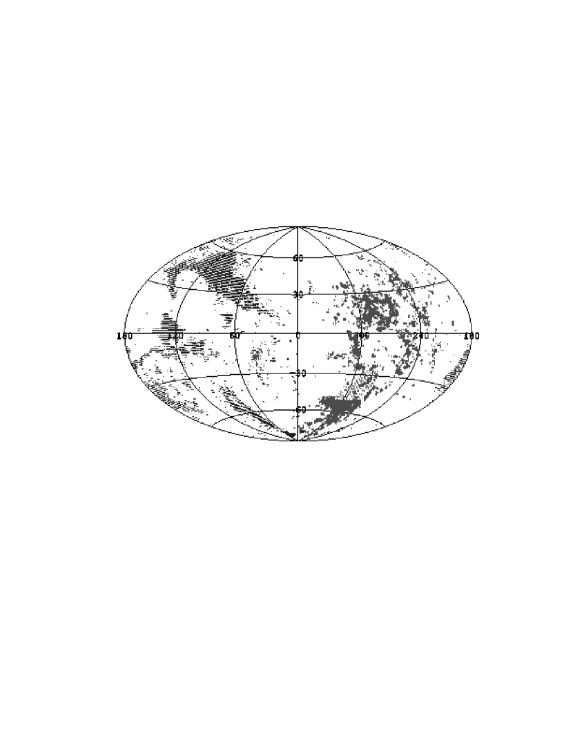
Figure 1-a: Aitoff projection of the entire sky distribution of the HVCs in Galactic coordinates, based on measurements of the 21-cm emission line of HI (adapted from Bajaja et al. bajaja (1985), Hulsbosch & Wakker hulsbosch-wakker (1988) and Morras et al. morras (2000)). Plus (or darker regions) and minus signs mark respectively the positions of the HI lines with positive and negative high velocities in the LSR frame.

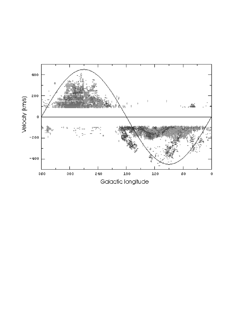
Figure 1-b: Velocity of high-velocity HI lines with respect to the LSR plotted against Galactic longitude, from the collection of data used in Fig.  1-a. The sinusoidal curve represents the $V_{\mathrm{LSR}}(\ell)$ pattern for $b=0^{\circ}$ corresponding to a hypothetical flow of HVCs, circulating in directions parallel to $\ell=90^{\circ}-270^{\circ}$.

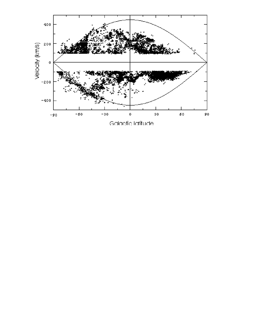
Figure 1-c: Velocity of high-velocity HI lines with respect to the LSR plotted against Galactic latitude, from the collection of data used in Fig.  1-a. The two half-cosine curves represent the $V_{\mathrm{LSR}}(b)$ pattern for $\ell=90^{\circ}$ and $270^{\circ}$ corresponding to a hypothetical flow of HVCs, circulating in directions parallel to $\ell=90^{\circ}-270^{\circ}$.

For purposes of comparison, in Figs. 2-a,  2-b and  2-c we represent the HVC distributions corresponding to a second set of data with an improvement in spatial resolution taken from Putman et al. (putman (2002)) and Giovanelli (giovanelli2 (1980)) for $\delta>-15\degr$.

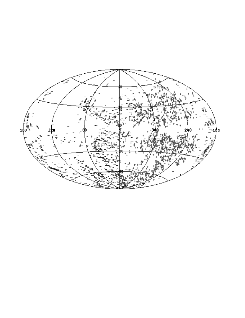
Figure 2-a: Same as Fig.  1-a, but with data adapted from Giovanelli (giovanelli (1981)) and Putman (putman (2002)). The region centered at $\ell=120^{\circ}$ and $b=30^{\circ}$ is not covered by the observations of the two surveys used here, and is left empty.

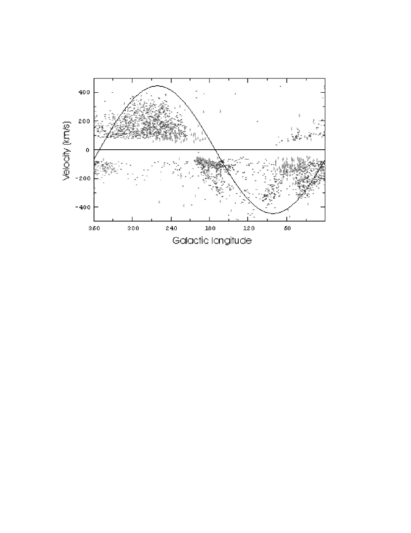
Figure 2-b: Same as Fig.  1-b, but from the collection of data used in Fig.  2-a.

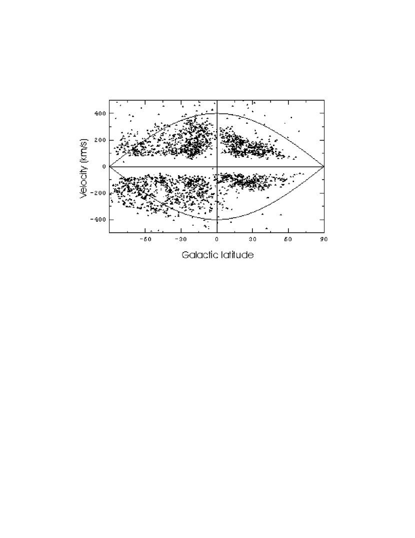
Figure 2-c: Same as Fig.  1-c, but from the collection of data used in Fig.  2-a.

The enclosing curve of the longitude-velocity distribution (Figs.  1-b and  2-b) is approximately sinusoidal and that of the latitude-velocity distribution (Figs.  1-c and  2-c) follows a cosine law. In consequence, the radial velocity distribution of the HVCs can be represented by the following formula:

$$\rho=-V\,sin(\ell)\,cos(b),$$ (1)

where $V\simeq 450\,\mathrm{km\,s^{-1}}$. This distribution law admits a simple interpretation (or “inversion”), namely: it reflects a roughly uniform flow of HVCs that comes approximately from galactic co-ordinates $\ell_{0}=90\degr$ and $b_{0}=0\degr$ and that encloses the whole Galaxy. If $V_{\sun}$ and $V_{f}$ are the velocities of the Sun and of the HVC flow with respect to the Galactic center respectively, the radial velocities of the HVCs with respect to the LSR are given by

$$\rho=-V_{\sun}\,sin(\ell)\,cos(b)-V_{f}\,cos(\ell-\ell_{0})\,cos(b-b_{0}).$$ (2)

Substituting the values of $\ell_{0}$ and $b_{0}$ into Eq. (2), we obtain Eq. (1) with $V=V_{\sun}-V_{f}$. The velocity of the HVC flow is of the order of the Solar velocity ($220\,\mathrm{km\,s^{-1}}$), and has the same direction, but its sense is reversed. In other words, the Sun is immersed in the flow of HVCs, moving counter stream. This flow of clouds seems to circulate largely in the halo or in the outskirts of the Galaxy. In the next section, we will find a clue that makes it possible to connect the flow of HVCs with the Magellanic Clouds and the Magellanic Stream.

3 Model for the origin and dynamical evolution of the high velocity clouds

In this section we will try to determinate the probable origin of the HVC flow described in Sect. 2 and the initial conditions of the phenomenon; with this we will construct a model to study the trajectories of the HVCs throughout the halo and the disk of the Galaxy. Our first objective is to show that the Magellanic Clouds have played a central role in the origin of the HVCs. For this purpose, we need to calculate the orbital plane of the Magellanic Clouds. We adopt throughout this paper a Cartesian coordinate system $(X,Y,Z)$ with the origin at the Galactic center, the X-axis pointing in the direction of the Sun’s Galactic rotation, the Y-axis pointing in the direction from the Galactic center to the Sun, and the Z-axis pointing toward the Galactic north pole. Since the Magellanic Clouds are subject to a central force due to the Galactic halo (we will ignore the forces of the galactic disk), their orbital plane can be characterized by the vector normal to this plane, namely $\@vec{N}=\@vec{r}\times\@vec{\dot{r}}$, where $\@vec{r}=(X,Y,Z)$ is the position and $\@vec{\dot{r}}=(\dot{X},\dot{Y},\dot{Z})$ is the velocity vector of the center of mass of the combined Clouds at the present epoch in the Galactocentric rest frame. We use the observational parameters of the LMC, which are better determined, as representative of the Magellanic Clouds as a whole. We adopt the following parameters for the LMC: $\ell=280\degr.5$ and $b=-32\degr.9$ for the Galactic coordinates, $50.1\,\mbox{kpc}$ for the distance from the Sun, $262.2\,\mathrm{km\,s^{-1}}$ for the heliocentric systematic velocity (van der Marel et al. marel (2002)), $\mu_{\alpha}=0.00486\arcsec\,\mathrm{yr^{-1}}$ and $\mu_{\delta}=0.00034\arcsec\,\mathrm{yr^{-1}}$ for the mean proper motion (see Table 1 of van der Marel et al. marel (2002)). To correct for the reflex motion of the Sun and to obtain the positions and velocities in the Galactocentric frame of rest, we use the IAU values $R_{\sun}=8.5\,\mbox{kpc}$ and $V_{\sun}=220\,\mathrm{km\,s^{-1}}$ and the “basic” solar motion of $16.5\,\mathrm{km\,s^{-1}}$ towards the direction of $\ell=53\degr$ and $b=25\degr$ (Allen allen (1973)). With these adopted values, we calculate the position and velocity vectors of the LMC

$$\@vec{r}_{\mathrm{LMC}}=(-41.30,1.29,-27.43)\,\mbox{kpc}$$ (3)

and

$$\@vec{\dot{r}}_{\mathrm{LMC}}=(-218,66,187)\,\mathrm{km\,s^{-1}}.$$ (4)

The resulting plane of the orbit of the LMC is represented in Fig.  3. The angle between the orbital plane and the plane perpendicular to the Galactic disk is only of the order of $10\degr$. i.e the plane of the LMC orbit is almost perpendicular to the Galactic plane. The Galactic longitude of the nodal line is nearly $82\degr$, and thus the orbital plane is almost coincident with the $X$-$Z$ plane (cf. Fig.1 of Murai & Fujimoto murai (1980)). Therefore, the three-dimensional velocity vectors representing the HVC flow described in Sect. 2 are nearly parallel to the plane of the orbit of the Magellanic Clouds. This indicates a dynamical relationship between the HVCs and the Magellanic Clouds. Our working hypothesis will be that the HVCs were ejected from the Magellanic Clouds as a result of internal processes in the Magellanic Clouds, activated likely by the collision of the LMC and SMC.

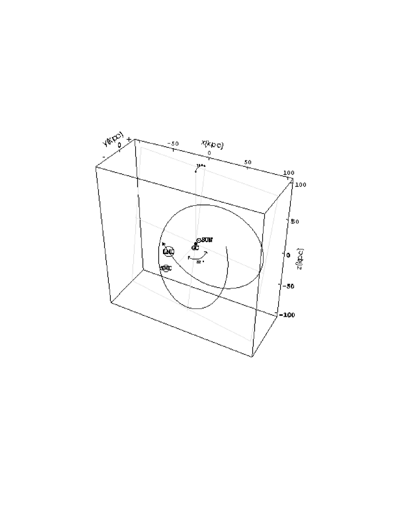
Figure 3: Locations of the LMC, the SMC and the Sun in Galactocentric coordinates $(X,Y,Z)$. The past orbit of the LMC is represented by the solid curve. The position angles of the orbital plane are indicated.

3.1 Basic equations of the model

The basic problem we should consider here is the motion of a test particle representing an HVC in the gravitational fields of the Galaxy and the Magellanic Clouds, and friction forces due to the gaseous disk of the Galaxy.

In our computations, we use the spherical gravitational potential of the halo $\psi=-V_{c}^{2}\ln r$ for the Galaxy (Murai & Fujimoto murai (1980); Lin & Lynden-Bell lin (1982)), which gives a flat rotation curve with a constant circular velocity, $V_{c}=220\,\mathrm{km\,s^{-1}}$, so that the gravitational force of the Galaxy exerted on a particle of unit mass is $-V_{c}^{2}\frac{\@vec{r}}{r^{2}}$. For the Magellanic Clouds, we use the gravitational potential of the LMC and ignore that of the SMC. We consider the SMC as another test particle (see Sect.3.2). We assume that the LMC has a Plummer-type potential with an effective radius $K=3\,\mathrm{kpc}$ (Murai & Fujimoto murai (1980)), giving a gravitational force per unit mass of $-\frac{GM_{\mathrm{LMC}}\@vec{r^{\prime}}}{(r^{\prime 2}+K^{2})^{3/2}}$, where $\@vec{r^{\prime}}(=\@vec{r}-\@vec{r}_{\mathrm{LMC}})$ denotes the position of the test particle with respect to the LMC, and $M_{\mathrm{LMC}}$ is the total mass of the LMC estimated at $0.87\times 10^{10}\,\mathrm{M}_{\sun}$ (van der Marel et al. marel (2002)).

The friction force per unit mass that acts on an HVC can be expressed as $\@vec{F}_{\mathrm{d}}=-\varepsilon\frac{nS}{m}v_{\mathrm{r}}\@vec{v}_{\mathrm{r}}$, where $\@vec{v}_{\mathrm{r}}$ is the relative velocity between the HVC and the gaseous medium in which the cloud moves, $n$ is the density of the gaseous medium at the position of the HVC, S is the head cross-section of the HVC, m is the HVC mass, and $\varepsilon$ is a dimensionless quantity $\simeq 1$. A measure of the ratio $\frac{m}{S}$ is the column density $N_{\mathrm{H}}$ of the HVC being studied, an observable quantity. We adopt a mean $N_{\mathrm{H}}$ of $7.2\times 10^{18}\,\mathrm{atoms\,cm^{-2}}$ for the HVCs. In our simplified model, the Galactic halo is empty of gas, thus $n$ depends only upon the density distribution of the gaseous disk of the Galaxy. The density $n$ may be conveniently expressed in cylindrical coordinates as $n(R,z)=\frac{\sigma(R)}{2h(R)}\exp[-\frac{\mid z\mid}{h(R)}]$, where $\sigma(R)$ and $h(R)$ are the surface density of interstellar HI and the scale height of the thickness of the HI gas layer at $R\,(=\sqrt{x^{2}+y^{2}})$, respectively. We denote by $x,y$ and $z$ the Cartesian components of the position vector $\@vec{r}$ of the test particle or HVC. From a fit of Wouterloot et al.’s (wouterloot (1990)) Table 1 we derive $\sigma(R)=1.0875\times 10^{21}\exp[-(\frac{8.24-R}{1.06\times 8.24})^{2}]\,\mathrm{atoms\,cm^{-2}}$ and $h(R)=105.8\exp[(\frac{3.37-R}{4.23\times 3.37})^{2}]\,\mathrm{pc}$ with $R$ in kpc. Assuming that the gas of the Galactic disk rotates circularly with constant velocity $V_{c}$, the velocity vector of the gaseous medium at the position of the HVC is $(\frac{V_{c}}{R}y,-\frac{V_{c}}{R}x,0)$ and hence $\@vec{v}_{\mathrm{r}}=(\dot{x}-\frac{V_{c}}{R}y,\dot{y}+\frac{V_{c}}{R}x,\dot{z})$. Under these conditions, the equations of motion of a test particle are

$$\ddot{\@vec{r}}+\frac{V_{c}^{2}\@vec{r}}{\@vec{r}^{2}}+\frac{GM_{\mathrm{LMC}}(\@vec{r}-\@vec{r}_{\mathrm{LMC}})}{(\mid\@vec{r}-\@vec{r}_{\mathrm{LMC}}\mid^{2}+K^{2})^{3/2}}-\@vec{F}_{\mathrm{d}}(\@vec{r},\dot{\@vec{r}})=0.$$ (5)

To solve this system of equations, we need first the solution of the equations of motion of the LMC in the gravitational field of the Galaxy, namely:

$$\ddot{\@vec{r}}_{\mathrm{LMC}}+\frac{V_{c}^{2}\@vec{r}_{\mathrm{LMC}}}{\@vec{r}^{2}_{\mathrm{LMC}}}=0.$$ (6)

3.2 The collision between the Large and Small Magellanic Clouds

Several authors agree that the Magellanic clouds had a close encounter (separation less than 3 kpc) between 200 and 500 Myr ago (Murai & Fujimoto murai (1980); Gardiner et al. gardiner2 (1994); Heller & Rohlfs heller (1994); Moore & Davis moore (1994); Gardiner & Noguchi gardiner (1996)). The morphological peculiarities of the Clouds such as the widely scattered distribution of HII regions around the optical bar of the LMC and the severe fragmentation of the SMC could be understood in terms of this collision.

The encounter time $t_{\mathrm{e}}$ of the Clouds is an important parameter in our model, and we want to calculate its value congruently with the other parameters adopted above. The orbit of the LMC can be computed straightforwardly by means of the numerical integration of Eq. (6) with the initial conditions given by Eqs. (3) and (4) (see Fig.  3). For simplicity we assume that the orbit of the LMC is not essentially altered by the presence of the SMC because of its lesser mass. Knowing the present position and velocity of the center of mass of the SMC, we compute the orbit of the SMC by using Eq. (5) with $\@vec{F}_{\mathrm{d}}=0$ and the solution of the orbit of the LMC. Thus we obtain the time of the closest approach of both orbits. However, the position and velocity of the SMC are not known with great precision. Therefore, in the equations we only introduce the radial component of the SMC velocity, based on the heliocentric radial velocity of $148\,\mathrm{km\,s^{-1}}$ for the SMC that was accurately measured with optical and radio-astronomical methods (Hardy et al. hardy (1989)), and leave as unknowns the proper motions and the distance, which were used for determining the tangential components of the velocity. Solving Eq. (5) with the help of Eq. (6), we obtain $\@vec{r}_{\mathrm{SMC}}$ as a function of $\mu_{\alpha}$, $\mu_{\delta}$, the distance $d$ and time $t$. By requiring that $\@vec{r}_{\mathrm{SMC}}(\mu_{\alpha},\mu_{\delta},d,t)=\@vec{r}_{\mathrm{LMC}}(t)$, we have three equations with three unknowns for each chosen past time; their solutions give us $\mu_{\alpha}(t)$, $\mu_{\delta}(t)$ and $d(t)$. Choosing the set of theoretical parameters compatible with the observational ones, we found that $\mu_{\alpha}$, $\mu_{\delta}$ and $d$ should be close to $0.00432\arcsec\,\mathrm{yr^{-1}}$, $-0.00108\arcsec\,\mathrm{yr^{-1}}$ (cf. Kroupa & Bastian kroupa (1997)) and 60.3 kpc (cf. Westerlund westerlund (1990)) respectively, and that the collision between the Clouds occurred 570 $\pm 350$ Myr ago. The uncertainty of $\pm 350$ Myr in the value of $t_{\mathrm{e}}$ was derived from that of the present velocity of the LMC (Eq. 4), $\Delta\@vec{\dot{r}}_{\mathrm{LMC}}\approx(\pm 23,\pm 36,\pm 35)\,\mathrm{km\,s^{-1}}$ (see Eq. 55 of van der Marel et al. marel (2002)), with the assumption that the rest of the adopted parameters like the distances to the Large and Small Magellanic Clouds and the gravitational potential used for the halo of the Galaxy are almost exact. The orbits of the Clouds are displayed in Figs.  4-a and  4-b.

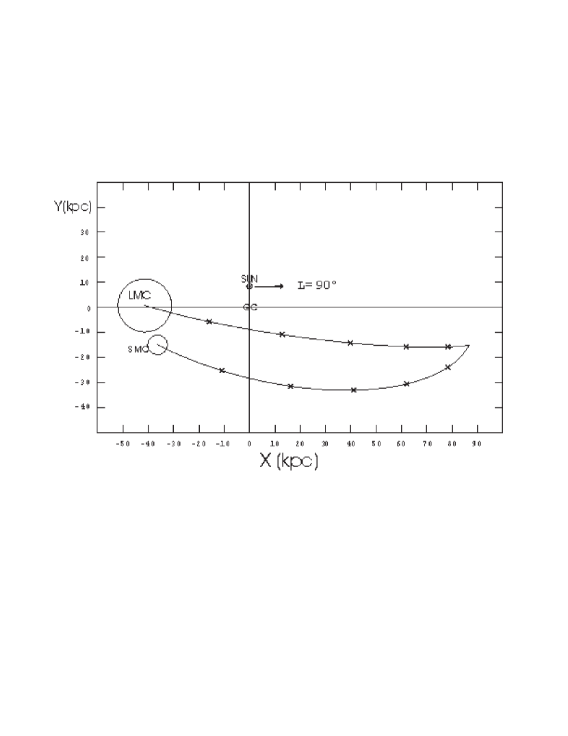
Figure 4-a: Projection of the past orbits of the LMC and the SMC on the Galactocentric $X$-$Y$ plane. The LMC and SMC positions are marked by crosses each 100 Myr.

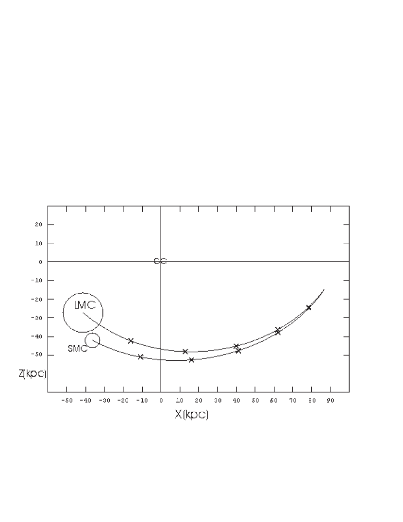
Figure 4-b: Projection of the past orbits of the LMC and the SMC on the Galactocentric $X$-$Z$ plane. The LMC and SMC positions are marked by crosses each 100 Myr.

The velocity of the LMC at the time of the collision $t_{\mathrm{e}}=-570\,\mbox{Myr}$ was

$$\@vec{\dot{r}}_{\mathrm{LMC}}(t_{\mathrm{e}})=(-100,-12,-141)\,\mathrm{km\,s^{-1}},$$ (7)

while that of the SMC was $\@vec{\dot{r}}_{\mathrm{SMC}}(t_{\mathrm{e}})=(-100,-167,-155)\,\mathrm{km\,s^{-1}}$. Thus, during the encounter, the velocity of the SMC relative to the LMC was of order $156\,\mathrm{km\,s^{-1}}$; i.e. very close to the escape velocity from the LMC ($v_{\mathrm{e}}=\sqrt{\frac{2GM_{\mathrm{LMC}}}{K}}\simeq 160\,\mathrm{km\,s^{-1}}$). To explain this, we propose that the Magellanic Clouds formed a binary system in the past and that it was broken by a sudden mass loss of the system taking place in the epoch of the collision. The collision compressed the interstellar gas of the Clouds, inducing a burst of star formation. The massive stars of this new stellar generation expelled the surrounding interstellar matter in a few millions of years at velocities greater than the escape velocity of the system, through supernova explosions and strong stellar winds. A part of the material ejected from the Clouds at that time formed the HVCs. The HVCs left likely the Magellanic Clouds as magnetized clouds of plasma (eg. Olano olano1 (1999)). Magnetic fields in HVCs have been detected by measuring Zeeman splitting of the 21-cm HI line (Kazès et. al. kazes (1991)). This magnetic self-confinement of the HVCs could explain the HVC longevity as discrete entities. This idea is coherent with the fact that the HVCs are highly ionized (Sembach et al. sembach (1999); Lehner et al. lehner (2001); Sembach et al. sembach2 (2003)). The HVCs are still generally thought of as neutral entities. However, at an early stage they were probably fully ionized. Subsequently, the evolution of their physical conditions permitted the recombination of part of the protons and electrons. On the other hand, the explanations generally given for the cloud confinement are that they are either bound by gravitationally dominant dark matter or confined by an external pressure provided by a hot gaseous Galactic halo (Espresate et al. espresate (2002); Stanimirović et al. stanimirovic (2002); Sternberg et al. sternberg (2002)).

3.3 Initial conditions of the high velocity clouds

We conjecture that the HVCs were ejected from the Magellanic Clouds as the consequence of very energetic interactions of a large number of stars born during the collision of the Clouds and the cloudy interstellar medium of the Clouds. The relevant initial conditions, namely the positions, velocities and times of the ejections of the HVCs, should therefore be characterized by distribution functions. For simplicity we assume that the HVCs were ejected from a relatively small region of the Clouds, at the central point of the collision, during a short period of time, i.e. at $t_{\mathrm{e}}=$-570 Myr. The position vector of the central point of the collision (see Sect. 3.2 and Figs.  4-a and  4-b) is then

$$\@vec{r}_{\mathrm{LMC}}(t_{\mathrm{e}})=(86.39,-15.53,-15.68)\,\mathrm{kpc},$$ (8)

and the initial position vector for all HVCs is $\@vec{r}_{0}=\@vec{r}_{\mathrm{LMC}}(t_{\mathrm{e}})$. For the initial systematic or mean velocity of the HVCs we adopt the velocity of the mass center of the LMC at the time $t_{\mathrm{e}}$, which is given by Eq. (7). The errors in Eqs. (7) and (8), i.e. in the position of the LMC in phase space at $t_{\mathrm{e}}$, are $\Delta\@vec{\dot{r}}_{\mathrm{LMC}}(t_{\mathrm{e}})\approx(\pm 3.87,\pm 0.72,\pm 1.03)\times\mid\Delta\@vec{\dot{r}}_{\mathrm{LMC}}\mid\,\mathrm{km\,s^{-1}}$ and $\Delta\@vec{r}_{\mathrm{LMC}}(t_{\mathrm{e}})\approx(\pm 0.79,\pm 0.20,\pm 1.21)\times\mid\Delta\@vec{\dot{r}}_{\mathrm{LMC}}\mid\,\mathrm{kpc}$, obtained by propagation of the errors in $\@vec{\dot{r}}_{\mathrm{LMC}}$ and $t_{\mathrm{e}}$ (Sect. 3.2).

Thus the initial total velocity of an HVC can be written as

$$\@vec{\dot{r}}_{0}=\@vec{\dot{r}}_{\mathrm{LMC}}(t_{\mathrm{e}})+\@vec{v}_{\mathrm{p}},$$ (9)

where $\@vec{v}_{\mathrm{p}}$ is the initial peculiar velocity of the HVC. The number of HVCs in the initial velocity volume $d\@vec{v}_{\mathrm{p}}$ at $\@vec{v}_{\mathrm{p}}$ is $dN=f(\@vec{v}_{\mathrm{p}})H(v_{\mathrm{p}}-v_{\mathrm{e}})d\@vec{v}_{\mathrm{p}}$ at time $t_{\mathrm{e}}$. We assume that the distribution function $f(\@vec{v}_{\mathrm{p}})$ follows Schwarzschild’s ellipsoidal law:

$$f(\@vec{v}_{\mathrm{p}})=\frac{N}{(2\pi)^{3/2}\Sigma_{1}\Sigma_{2}\Sigma_{3}}\exp{-\frac{1}{2}((\frac{\dot{x}_{\mathrm{p}}}{\Sigma_{1}})^{2}+(\frac{\dot{y}_{\mathrm{p}}}{\Sigma_{2}})^{2}+(\frac{\dot{z}_{\mathrm{p}}}{\Sigma_{3}})^{2}))},$$ (10)

where $\Sigma_{1}$, $\Sigma_{2}$ and $\Sigma_{3}$ are the three velocity dispersions in the directions of the three co-ordinate axes and $\dot{x}_{\mathrm{p}}$, $\dot{y}_{\mathrm{p}}$ and $\dot{z}_{\mathrm{p}}$ are the components of the peculiar velocity vector $\@vec{v}_{\mathrm{p}}$. The Heavyside function $H$, which is 1 for $v_{\mathrm{p}}-v_{\mathrm{e}}>0$ and 0 otherwise, takes into account that only the clouds with velocities greater than the escape velocity $v_{\mathrm{e}}$ became HVCs. In general form, the function of initial distribution of the HVCs may be written as $F(\@vec{r}_{0},\@vec{\dot{r}}_{0},t)=\delta(\@vec{r}_{0}-\@vec{r}_{\mathrm{LMC}}(t_{\mathrm{e}}))\delta(t-t_{\mathrm{e}})f(\dot{\@vec{r}}_{0}-\@vec{\dot{r}}_{\mathrm{LMC}}(t_{\mathrm{e}}))H(\dot{\@vec{r}}_{0}-\@vec{\dot{r}}_{\mathrm{LMC}}(t_{\mathrm{e}})-v_{\mathrm{e}})$, where $\delta$ is the standard delta function. The total number of HVCs (or the number of test particles used in the simulation) can be expressed by $N_{\mathrm{HVC}}=\int_{0}^{\infty}F(\@vec{r}_{0},\@vec{\dot{r}}_{0},t)d\@vec{r}_{0}d\@vec{\dot{r}}_{0}dt$, which makes it possible to determine $N$ of Eq. (10).

4 Results of the model and comparison with the observations

To reproduce the main features of the position and velocity distributions of the HVCs we calculated the orbits of about 850 test particles, which represent the HVCs. Distributing these test particles in phase space according to the distribution functions defined in Sect. 3.3, we can assign an initial position and velocity to each test particle, and calculate its present position and velocity by means of the equations of motion given in Sect. 3.1. The three dispersions of the velocity ellipsoid in Eq. (10) are the free parameters of the model. Their values can be estimated by comparing the predictions of the model with the observations. We found that the case particular of a three-dimensional Gaussian distribution is compatible with the observations, namely $\Sigma_{1}=\Sigma_{2}=\Sigma_{3}=\Sigma=120\,\mathrm{km\,s^{-1}}$. Thus, $\Sigma$ is the only free parameter of the model.

To consider the possibility of non-isotropic expulsion of material, we tried other initial ellipsoidal distributions with different values and spatial orientations of their velocity dispersions with respect to the co-ordinate axes, but none of them could produce better results than those of a Gaussian distribution. This simple distribution reproduces fairly well the kinematics and sky distributions of the Magellanic stream, the “classic” stream and the leading stream (Putman et al. 2003a ), as well as those of the rest of the HVC population. Certainly, quantitative comparisons between theoretical and observed distributions in the way developed by Saha (saha (1998)) would be desirable. However, it is beyond the scope of the present work. A proof of the robustness of our method is that the results of the simulations are rather insensitive to the uncertainties of the time of the collision, $\Delta t_{\mathrm{e}}$, and the velocity, $\Delta\@vec{\dot{r}}_{\mathrm{LMC}}(t_{\mathrm{e}})$, and position, $\Delta\@vec{r}_{\mathrm{LMC}}(t_{\mathrm{e}})$, of the centroid of the initial Gaussian distribution.

The results of the model are shown in Figs.  5-a,  5-b,  5-c,  5-d and  5-e. Comparing Fig.  5-a with Figs.  1-a and  2-a, Fig.  5-b with Figs. 1-b and  2-b, and Fig.  5-c with Figs. 1-c and  2-c, we see that the theoretical distributions are in good agreement with the corresponding observed ones. An exception is a group of HVCs that lies in a region centered at $\ell=180^{\circ}$, $b=-20^{\circ}$, whose velocities are not explained by the model. However, we should remember the simplifications and uncertainties of the observational parameters introduced into the model, as well as the probable existence of other sources of HVCs, apart from the Magellanic Clouds. Studies of HVCs in external galaxies (see Schulman et al. schulman (1996); Wakker & Woerden wakker-woerden (1997); Jiménez-Vicente & Battaner battaner (2000); Miller et. al. miller (2001)) will enable us to make a comparison with the HVC system associated with our own Galaxy and to decide the relevance of the other possible sources of HVCs, such as Galactic fountains (Bregman bregman (1980); Houck & Bregman houck (1990)). The part of the HVC population of Magellanic origin having LSR radial velocities between -100 and +100 $\mathrm{km\,s^{-1}}$ and lying at low Galactic latitudes (see Figs. 5-b and  5-c) should be indistinguishable from the interstellar clouds of the Galactic disk that are parts of supernova shells or that participate simply in the Galactic rotation.

There is a clear difference between the two Galactic hemispheres. In the northern hemisphere the population of HVCs is dominated by a few extended, complex structures (the A, C and M objects). When comparing the observed HVC distributions with the theoretical ones, we should remember this. An HVC sampled at regular angular intervals is characterized by a set of neighboring points in the ($\ell$, $b$, $\rho$) space whose number increases proportionally with the solid angle subtended by the cloud in the sky (see Sect. 2). The few northern complexes of HVCs cover a large area of the sky. Hence their densities of points in the observed distributions relative to the densities of points in the corresponding theoretical distributions should be greater than the relative densities of points corresponding to the southern HVCs. The results of our simulation agree with this picture (cf. Figs.  1-a and  5-a, and Figs  1-c and  5-c). According to our model, the explanation of these asymmetries between the northern and southern hemispheres is that in the northern Galactic hemisphere there are far fewer HVCs and they lie at much smaller distances (see Fig.  5-e). Therefore, they subtend far larger angles on the sky. The importance of the model is that it provides a probable velocity field and space distribution of the HVCs in the three dimensions (Figs. 5-d and  5-e). This information cannot be obtained from the observations so far.

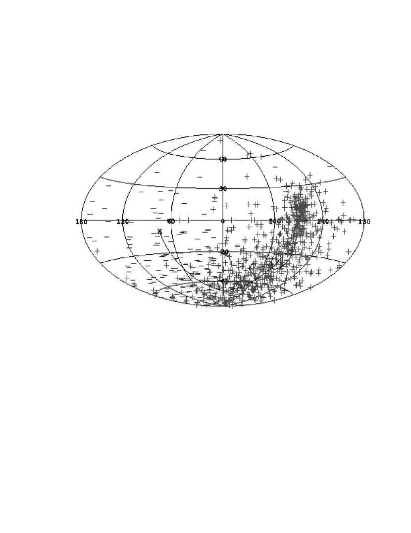
Figure 5-a: Simulated celestial distribution of the HVCs: projection of the positions of the test particles at present moment on the sky plane. The plus and minus symbols have the same meanings as in Fig.  1-a. The projections of the past orbit of the LMC (solid curve) and the present positions of the LMC and SMC (large and small projected circles) are shown. The cross at the end of the projected orbit curve is the projected position of the encounter between the LMC and the SMC. Compare this theoretical distribution with the observed ones (Figs.  1-a and  2-a).

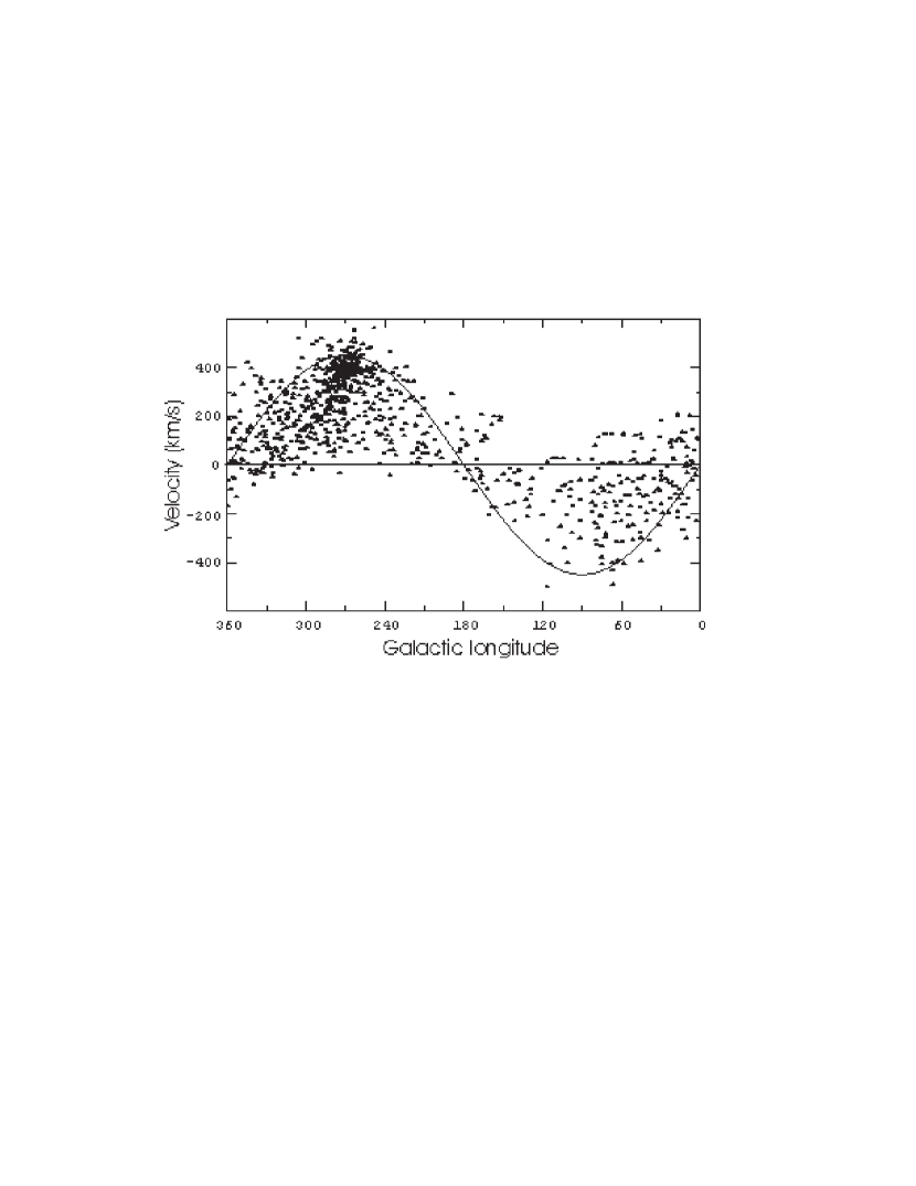
Figure 5-b: Simulated velocity-longitude relation for the HVCs: radial LSR velocities of the test particles at the present moment as a function of their respective Galactic longitudes. The solid curve has the same meaning as in Fig. 1-b. Compare this theoretical relation with the observed ones (Figs.  1-b and  2-b).

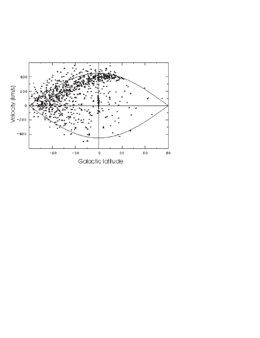
Figure 5-c: Simulated velocity-latitude relation for the HVCs: present radial LSR velocities of the test particles as a function of their respective Galactic latitudes. The solid curve has the same meaning as in Fig. 1-c. Compare this theoretical relation with the observed ones (Figs.  1-c and  2-c).

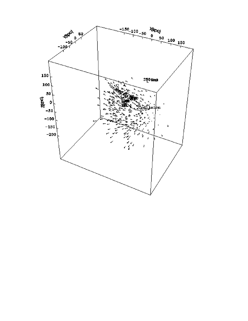
Figure 5-d: Simulated spatial distribution and velocity field in the Galactocentric rest frame for the HVCs: Present positions and velocities of the test particles. The test particles with initial velocities $\mid\@vec{v}_{\mathrm{p}}\mid<220\,\mathrm{km\,s^{-1}}$ have been omitted in the plot for clarity. The present positions of the LMC and the SMC (circles), the past orbit of the LMC (solid curve) and the point of encounter between the LMC and the SMC (circle) are represented.

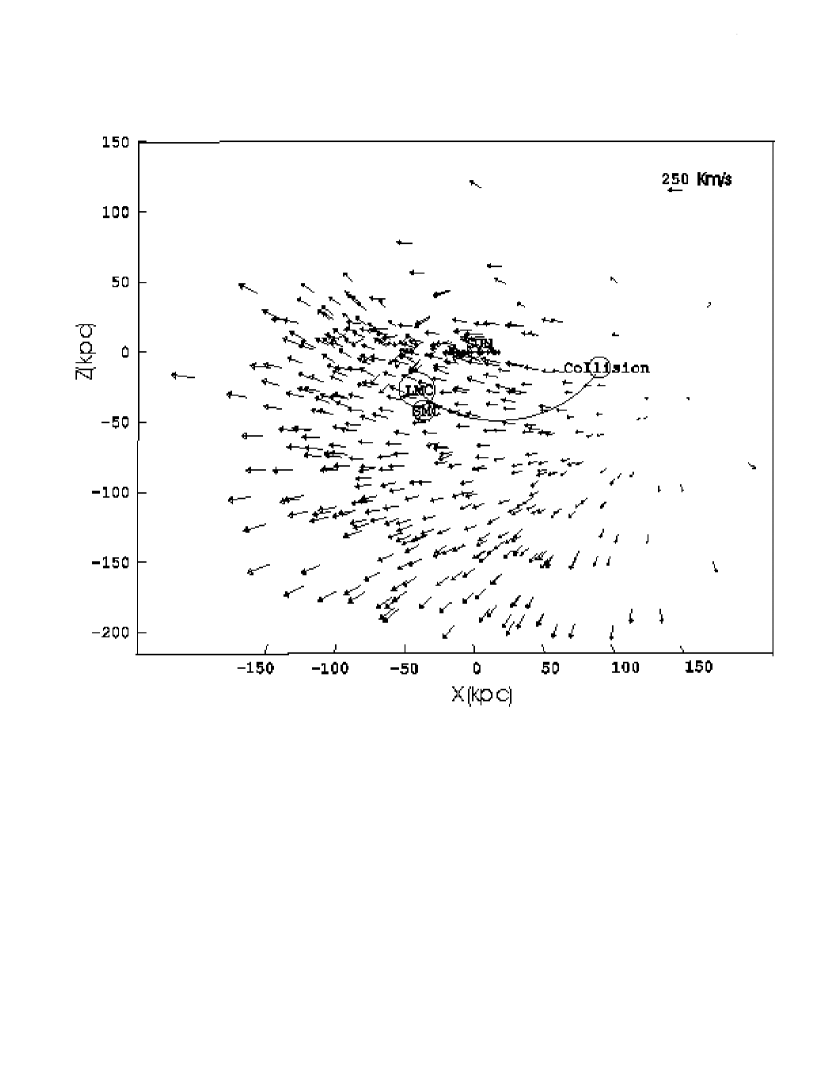
Figure 5-e: Same as Fig.  5-d, but projected on the Galactocentric $X$-$Z$ plane.

The group of HVCs spreads throughout a volume of approximately cubic 300 kpc. The mean velocity of the HVC flow is similar to that of the Magellanic Clouds, since the HVCs started their trajectories with the mean or systematic velocity of the Clouds. To illustrate this effect further, we apply the model to a set of test particles with initial peculiar velocities of the same magnitude $\mid\@vec{v}_{\mathrm{p}}\mid=$cont, but with different directions. At the present time, these test particles should form a stream that moves approximately in the same direction and sense as the Magellanic Clouds (Fig.  6-a). In addition, this cloud of particles is elongated in the direction of the velocity of rotation around the Galactic center, an effect due to the differential rotation and well known in the evolution of expanding Galactic shells (e.g. Olano olano2 (1982); Palous, Franco & Tenorio-Tagle palous (1990); Olano olano3 (2001)). Notice that the degree of concentration of the particles around the Magellanic orbit increases as the initial peculiar velocity decreases (cf. Figs.  6-a and  6-b). Also, notice that the lower the peculiar velocities of the particles, the greater the number density of particles (or HVCs), according to the initial distribution function Eq. (10). Both these effects contribute to create in the sky the appearance of the Magellanic Stream (see Fig.  5-a).

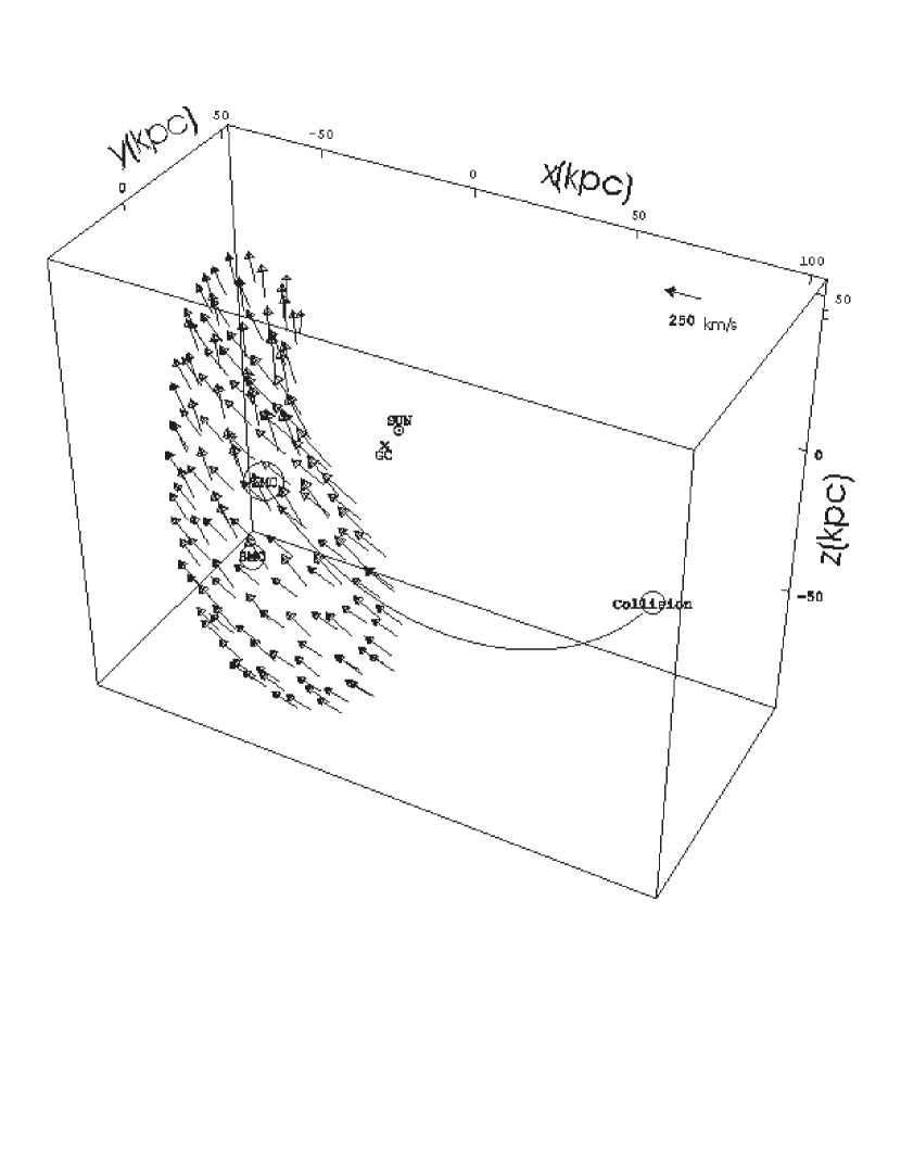
Figure 6-a: Spatial distribution and velocity field of the test particles with an initial isotropic velocity distribution characterized by $\mid\@vec{v}_{\mathrm{p}}\mid=170\,\mathrm{km\,s^{-1}}$.

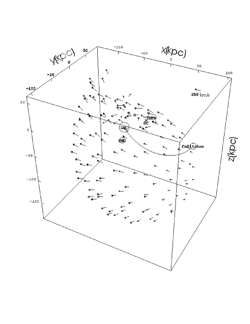
Figure 6-b: Spatial distribution and velocity field of the test particles with an initial isotropic velocity distribution characterized by $\mid\@vec{v}_{\mathrm{p}}\mid=270\,\mathrm{km\,s^{-1}}$.

From the distances to the HVCs predicted by the model and the density column data of Wakker’s (wakker-privado (2002)) list we estimated the total mass of the HVCs by means of the formula $M_{\mathrm{t}}(\mathrm{M}_{\sun})=6.085\times 10^{-19}\overline{d_{i}^{2}}(\sum_{i=1}^{N}N_{\mathrm{H}_{i}})$, where $\sum_{i=1}^{N}N_{\mathrm{H}_{i}}$ is the sum of the column densities in $\mathrm{atoms\,cm^{-2}}$ of all high-velocity profile components detected with a telescope beam of $\sim 0\degr.5$, and $\overline{d_{i}^{2}}$ is the theoretical mean squared distance of the HVCs from the Sun, expressed in $\mathrm{kpc^{2}}$. The results are $\sum_{i=1}^{N}N_{\mathrm{H}_{i}}=1.87\times 10^{23}\,\mathrm{atoms\,cm^{-2}}$ and $\sqrt{\overline{d_{i}^{2}}}=105\,\mathrm{kpc}$, hence the total HI mass of the HVCs is $\sim 1.2\times 10^{9}\mathrm{M}_{\sun}$. Assuming that the HVCs have as much ionized as neutral hydrogen (Sembach et al. sembach1 (2002)), and adopting a factor 1.3 to include $H_{\mathrm{e}}$, we obtain $M_{\mathrm{t}}=3.1\times 10^{9}\mathrm{M}_{\sun}$. Thus the Magellanic Clouds lost about 25 per cent of their original mass in the form of HVCs. This is consistent with the idea that the Clouds constituted a binary system before the last collision, whereas the important mass loss induced by this collision transformed the Clouds into an unbound system.

To study the history of the Clouds as a binary system we should calculate the relative motion of the SMC and LMC before the collision. This can be realized by means of the equation of motion resulting from the difference of Eq. (5) and Eq. (6), the boundary conditions at the moment of the collision, and a LMC mass greater than the present one (see Sect. 3.1). However, for this purpose we merely quote the pioneering study on this topic (Murai & Fujimoto murai (1980)). According to it the LMC and the SMC formed a stable binary system during $10^{10}\,\mathrm{yr}$ (see also Yoshizawa & Noguchi yoshizawa (2003)).

Another interesting result of the model is the estimate of the total energy associated with the production of the HVCs. The total initial kinetic energy of all HVCs ($\frac{1}{2}M_{\mathrm{t}}\overline{v^{2}_{\mathrm{p}}})$ is about $1.8\times 10^{57}\,\mbox{ergs}$, which implies processes that generated at least a total of $10^{58}\,\mbox{ergs}$. This huge amount of energy should have been supplied by supernovae and winds from massive stars in a starburst originated by the collision of the Clouds. The collective action of supernovae and stellar winds of a typical starburst can drive a “superwind” that may eject $10^{7}-10^{9}\,\mathrm{M}_{\sun}$ from a galaxy with a mechanical energy of $10^{57}-10^{59}\,\mbox{ergs}$ during its lifetime estimated at $10^{7}\,\mathrm{yr}$ (Heckman et al. heckman (1989)). There are various stellar generations in the Magellanic Clouds (Westerlund westerlund (1990)). There is nothing against the idea that the formation of the younger generations, with ages lower than 600 Myr, was initiated by the powerful starburst associated with the collision of the Clouds about 570 Myr ago.

5 Interaction of the high velocity clouds with the Galactic disk and generation of the Galactic warp

Most of the HVCs have not been affected by the friction force of the interstellar medium, since their orbits have not intersected with the gas layer of the Galactic disk. Here, we analyze the important group of HVCs that was strongly decelerated by the friction force of the Galactic layer and that had a strong influence on the Galactic disk.

The HVCs that penetrated the dense regions of the gaseous disk were trapped in the Galactic plane, and are participating in the Galactic rotation now (see Figs.  7-a and  7-b).

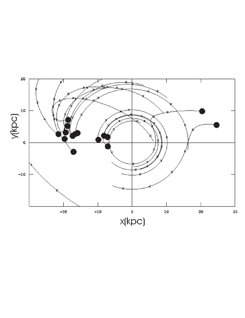
Figure 7-a: Projection, on the Galactocentric $X$-$Y$ plane, of the orbits of some of the test particles that interact with the Galactic disk. The filled circles indicate the positions of entry into the Galactic layer. The crosses mark the positions of the particle at intervals of 30 Myr. The times of entry of this subset of test particles lie between -220 and -120 Myr. The position of the Sun $(X_{\sun},Y_{\sun})$ is (0, 8.5)kpc.

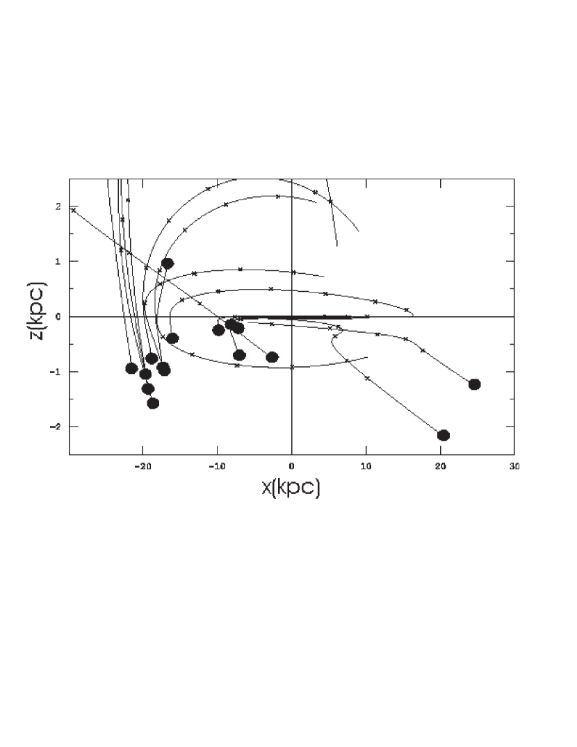
Figure 7-b: Projection of the orbits of the same test particles as those of Fig.  7-a, but on the Galactocentric $X$-$Z$ plane.

In Fig.  8, we show the positions of entry of the test particles in the gaseous layer of the Galactic disk and their present positions, resulting from the braking process. According to our model, during the last 400 Myr the Galactic disk has been profusely hit by HVCs (see Fig.  8 and Fig.  9-a).

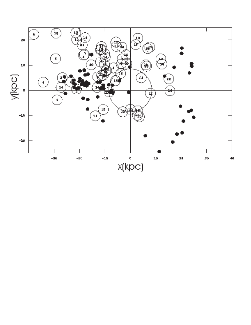
Figure 8: Same as Fig.  7-a, but for the total set of test particles that interact with the Galactic layer. The filled and open circles indicate respectively the positions of entry into the Galactic gas layer, and the present positions of the impacted regions, resulting from the interaction of the test particles with a rotating disk. We have omitted the projection of their complete orbits for clarity. The numbers inside the circles refer to the ages of impacted regions in units of 10 Myr, defining age as the time elapsed from the entry of the particle into the Galactic layer up to the present. The solar circle is indicated.

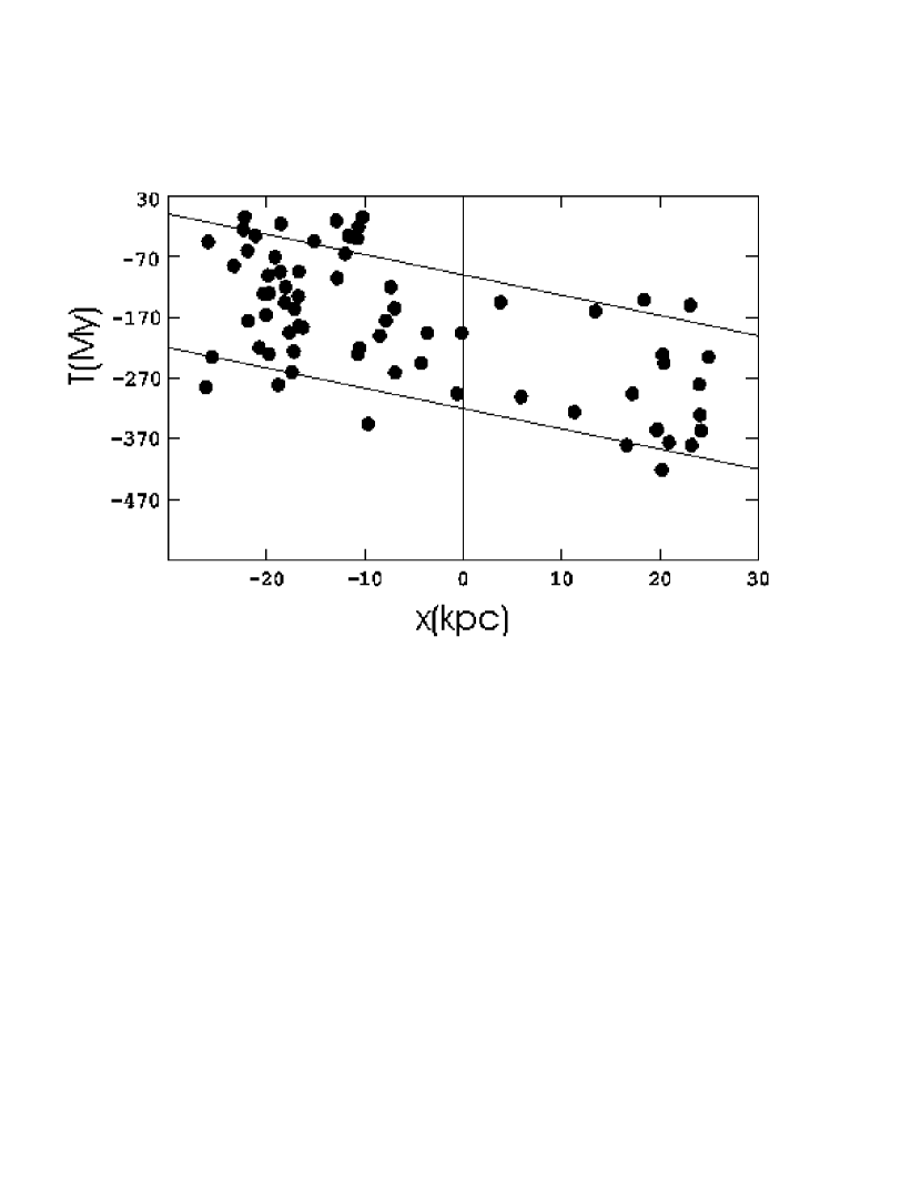
Figure 9-a: Correlation between the times of entry of the test particles into the Galactic layer and the positions of the particles projected on the $X$-axis. The solid lines represent the position of the front edge (lower line) and the back edge of the accretion front as a function of time. Negative time means before the present.

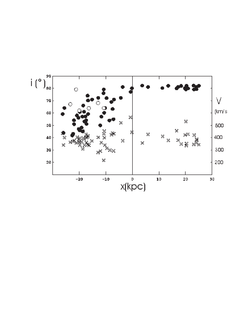
Figure 9-b: Angles (filled and open circles) and velocities (crosses) of entry of the test particles into the Galactic layer versus the respective positions projected on the $X$-axis. The open circles refer to angles of entry from above the Galactic plane.

The detailed description of the interaction of HVCs with the Galactic disk is beyond the scope of the present study. Tenorio-Tagle (tenorioa (1980), tenoriob (1981)) analyzed the physics of the collisions of HVCs with the Galactic disk. It is clear that the impact of HVCs upon the Galactic disk should be an important source for producing shells and supershells. This mechanism of creation of large-scale structures in the interstellar medium can account for many of the observational details of the large HI shells lying beyond the solar circle (Mirabel mirabelb (1982); Heiles heiles (1984)). In connection with this, it is interesting to compare the theoretical distribution of the impacts of test particles on the Galactic disk (Fig. 8), with the location of observed shells and supershells of HI (McClure-Griffiths et al. mcclure (2002)). Evidence for interactions of HVCs with the gas in the Galactic plane was found by several authors (see Tripp et al. tripp (2003) and the reviews of Tenorio-Tagle & Bodenheimer tenorio-bodenheimer (1988) and Pöppel poeppel (1997)).

In the next paragraphs of this section we will show that the flow of HVCs onto the Galactic disk over a period of 400 Myr has caused a major disturbance in the Galaxy. As a consequence of the fall of clouds, a burst of star formation involving the whole Galactic disk should have started 400 Myr ago and is still going on (Barry barry (1988); Noh & Scalo noh (1990)). There are observational details of the vertical structure of the Galactic disk, such as peculiar departures from the midplane or huge depressions delineated by young star-gas supercomplexes (Alfaro et al. alfaro (1991)), that may be explained in terms of HVC-disk collisions that induced star formation (Cabrera-Ca$\tilde{\rm n}$o et al. cabrera (1995)). Further predictions provided by our model are the times, velocities and angles of entry of the HVCs in the Galactic layer (see Figs.  9-a and  9-b). The angle of entry (or incidence) of an HVC is defined as the angle of the direction of motion of an HVC with respect to the vertical ($Z$-axis). The angle of entry is an important parameter for the hydrodynamic simulations of the collision process (Comerón & Torra comeron (1991); Franco et al. franco (1988)). The times, velocities and angles of entry correspond to the point at which the friction coefficient reaches the threshold value $\varepsilon\frac{nS}{m}=10^{-5}\,\mathrm{pc^{-1}}$ (see Sect. 3.1). Figs  9-a and  9-b show interesting differences between the times and angles of entry on the right side of the Galactic disk (positive $X$-axis) and those on the left side. The HVCs arrived first at the right side of the Galactic disk, while there was a delay of $\sim 150\,\mathrm{Myr}$ for those arriving at the left side of the disk. On the right side of the disk the HVCs impinged on the disk from below with angles of entry $\sim 80\degr$, i.e. almost a grazing incidence. In contrast, on the left side of disk the angles of entry are lower; and although most of the HVCs entered from below too, there were some HVCs that entered from above.

In the following we examine whether there is a causal relationship between the HVC-disk interaction and the generation of the Galactic warp. Galactic warps are very complex phenomena (see López-Corredoira et al. lopez (2002), García-Ruiz et al. garcia (2002) and references therein). We will analyze only a few aspects of the problem in the light of our model. During the last 450 Myr, the flow of HVCs has been exerting a pressure on the gaseous disk which could have caused the distortion of the disk of the Galaxy. Since about 7 per cent of the test particles of the simulation impacts within the galactocentric radius $R=$ 25 kpc, the mass in the form of HVCs accumulated by the disk is $0.07\times M_{\mathrm{t}}\sim 2.2\,10^{8}\,\mathrm{M}_{\sun}$. Therefore, the rate of mass accretion per surface unit is $\gamma=600\,\mathrm{M}_{\sun}\,\mathrm{kpc^{-2}\,Myr^{-1}}$, taking into account that the time during which the flow acted on the disk at a fixed point in the $(X,Y,Z)$ frame was nearly 200 Myr (see Fig. 9-a). Let us consider a cylinder of unit cross-section with generators parallel to the $Z$-axis and height $h(R)$ as a volume element of the gaseous disk of the Galaxy at $R$. The accretion process acting on the volume element generates a force in $Z$ per unit of mass that can be written as $F_{z}=\frac{\gamma}{\sigma(R)}\overline{v}cos(\overline{i})$, where $\overline{v}$, $\overline{i}$ are the mean velocity and angle of entry, and $\sigma(R)$ is the surface density of the gaseous disk at $R$ (see Sect. 3.1).

To describe the gas motion of the volume element under the effects of the additional force associated with the mass accretion, we use cylindrical coordinates, $(R,\theta,Z)$, representing the galactocentric radius, azimuth and vertical distance from the plane $b=0\degr$ of the mass center of the chosen volume element. The gas motion in the $Z$-direction is governed by the force $F_{z}$ and the restoring force of the stellar disk $F=-\lambda^{2}Z$. It can be expressed by

$$Z(t)=Z_{0}(t_{\mathrm{e}})+\frac{sin(\lambda(t-t_{\mathrm{e}}))}{\lambda}\int_{0}^{t-t_{\mathrm{e}}}F_{z}cos(\lambda\tau)d\tau-\frac{cos(\lambda(t-t_{\mathrm{e}}))}{\lambda}\int_{0}^{t-t_{\mathrm{e}}}F_{z}sin(\lambda\tau)d\tau$$ (11)

, (see Eq. 5.713 of Chandrasekhar chandrasekhar (1943)). As initial conditions of the disk in $Z$ we put $Z_{0}=\dot{Z}_{0}=0$ at the time origin $t_{\mathrm{e}}=-570\,\mbox{Myr}$. Ignoring the effects of the $(X,Y)$ component of the force associated with the mass accretion, and assuming circular rotation, we have $\theta(t)=\theta_{0}(t_{\mathrm{e}})+\frac{V_{c}}{R}(t-t_{\mathrm{e}})$.

The flow of HVCs moves parallel to the $X$-axis. Therefore, we can think of the interaction of the HVCs with the disk as an accretion front perpendicular to the $X$-axis, propagating in the $X$ direction with a constant velocity $v_{\mathrm{a}}$. Then the position of the accretion front as a function of time is $X_{\mathrm{a}}(t)=v_{\mathrm{a}}t+X_{0}(t_{\mathrm{e}})$ (see Fig. 9-a). The volume element enters the front when $X=R\,sin(\theta(t))=X(t)_{\mathrm{a}}$, a condition that allows us to determine the entry time $t_{1}$. The time at which the volume element leaves the rear zone of the accretion front, $t_{2}$, is determined by solving $X=X(t)_{\mathrm{a}}+\Delta X_{\mathrm{a}}$ for t, where $\Delta X_{\mathrm{a}}$ is the thickness of the accretion front. The times $t_{1}$ and $t_{2}$ and the duration of the process of mass accretion, $t_{\mathrm{a}}=t_{2}-t_{1}$, depend on $\theta$ and $R$ of the volume element (see Fig.  10-a). At large galactocentric radii the time intervals of mass accretion $t_{\mathrm{a}}$ in regions of the third and fourth Galactic quadrants are longer than those in the first and second quadrants, i.e the outer regions in the third and fourth Galactic quadrants are the most affected by the interaction with the HVCs. For each volume element, the force $F_{z}$ acts between the corresponding times $t_{1}$ and $t_{2}$, vanishing outside this time interval. Hence, Eq. (11) becomes $Z(\theta,R,t)=\frac{F_{z}}{\lambda^{2}}(cos\lambda(t_{2}+t_{\mathrm{e}}-t)-cos\lambda(t_{1}+t_{\mathrm{e}}-t))$. This is a general expression for the $Z$ deformation of the Galactic layer due to the flow of HVCs. At t=0 this equation can reproduce roughly the present configuration of the Galactic warp, if the period of vertical oscillation $\frac{1}{2\pi\lambda}\sim 450\,\mathrm{Myr}$ (see Fig.  10-b). This value seems reasonable, because at large galactocentric radii the restoring force should be small. Note that the model can explain the overall pattern of positive vertical displacements in the first and second Galactic quadrants, as well as the less pronounced displacements toward negative $Z$ in the third and fourth quadrants (cf. our Fig. 10-b with Figs. 57b and 60b of Burton burton (1991)).

The first explanation proposed for the Galactic warp was that the Galaxy is passing through a continuous intergalactic medium (Kahn & Woltjer kahn (1959)). In contrast, we propose an interaction of the Galactic disk with a transient circumgalactic flow of HVCs produced by a single event of mass transfer from the Magellanic Clouds. Our model shows that the flow of HVCs is able to produce the formation of the Galactic warp. Future extensions of the model should contemplate consequences of the process of mass accretion such as large deviations from the circular rotation of the gaseous disk and the sudden increment of the rate of star formation and of the input of energy in the interstellar medium. The HVCs have injected energy at a rate of $\sim 10^{50}\,\mathrm{ergs\,kpc^{-2}\,Myr^{-1}}$ into the Galactic disk during the last 400 Myr. A question we should address, among others, should be the role played by this important source of energy in the production and maintenance of the diverse phases of the interstellar medium (Kulkarni & Heiles kulkarni (1988); Elmegreen elmegreen (1991); Heiles & Troland heiles-troland (2003)). Another interesting question is whether there exists any genetic or dynamic link between the Galactic warp and a ring of stars in the plane of the Galaxy, at a Galactocentric radius of 18-20 kpc, which may completely encircle the Galaxy (Ibata et al. ibata (2003); Yanny et al. yanny (2003)).

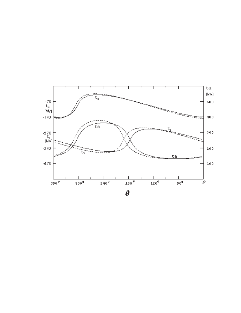
Figure 10-a: The time $t_{1}$ at which the head of the accretion front crosses a disk region, and the time $t_{2}$ at which the back of the accretion front leaves the region, as a function of the present azimuth for the regions at $R=$ 22 kpc (dashed line) and $R=$ 24 kpc (solid line). The duration of the transit of the accretion front, $t_{\mathrm{a}}=t_{2}-t_{1}$, is also represented as a function of the present azimuth.

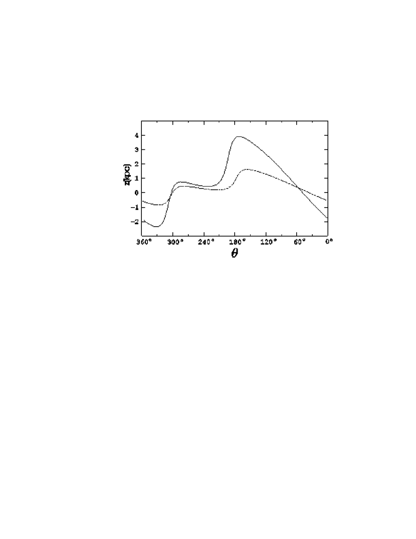
Figure 10-b: Vertical $Z-$distances of the midplane of the Galactic layer from the plane $b=0$ at the Galactocentric distances $R=$ 22 kpc (dashed line) and $R=$ 24 kpc (solid line) as a function of the azimuth of the region, according to the simulation of the interaction between the accretion front due to the flow of HVCs and the Galactic gas layer.

6 Conclusions

We have shown that the majority of the HVCs have a common origin linked to the dynamic evolution of the Magellanic Clouds. During a long time these two small satellite galaxies have likely behaved as a binary system under the effects of the tidal perturbations of the Galaxy. The two Clouds have probably approached each other several times in the past, until the Clouds collided catastrophically about 570 Myr ago. We assumed that the collision triggered a burst of stellar formation in the Clouds. The superwind driven by the starburst blew the HVCs as magnetized clouds into the massive halo of the Galaxy. As a consequence, the Milky Way is likely surrounded by a mist of highly ionized gas at high velocity, the HVCs being the denser concentrations.

The catastrophic loss of matter was of a significant amount. Probably it permitted the SMC to reach escape velocity, disrupting the binary system. According to the results of our model the amounts of matter and mechanical energy liberated in the form of HVCs were of the order of $3.1\times 10^{9}\,\mathrm{M}_{\sun}$ and $1.8\times 10^{57}\,\mathrm{ergs}$, respectively. In the numerical simulation of the process, we assumed that the HVCs were ejected from the Clouds 570 Myr ago in all directions with peculiar velocities larger than the escape velocity of $160\,\mathrm{km\,s^{-1}}$, and following a Gaussian distribution law. Because of these initial expansion velocities, the cloud of HVCs, or metacloud, expanded from the center of collision of the Magellanic Clouds, reaching its present size of $\sim 300\,\mbox{kpc}$, and filling a great part of the halo volume of the Galaxy. As the initial mean velocity of the HVCs was that of the Clouds at the time of the ejections of HVCs, the centroid of the group of HVCs (metacloud) describes an orbit close to the orbit of the Magellanic Clouds (i.e. approximately in the direction $\ell=90\degr-270\degr$). To an observer at the position of the Sun, this gives the impression of a flow of HVCs coming from $\ell=90\degr$. As a consequence of the initial velocity distribution of the HVCs, a larger number of HVCs tended to concentrate towards the Magellanic orbit behind the present position of the Clouds, whereas other HVCs moved ahead of them, forming the Magellanic Stream.

The passage of the HVC flow through the Galactic disk had transcendent consequences for the evolution of the gaseous layer of the Galaxy. The outer gas layer of the Galaxy was considerably displaced in the $Z$-direction from its equilibrium position. The Galactic disk accumulated mass coming in the form of HVCs at an average rate of $600\,\mathrm{M}_{\sun}\,\mathrm{kpc^{-2}\,Myr^{-1}}$ over a period of 200 Myr. Due to the time dependence of the mass accretion upon the azimuth of the region, the effects on the first and second Galactic quadrants at large galactocentric radii were different from those on the third and fourth ones. These are perhaps some of the clues to understand the genesis of the Galactic warp. The collisions of the HVCs with the Galactic disk might have exerted notable influences on the large-scale morphology and energy of the interstellar medium.

- (1) Allen, C. W. 1973, Astrophysical Quantities, 3rd ed., Athlone Press, London.
- (2) Alfaro, E. J., Cabrera-Cao, J., & Delgado, A. J. 1991, ApJ, 378, 106
- (3) Bajaja, E., Cappa de Nicolau, C. E., Cersósimo, J. C., Loiseau, N., Martín, M. C., Morras, R., Olano, C. A., & Pöppel, W. G. L. 1985, ApJS, 58, 143
- (4) Bajaja, E., Morras, R., & Pöppel, W. G. L. 1987, Publ. Astron. Inst. Czech. Ac. Sci., 69, 237
- (5) Barry, D. C. 1988, ApJ, 334, 436
- (6) Blitz, L., Spergel, D. N., Teuben, P. J., Hartmann, D., & Burton, W. B. 1999, ApJ, 514, 818
- (7) Braun, R., & Burton, W. B. 2000, A&A, 354, 853
- (8) Bregman, J. N. 1980, ApJ, 236, 577
- (9) Burton, W. B. 1991, in Saas-Fee Advanced Course 21, The Galactic Interstellar Medium, ed. D. Pfenniger & P. Bartholdi (New York: Springer-Verlag), 1
- (10) Cabrera-Cao, J., Moreno, E., Franco, J., & Alfaro, E. J. 1995, ApJ, 448, 149
- (11) Chandrasekhar, S. 1943, Principles of Stellar Dynamics, Dover Publications, Inc, New York.
- (12) Comerón, F., & Torra, J. 1991, A&A, 241, 57
- (13) Craig, I. J. D., & Brown, J. C. 1986, Inverse Problems in Astronomy, Adam Higer Ltd, Bristol & Boston.
- (14) Elmegreen, B. G. 1991, in Saas-Fee Advanced Course 21, The Galactic Interstellar Medium, ed. D. Pfenniger & P. Bartholdi (New York: Springer-Verlag), 157
- (15) Espresate, J., Cantó, J., & Franco, J. 2002, ApJ, 575, 194
- (16) Franco, J., Tenorio-Tagle, G., Bodenheimer, P., Różycska, M., & Mirabel, I. F. 1988, ApJ, 333, 826
- (17) García-Ruiz, I., Kuijken, K., & Dubinski, J. 2002, MNRAS, 337, 459
- (18) Gardiner, L. T., & Noguchi, M. 1996, MNRAS, 278, 191
- (19) Gardiner, L. T., Sawa, T., & Fujimoto, M. 1994, MNRAS, 266, 567
- (20) Giovanelli, R. 1980, AJ, 85, 1155
- (21) Giovanelli, R. 1981, AJ, 86, 1468
- (22) Hardy, E., Suntzeff, N. B., & Azzopardi, M. 1989, ApJ, 344, 210
- (23) Heckman, T. M., Armus, L., & Miley, G. K. 1990, ApJS, 74, 833
- (24) de Heij, V., Braun, R., & Burton, W. B. 2002a, A&A, 391, 67
- (25) de Heij, V., Braun, R., & Burton, W. B. 2002b, A&A, 392, 417
- (26) Heiles, C. 1984, ApJS, 55, 585
- (27) Heiles, C., & Troland, T. H. 2003, ApJ, 586, 1067
- (28) Heller, P., & Rohlfs, K. 1994, A&A, 291, 743
- (29) Houck, J. C., & Bregman, J. N. 1990, ApJ, 352, 506
- (30) Hulsbosch, A. N. M., & Oort, J. H. 1973, A&A, 22, L153
- (31) Hulsbosch, A. N. M., & Wakker, B. P. 1988, A&AS, 75, 191
- (32) Ibata, R. A., Irwin, M. J., Lewis, G. F., Ferguson, A. M. N., & Tanvir, N. 2003, MNRAS, 340, L21
- (33) Jiménez-Vicente, J., & Battaner, E. 2000, A&A, 358, 812
- (34) Kahn, F. D., & Woltjer, L. 1959, ApJ, 130, 705
- (35) Kazès, I., Troland, T. H., & Crutcher, R. M. 1991, A&A, 245, L17
- (36) Kerr, F. J., & Sullivan III, W. T. 1969, ApJ, 158, 115
- (37) Kroupa, P., & Bastian, U. 1997, New Astronomy, 2, 77
- (38) Kulkarni, S. R, & Heiles, C. 1988, in Galactic and Extragalactic Radio Astronomy, ed. G. L. Verschuur & K. I. Kellerman (New York: Springer), 95
- (39) Lehner, N., Keenan, F. P., & Sembach, K. R. 2001, MNRAS, 323, 904
- (40) Lin, D. N. C., & Lynden-Bell, D. 1982, MNRAS, 198, 707
- (41) Lockman, F. J., Murphy, E. M., Petty-Powell, S., & Urick, V. J. 2002, ApJS, 140, 331
- (42) López-Corredoira, M., Betancort-Rijo, J., & Beckman, J. E. 2002, A&A, 386, 169
- (43) Maloney, P. R., & Putman, M. E. 2003, ApJ, 589, 270
- (44) McClure-Griffiths, N. M., Dickey, J. M., Gaensler, B. M., & Green, A. J. 2002, ApJ, 578, 176
- (45) Merritt, D. 1996, AJ, 112, 1085
- (46) Miller, E. D., Bregman, J. N., & Wakker, B. P. 2001, Gas and Galaxy Evolution, ASP Conference Proceeding, 224, 533
- (47) Mirabel, I. F. 1981, ApJ, 250, 528
- (48) Mirabel, I. F. 1982, ApJ, 256, 112
- (49) Moore, B., & Davis, M. 1994, MNRAS, 270, 209
- (50) Morras, R., Bajaja, E., Arnal, E. M., & Pöppel, W. G. L. 2000, A&AS, 142, 25
- (51) Murai, T., & Fujimoto, M. 1980, PASJ, 32, 581
- (52) Noh, H-R., & Scalo, J. 1990, ApJ, 352, 605
- (53) Olano, C. A. 1982, A&A, 112, 195
- (54) Olano, C. A. 1999, Ap&SS, 266, 347
- (55) Olano, C. A. 2001, AJ, 121, 295
- (56) Oort, J. H. 1966, Bull. Astron. Inst. Netherlands, 18, 421
- (57) Oort, J. H. 1969, Nat, 224, 1158
- (58) Oort, J. H. 1970, A&A, 7, 381
- (59) Palous, J., Franco, J., & Tenorio-Tagle, G. 1990, A&A, 227, 175
- (60) Pöppel, W. G. L. 1997, Fund. Cosm. Phys., 18, 1
- (61) Putman, M. E. et al. 2002, AJ, 123, 873
- (62) Putman, M. E. et al. 2003a, ApJ, 586, 170
- (63) Putman, M. E. et al. 2003b, ApJ, 597, 948
- (64) Quilis, V., & Moore, B. 2001, ApJ, 555, L95
- (65) Richter, P., Sembach, K. R., Wakker, B. P., & Savage, B. D. 2001, ApJ, 562, L181
- (66) Saha, P. 1998, AJ, 115, 1206
- (67) Schulman, E., Bregman, J. N., Brinks, E., & Roberts, M. S. 1996, AJ, 112, 960
- (68) Sembach, K. R., et al. 2003, ApJS, 146, 165
- (69) Sembach, K. R., Gibson, B. K., Fenner, Y., & Putman, M. E. 2002, ApJ, 572, 178
- (70) Sembach, K. R., Savage, B. D., Lu, L., & Murphy, E. M. 1999, ApJ, 515, 108
- (71) Stanimirović, S., Dickey, J. M., Krc̆o, M., & Brooks, A. M. 2002, ApJ, 576, 773
- (72) Sternberg, A., McKee, C. F., & Wolfire, M. G. 2002, ApJS, 143, 419
- (73) Tenorio-Tagle, G. 1980, A&A, 88, 61
- (74) Tenorio-Tagle, G. 1981, A&A, 94, 338
- (75) Tenorio-Tagle, G., & Bodenheimer, P. 1988, ARA&A, 26, 145
- (76) Tripp, T. M. et al. 2003, AJ, 125, 3122
- (77) Tufte, S. L., Reynolds, R. J., & Haffner, L. M. 1998, ApJ, 504, 773
- (78) van der Marel, R. P, Alves, D. R., Hardy, E., & Suntzeff, N. B. 2002, AJ, 124, 2639
- (79) Verschuur, G. L. 1993, ApJ, 409, 205
- (80) Wakker, B. P. 2001, ApJS, 136, 463
- (81) Wakker, B. P. 2002, private communication.
- (82) Wakker, B. P., & van Woerden, H. 1997, ARA&A, 35, 217
- (83) Westerlund, B. E. 1990, A&A Rev., 2, 29
- (84) Wouterloot, J. G. A., Brand, J., Burton, W. B., & Kwee, K. K. 1990, A&A, 230, 21
- (85) Yanny, B. et al. 2003, ApJ, 588, 824
- (86) Yoshizawa, A. M., & Noguchi, M. 2003, MNRAS, 339, 1135