Polarized Cosmological Gravitational Waves from Primordial Helical Turbulence

Abstract

We show that helical turbulence produced during a first-order phase transition generates circularly polarized cosmological gravitational waves (GWs). The characteristic frequency of these GWs for an extreme case of the phase transition model is around $10^{-3}$ — $10^{-2}$ Hz with an energy density parameter as high as $10^{-12}$ — $10^{-11}$. The possibility of detection is briefly discussed.

Since cosmological GWs propagate without significant interaction after they are produced, once detected they should provide a powerful tool for studying the early Universe at the time of GW generation tasi . Various mechanisms for cosmological GW generation have been studied, including: quantum fluctuations during inflation inflation ; bubble wall motion and collisions during phase transitions kos ; cosmological magnetic fields magnet ; kmk02 ; and plasma turbulence kmk02 ; dolgov ; nic .

In this letter we focus on polarization of cosmological GWs generated by helical stochastic turbulent motions helicity ; helicity2 ; kr05 . We find that helical turbulence generates circularly polarized stochastic GWs and we compute the polarization degree. The formalism we use is general and can be applied to study the generation of stochastic GWs by any helical vector field (e.g., helical magnetic fields cdk04 ; kr05 ). Primordial polarized GWs might be generated from quantum fluctuations accounting for the gravitational Chern-Simons term rodriguez .

GWs are sourced by the transverse and traceless part of the stress-energy tensor $T_{\mu\nu}$ mtw73 . In the case at hand $T_{\mu\nu}$ describes a turbulent cosmological fluid after a phase transition kos ; kmk02 ; dolgov . For spatial indices $i\neq j$, $T_{ij}({\bf x})=(p+\rho)u_{i}({\bf x})u_{j}({\bf x})$, where $p$ and $\rho$ are the fluid pressure and energy density and ${\mathbf{u}}({\mathbf{x}})$ is the fluid velocity. The fluid enthalpy density $p+\rho$ is taken to be constant throughout space. The transverse and traceless part of $T_{ij}$ in Fourier space is $\Pi_{ij}({\mathbf{k}})=[P_{il}({\mathbf{\hat{k}}})P_{jm}({\mathbf{\hat{k}}})-\frac{1}{2}P_{ij}({\mathbf{\hat{k}}})P_{lm}({\mathbf{\hat{k}}})]T_{lm}({\mathbf{k}})$, where $P_{ij}({\mathbf{\hat{k}}})=\delta_{ij}-{\hat{k}}_{i}{\hat{k}}_{j}$ with ${\hat{k}}_{i}=k_{i}/k$. Consistent with observations we have assumed flat space sections.

To model the turbulence we assume that in the early Universe at time $t_{\rm{in}}$ (at a phase transition) liberated vacuum energy $\rho_{\rm{vac}}$ is converted into (turbulent) kinetic energy of the cosmological plasma with an efficiency $\kappa$ over a time scale $\tau_{\rm{stir}}$ on a characteristic source length scale $L_{S}$ kos . After generation, the turbulence kinetic energy cascades from larger to smaller scales. The cascade stops at a damping scale, $L_{D}$, where the turbulence energy is removed by dissipation. As usual, we assume that the turbulence is produced in a time much less than the Hubble time, $\tau_{\rm{stir}}\ll 1/H_{\rm{in}}$ — here $H_{\rm{in}}$ is the Hubble parameter at $t_{\rm{in}}$ — kmk02 ; dolgov , and therefore we ignore the expansion of the Universe when studying the generation of GWs. In this case the GW equation of motion, in wave number space, is mtw73

$${\ddot{h}}_{ij}({\mathbf{k}},t)+k^{2}h_{ij}({\mathbf{k}},t)=16\pi G\Pi_{ij}({\mathbf{k}},t).$$ (1)

Here $G$ is the Newtonian gravitational constant, and $h_{ij}({\mathbf{k}})=\int d^{3}\!x\,e^{i{\mathbf{k}}\cdot{\mathbf{x}}}h_{ij}({\mathbf{x}})$ and $h_{ij}({\mathbf{x}})=\int d^{3}\!k\,e^{-i{\mathbf{k}}\cdot{\mathbf{x}}}h_{ij}({\mathbf{k}})/(2\pi)^{3}$ is the Fourier transform pair of the tensor metric perturbation which is defined $h_{ij}=\delta g_{ij}$ ($h_{ii}=0$ and $h_{ij}{\hat{k}}^{j}=0$). We use natural units $\hbar=1=c$, physical/proper wave numbers (not comoving ones), and an overdot denotes a derivative with respect to time $t$.

Stochastic turbulent fluctuations generate stochastic GWs. Gaussian-distributed GWs may be characterized by the wave number-space two-point function

$$\langle h^{\star}_{ij}({\mathbf{k}},t)h_{lm}({\mathbf{k}^{\prime}},t)\rangle~{}~{}~{}~{}~{}~{}~{}~{}~{}~{}~{}~{}~{}~{}~{}~{}~{}~{}~{}~{}~{}~{}~{}~{}~{}~{}~{}~{}~{}~{}~{}~{}~{}~{}~{}~{}~{}~{}~{}~{}~{}~{}$$

$$=(2\pi)^{3}\delta^{(3)}({\bf k}-{\bf k^{\prime}})\left[{\mathcal{M}}_{ijlm}H(k,t)+i{\mathcal{A}}_{ijlm}{\mathcal{H}}(k,t)\right].~{}$$ (2)

Here $H({k},t)$ and ${\mathcal{H}}({k},t)$ characterize the GW amplitude and polarization, $4{\mathcal{M}}_{ijlm}({\mathbf{\hat{k}}})\equiv P_{il}P_{jm}+P_{im}P_{jl}-P_{ij}P_{lm}$, and $8{\mathcal{A}}_{ijlm}({\mathbf{\hat{k}}})\equiv{\hat{\bf k}}_{q}(P_{jm}\epsilon_{ilq}+P_{il}\epsilon_{jmq}+P_{im}\epsilon_{jlq}+P_{jl}\epsilon_{imq})$ are tensors, and $\epsilon_{ijl}$ is the fully antisymmetric symbol. Choosing the coordinate system so that unit vector ${\hat{\mathbf{e}}}_{3}$ points in the GW propagation direction, using the usual circular polarization basis tensors $e^{\pm}_{ij}=-({\bf e}_{1}\pm i{\bf e}_{2})_{i}\times({\bf e}_{1}\pm i{\bf e}_{2})_{j}/\sqrt{2}$ mtw73 , and defining two states $h^{+}$ and $h^{-}$ corresponding to right- and left-handed circularly polarized GWs, we have $h_{ij}=h^{+}e^{+}_{ij}+h^{-}e^{-}_{ij}$. The GW degree of circular polarization is given by meszaros

$${\mathcal{P}}(k)=\frac{\langle h^{+\star}({\mathbf{k}})h^{+}({\mathbf{k}^{\prime}})-h^{-\star}({\mathbf{k}})h^{-}({\mathbf{k}^{\prime}})\rangle}{\langle h^{+\star}({\mathbf{k}})h^{+}({\mathbf{k}^{\prime}})+h^{-\star}({\mathbf{k}})h^{-}({\mathbf{k}^{\prime}})\rangle}=\frac{{\mathcal{H}}(k)}{H(k)}.~{}$$ (3)

Both $H(k,t)$ and ${\mathcal{H}}(k,t)$ are obtained by solving Eq. (1), and are related to $\Pi_{ij}({\mathbf{k}},t)$. For instance, an axisymmetric stochastic vector source (non-helical turbulent motion or any other non-helical vector field) induces unpolarized GWs with $|h^{+}({\bf k},t)|=|h^{-}({\bf k},t)|$ magnet ; kmk02 ; dolgov ; the presence of a helical source alters this situation.

To compute the induced GW power spectrum one must have the source two-point function $\langle\Pi_{ij}^{\star}({\mathbf{k}},t)\Pi_{lm}({\mathbf{k}^{\prime}},t^{\prime})\rangle$. This is determined by the fluid velocity two-point function. For stationary, isotropic and homogeneous flow the velocity two-point function is pvw02 ; kr05

$$\langle u^{\star}_{i}({\mathbf{k}})u_{j}({\mathbf{k}^{\prime}})\rangle={(2\pi)^{3}}\delta^{(3)}({\mathbf{k}}-{\mathbf{k}^{\prime}})[P_{ij}P_{S}(k)+i\epsilon_{ijl}\hat{k}_{l}P_{H}(k)].$$ (4)

Here $P_{S}(k)$ and $P_{H}(k)$ are the symmetric (related to the kinetic energy density per unit enthalpy of the fluid) and helical (related to the average kinetic helicity $\langle\mathbf{u}\cdot(\nabla\times\mathbf{u})\rangle$) parts of the velocity power spectrum pvw02 ; kr05 . Causality requires $P_{S}(k)\geq|P_{H}(k)|$; see p. 161 of Ref. L .

However, in the case of interest here, the source of turbulence acts for only a short time $\tau$, possibly not exceeding the large-scale eddy turnover time $\tau_{S}$ (corresponding to length scale $L_{S}$) — for self-consistency, however, we assume that the source is active over a time $\tau=\mbox{max}(\tau_{\rm{stir}},\tau_{S})$ kmk02 — resulting in a time-dependent velocity spectrum. To model the development of helical turbulence during the time interval $(t_{\rm{in}},t_{\rm{fi}}=t_{\rm{in}}+\tau)$ we make several simplifying assumptions:

(a) Turbulent fluid kinetic energy is present on all scales in the inertial range $k_{S}<k<k_{D}$. Here $k_{S}=2\pi/L_{S}$ and $k_{D}=2\pi/L_{D}$. We also assume that the energy is injected into the turbulence continuously over a time $\tau$, rather than as an instantaneous impulse kmk02 ; dolgov .

(b) Unequal time correlations are modeled as kmk02

$$\langle u^{\star}_{i}({\mathbf{k}},t)u_{j}({\mathbf{k}^{\prime}},t^{\prime})\rangle = {(2\pi)^{3}}\delta^{(3)}({\mathbf{k}}-{\mathbf{k}^{\prime}})[P_{ij}F_{S}(k,t-t^{\prime})$$ (5)

$$~{}~{}~{}~{}~{}~{}~{}~{}+i\epsilon_{ijl}\hat{k}_{l}F_{H}(k,t-t^{\prime})],$$

where the $t-t^{\prime}$ dependence of the functions $F_{S}$ and $F_{H}$ reflects the assumption of time translation invariance. Since energy is injected continuously, at $t=t^{\prime}\in(t_{\rm{in}},t_{\rm{fi}})$, $F_{S}(k,0)=P_{S}(k)$ and $F_{H}(k,0)=P_{H}(k)$.

(c) The decay of non-helical turbulence is determined by a monotonically decreasing function $D_{1}(t)$ and $F_{S}(k,t)=P_{S}(k)D_{1}(t)$, p. 259 of Ref. H . Extending this assumption to the helical turbulence case we also model $F_{H}(k,t)=P_{H}(k)D_{2}(t)$, where $D_{2}(t)$ is another monotonically decreasing function. Since in the considered model most of the power is in the inertial range, for simplicity we discard power outside the inertial range by truncating $P_{S}$ and $P_{H}$ at $k<k_{S}$ and $k>k_{D}$.

(d) We model the power spectra by power laws, $P_{S}(k)\propto k^{n_{S}}$ and $P_{H}(k)\propto k^{n_{H}}$. For non-helical hydrodynamical turbulence the Kolmogorov spectrum has $n_{S}=-11/3$. It has been speculated that in a magnetized medium an Iroshnikov-Kraichnan spectrum with $n_{S}=-7/2$ might develop instead. The presence of hydrodynamical helicity makes the situation more complex. Two possibilities have been discussed. First, with a forward cascade of both energy and helicity (dominated by energy dissipation on small scales) one has spectral indices $n_{S}=-11/3$ and $n_{H}=-14/3$ (the helical Kolmogorov (HK) spectrum), p. 243 of Ref. L . Second, if helicity transfer and small-scale helicity dissipation dominate k73 , $n_{S}=n_{H}=-13/3$ (the helicity transfer (HT) spectrum) MC96 . The HK spectrum has been observed in the inertial range of weakly helical turbulence (i.e., $|P_{H}(k)|\ll P_{S}(k)$) BO97 . For strongly helical hydrodynamical turbulence the characteristic length scale of helicity dissipation is larger than the Kolmogorov energy dissipation length scale k73 ; DG01 ; helicity2 . Therefore the inertial range is taken to consist of two sub-intervals, both with power-law spectra. For smaller $k$ the spectra are determined by helicity transfer and have $n_{S}=n_{H}=-13/3$, while for larger $k$ turbulence becomes non-helical and the more common HK spectrum is realized. Since GW generation is mostly determined by the physics at small $k$ kmk02 ; dolgov , it is fair to only use the HT spectrum in this case also.

Based on these considerations we model $P_{S}(k)=S_{0}k^{n_{S}}$ and $P_{H}(k)=A_{0}k_{S}^{n_{S}-n_{H}}k^{n_{H}}$, where: (i) for the HK case $S_{0}=\pi^{2}C_{k}{\bar{\varepsilon}}^{2/3}$ and $A_{0}=\pi^{2}C_{k}{\bar{\delta}}/({\bar{\varepsilon}}^{1/3}k_{S})$ DG01 , implying $A_{0}/S_{0}={\bar{\delta}}/({\bar{\varepsilon}}k_{S})$; and, (ii) for the HT case $S_{0}=\pi^{2}C_{s}{\bar{\delta}}^{2/3}$ and $A_{0}=\pi^{2}C_{a}{\bar{\delta}}^{2/3}$ MC96 . Here ${\bar{\varepsilon}}$ and ${\bar{\delta}}$ are the energy and mean helicity dissipation rates per unit enthalpy, and $C_{k}$, $C_{s}$, and $C_{a}$ are constants of order unity.

Given a model of the turbulence, the turbulent source two-point function is

$$\langle\Pi^{\star}_{ij}({\mathbf{k}},t)\Pi_{lm}({\mathbf{k}^{\prime}},t+y)\rangle~{}~{}~{}~{}~{}~{}~{}~{}~{}~{}~{}~{}~{}~{}~{}~{}~{}~{}~{}~{}~{}~{}~{}~{}~{}~{}~{}~{}~{}~{}~{}~{}~{}~{}~{}~{}$$

$$=(2\pi)^{3}\delta^{(3)}({\bf k}-{\bf k^{\prime}})\left[{\mathcal{M}}_{ijlm}f(k,y)+i{\mathcal{A}}_{ijlm}g(k,y)\right],~{}$$ (6)

where ${\mathcal{M}}_{ijlm}$ and ${\mathcal{A}}_{ijlm}$ are defined below Eq. (2). The functions $f(k,y)$ and $g(k,y)$ that describe the symmetric and helical parts of the two-point function are

$$f(k,y) = \frac{(\rho+p)^{2}}{256\pi^{6}}\!\int\!d^{3}p_{1}\!\int\!d^{3}p_{2}\delta^{(3)}({\bf k}-{\bf p_{1}}-{\bf p_{2}})$$ (7)

$$\times\left[(1+\gamma^{2})(1+\beta^{2})D_{1}^{2}(y)P_{S}(p_{1})P_{S}(p_{2})+\right.$$

$$\left.~{}~{}~{}~{}~{}~{}~{}~{}~{}~{}+4\gamma\beta D_{2}^{2}(y)P_{H}(p_{1})P_{H}(p_{2})\right],$$

$$g(k,y) = \frac{(\rho+p)^{2}D_{1}(y)D_{2}(y)}{128\pi^{6}}\int\!d^{3}p_{1}\!\int\!d^{3}p_{2}\,$$ (8)

$$\times \delta^{(3)}({\bf k}-{\bf p_{1}}-{\bf p_{2}})\left[(1+\gamma^{2})\beta P_{S}(p_{1})P_{H}(p_{2})\right.$$

$$~{}~{}~{}~{}~{}~{}~{}~{}~{}~{}~{}~{}~{}~{}+\left.(1+\beta^{2})\gamma P_{H}(p_{1})P_{S}(p_{2})\right],$$

where $\gamma={\hat{\bf k}}\cdot{\hat{\bf p}_{1}}$ and $\beta={\hat{\bf k}}\cdot{\hat{\bf p}_{2}}$. The helical source term $g(k,y)$ vanishes for turbulence without helicity.

To determine $H(k,t)$ and ${\mathcal{H}}(k,t)$ we solve Eq. (1) assuming that there is no GW for times $t<t_{\rm{in}}$, i.e., we choose as initial conditions $h_{ij}({\mathbf{k}},t_{\rm{in}})=0={\dot{h}}_{ij}({\mathbf{k}},t_{\rm{in}})$. To compute the induced GW power spectrum we use the averaging technique described in detail in Sec. III.B of Ref. kmk02 . The main points are: (i) the $\delta^{(3)}({\bf k}-{\bf k^{\prime}})$ in Eqs. (2) and (6) ensure statistical isotropy of the GWs; (ii) the statistical average can be approximated by either a time or a space average (this is justified for locally isotropic turbulence see Sec. 21.2 of Ref. my75 ); (iii) we choose to time average since the Green function for Eq. (1) and the source term $\Pi_{lm}({\mathbf{k}},t)$ are time dependent. These approximations result in Eq. (32) of Ref. kmk02 ,

$$\langle h_{ij}^{\star}({\mathbf{k}},t_{\rm{fi}})h_{lm}({\mathbf{k}^{\prime}},t_{\rm{fi}})\rangle\simeq\frac{(16\pi G)^{2}\tau}{2kk^{\prime}}\int_{t_{\rm{in}}}^{t_{\rm{fi}}}dt~{}\cos(kt)$$

$$\times\langle\Pi_{ij}^{\star}({\mathbf{k}},t_{1})\Pi_{lm}({\mathbf{k}^{\prime}},t_{1}+t)\rangle.$$ (9)

The two-point function on the r.h.s. of the integral is independent of $t_{1}$ and $\langle h_{ij}^{\star}({\mathbf{k}},t_{\rm{fi}})h_{lm}({\mathbf{k}^{\prime}},t_{\rm{fi}})\rangle$ is proportional to the source duration time $\tau$, as expected for locally isotropic turbulence, see p. 358 of Ref. my75 .

From Eqs. (6)–(9) we see that the symmetric $H(k,t)$ and helical ${\mathcal{H}}(k,t)$ parts of the GW two-point function in Eq. (2) are integrals over $y$ of $\cos(ky)D_{1}^{2}(y)$, $\cos(ky)D_{2}^{2}(y)$, and $\cos(ky)D_{1}(y)D_{2}(y)$. Taking into account that both $D_{1}(y)$ and $D_{2}(y)$ are positive monotonically-decreasing functions of $y$, $\int_{t_{\rm{in}}}^{t_{\rm{fi}}}dy\cos(ky)F_{a}(p,y)F_{b}(|{\mathbf{k}}-{\mathbf{p}}|,y)\simeq P_{a}(p)P_{b}(|{\mathbf{k}}-{\mathbf{p}}|)/(\sqrt{2}k)$ (where $a$ and $b$ can be $S$ or $H$). Integrating over angles, we find at $t=t_{\rm{fi}}$,

$$H(k) \simeq A\int\!dp_{1}~{}p_{1}\!\int\!dp_{2}~{}p_{2}{\bar{\Theta}}\left[(1+\gamma_{p}^{2})(1+\beta_{p}^{2})P_{S}(p_{1})\right.$$ (10)

$$\times \left.P_{S}(p_{2})+4\gamma_{p}\beta_{p}P_{H}(p_{1})P_{H}(p_{2})\right],~{}~{}$$

$${\mathcal{H}}(k) \simeq 2A\int\!dp_{1}~{}p_{1}\!\int\!dp_{2}~{}p_{2}{\bar{\Theta}}\left[(1+\gamma_{p}^{2})\beta_{p}P_{S}(p_{1})\right.$$ (11)

$$\times \left.P_{H}(p_{2})+(1+\beta_{p}^{2})\gamma_{p}P_{H}(p_{1})P_{S}(p_{2})\right].~{}$$

Here $A=\alpha\tau/(4\pi^{2}k^{4})$ where $\alpha=\sqrt{2}(p+\rho)^{2}(8\pi G)^{2}$, $\gamma_{p}=(k^{2}+p_{1}^{2}-p_{2}^{2})/(2kp_{1})$, $\beta_{p}=(k^{2}+p_{2}^{2}-p_{1}^{2})/(2kp_{2})$, ${\bar{\Theta}}\equiv\theta(p_{1}+p_{2}-k)\theta(p_{1}+k-p_{2})\theta(p_{2}+k-p_{1})$, and $\theta$ is the Heaviside step function which is zero (unity) for negative (positive) argument.

For power-law $P_{S}(k)\propto k^{n_{S}}$ and $P_{H}(k)\propto k^{n_{H}}$ the integrals in Eqs. (10) and (11) can be done analytically, but the results are complicated and do not edify. Instead we compute the degree of circular polarization, Eq. (3), by evaluating the integrals numerically for different parameter values. Results are shown in Fig. 1.

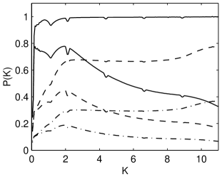
Figure 1: GW polarization degree ${\mathcal{P}}(K,t_{\rm{fi}})$, Eq. (3), as a function of scaled wave number $K=k/k_{S}$ relative to the large-scale wave number $k_{S}$ on which energy is pumped into the turbulence. This is evaluated at time $t_{\rm{fi}}$, after the turbulence has switched off, and remains unchanged to the present epoch. It has been computed for a damping wave number $k_{D}=10k_{S}$. Three pairs of curves are shown. Solid lines correspond to the amplitude ratio $A_{0}/S_{0}=1$ (maximally helical turbulence helicity2 ), dashed lines to $A_{0}/S_{0}=0.5$, and dot-dashed lines are for $A_{0}/S_{0}=0.2$. The upper line in each pair corresponds to HT turbulence with $n_{S}=n_{H}=-13/3$ MC96 ; DG01 and the lower line to HK turbulence with $n_{S}=-11/3$ and $n_{H}=-14/3$ L . Even for helical turbulence with $A_{0}/S_{0}\leq 0.5$, for large wave numbers $k\sim k_{D}$, $n_{S}=n_{H}=-13/3$ is unlikely so the large $K$ part of the lower dashed and dot-dashed HT curves are unrealistic. The large $k\sim k_{D}$ decay of the HK curves is a consequence of vanishing helicity transfer at large $k$ k73 .

Figure 1 and other numerical results show that for maximal helicity turbulence (when $A_{0}=S_{0}$) with equal spectral indices $n_{H}=n_{S}<-3$, the polarization degree ${\mathcal{P}}(k)\simeq 1$ (upper solid line). For weaker helical turbulence (when $A_{0}<S_{0}$) with $n_{H}\simeq n_{S}<-3$, ${\mathcal{P}(k)}\rightarrow CA_{0}/S_{0}$, where $1<C(n_{S},n_{H})<2$ is a numerical factor that depends on the spectral indices. For HT turbulence with $n_{S}=n_{H}=-13/3$, $C\approx 1.50$, while for Iroshnikov-Kraichnan MHD turbulence ($n_{S}=n_{H}=-7/2$), $C\approx 1.39$. Excluding the edges of the inertial range $k_{S}<k<k_{D}$, an analysis of Eqs. (10) and (11) shows that the main contribution to the integrals come from areas with $p_{1}\sim k_{S},~{}p_{2}\sim k$ and $p_{1}\sim k,~{}p_{2}\sim k_{S}$. In this case (for arbitrary spectral indices $n_{S}$, $n_{H}<-3$) $H(k),~{}{\mathcal{H}(k)}\propto k^{n_{S}-3}k_{S}^{n_{S}+3}$, so this approximate analysis indicates that ${\mathcal{P}(k)}$ is not very sensitive to $k$.

In position space, we find

$$\langle|h^{\pm}({\mathbf{x}},t_{\rm{fi}})|^{2}\rangle\simeq-\frac{9\alpha\tau S_{0}^{2}k_{S}^{n_{S}+3}}{64\pi^{4}(n_{S}+3)}\int_{k_{S}}^{k_{D}}dk(1\pm{\mathcal{P}}(k))k^{n_{S}-1}.$$ (12)

GW amplitudes are conventionally expressed as $\langle h^{ij}({\mathbf{x}},t_{\rm{fi}})h^{ij}({\mathbf{x}},t_{\rm{fi}})\rangle=2\int_{0}^{\infty}d{\rm{ln}}f[|h^{+}(f)|^{2}+|h^{-}(f)|^{2}],$ see Eq. (11) of Ref. m00 , where the frequency $f$ of a GW generated by an eddy of length $L$ is $f=\tau_{L}^{-1}$ where $\tau_{L}$ is the eddy turnover time kos ; kmk02 ; dolgov . This is inversely proportional to the cosmological scale factor, so the frequency ${\bar{f}}$ today and $f$ when the temperature was $T_{\rm{in}}=100~{}T_{100}$ GeV are related by ${\bar{f}}=1.65\times 10^{-5}T_{100}g_{100}^{1/6}f/H_{\rm{in}}$ Hz m00 , where $g_{\rm{in}}=100g_{100}$ is the number of relativistic degrees of freedom at $t_{\rm{in}}$. Since we truncate turbulence power for $L>L_{S}$, the GW spectrum is non-zero only for ${\bar{f}}>{\bar{f}}_{S}$, where

$${\bar{f}}_{S} = 1.9\times 10^{-6}\sqrt{\frac{n_{S}+5}{|n_{S}+3|}}\left(\frac{{\bar{\varepsilon}}}{\nu}\right)^{{1}/{2}}\left(\frac{L_{D}}{L_{S}}\right)^{(n_{S}+5)/{2}}$$ (13)

$$\times T_{100}~{}g_{100}^{{1}/{6}}~{}H_{\rm{in}}^{-1}~{}{\mbox{Hz}}$$

is the frequency now that corresponds to the stirring length $L_{S}$. Here we use the fact that for locally isotropic turbulence the energy dissipation rate ${\bar{\varepsilon}}=2\nu\int_{k_{S}}^{k_{D}}dk~{}k^{4}P_{S}(k)/\pi^{2}$ (where $\nu$ is the plasma viscosity, p. 483 of Ref. my75 ), is equal to the source power input, i.e., ${\bar{\varepsilon}}=3\kappa\rho_{\rm{vac}}/(4\rho\tau)$ and $\kappa$ is the phase transition efficiency. For HK turbulence with $n_{S}=-11/3$, Eq. (13) is Eq. (53) of Ref. kmk02 .

Using Eqs. (12) and (13), and neglecting the weak $k$-dependence of the GW polarization degree ${\mathcal{P}}$, we find that $h^{\pm}({\bar{f}})\propto{\bar{f}}^{-11/4}$ for the HK case kmk02 ; dolgov , while for HT turbulence $h^{\pm}({\bar{f}})\propto{\bar{f}}^{-13/2}$. We expect such a steeper dependence on frequency for helicity induced GWs, since the helicity transfer rate is more important on larger scales k73 . In both cases the amplitude of the GW spectrum peaks at the stirring frequency ${\bar{f}}_{S}$.

We close with a brief examination of the prospect of detecting such circularly polarized GWs. The GW energy density parameter for frequency ${\bar{f}}$, $\Omega_{\rm{GW}}({\bar{f}})$ is given by (see Eq. (7) of Ref  m00 ) $\Omega_{\rm{GW}}({\bar{f}})h^{2}=5.9\times 10^{35}(|h^{+}({\bar{f}})|^{2}+|h^{-}({\bar{f}})|^{2})({\bar{f}}/\mbox{Hz})^{2}$, where $h$ is the Hubble constant in units of $100$ km sec^-1 Mpc^-1. In our case,

$$\Omega_{\rm{GW}}({\bar{f}})h^{2}\simeq 1.05\times 10^{-11}~{}g_{100}^{-{1}/{3}}\left(\frac{L_{S}^{2}}{\tau H_{\rm{in}}^{-1}}\cdot\frac{n_{S}+5}{|n_{S}+3|}\right)^{2}$$

$$\times\left(\frac{L_{D}}{L_{S}}\right)^{3(n_{S}+5)}\left(\frac{3\kappa\rho_{\rm{vac}}L_{S}}{4\nu\rho}\right)^{3}\left(\frac{\bar{f}}{\bar{f}_{S}}\right)^{2(2n_{S}+5)/(n_{S}+5)}\!\!\!\!\!\!\!\!\!\!\!\!\!\!\!\!\!\!\!\!\!\!\!\!\!\!\!\!\!\!\!\!\!\!\!.$$ (14)

The stirring frequency ${\bar{f}}_{S}$ and the GW spectrum are very sensitive to phase transition properties. If the phase transition is strongly first order, for the HK case ${\bar{f}}_{S}\simeq 5\times 10^{-3}$Hz near the Laser Interferometer Space Antenna (LISA) frequency range, but the amplitude $\Omega_{\rm{GW}}({\bar{f}})h^{2}\simeq 10^{-11}$ kmk02 ; dolgov is below LISA sensitivity on this frequency nic ; tasi . An additional limit of detectability is imposed by the dominating stochastic GWs signal from white dwarf binaries white-dwarf . Thus it is unlikely that the GWs discussed here will be detected by currently planed GW detectors, but future detector configurations GWdetection may well be able to.

References

• (1) A. Buonanno, in Particle Physics And Cosmology: The Quest For Physics Beyond The Standard Model(s), eds. H. E. Haber and E. Nelson, (World Scientific, Singapore, 2004), p. 855.
• (2) A. Starobinsky, JETP Lett. 30, 682 (1979), Sov. Astron. Lett. 9, 302 (1983); V. Rubakov, M. Sazhin, and A. Veryaskin, Phys. Lett. B 115, 189 (1982); B. Ratra, Phys. Rev. D 45, 1913 (1992); M. Giovannini, Phys. Rev. D 60, 123511 (1999).
• (3) M. Kamionkowski, A. Kosowsky, and M. S. Turner, Phys. Rev. D 49, 2837 (1994); R. Apreda, et al., Class. Quant. Grav. 18, L155 (2001).
• (4) D. Deriagin, D. Grigor’ev, V. Rubakov, and M. Sazhin, Mon. Not. R. Astron. Soc. 229, 357 (1987); M. Giovannini, Phys.  Rev.  D.  61, 063004 (2000),  A. Lewis, Phys.  Rev.  D. 70, 043011 (2004).
• (5) A. Kosowsky, A. Mack, and T. Kahniashvili, Phys. Rev. D 66, 024030 (2002).
• (6) A. D.  Dolgov, D. Grasso, and A. Nicolis, Phys. Rev. D 66, 103505 (2002).
• (7) A. Nicolis, Class.  Quantum  Grav. 21, L27 (2004).
• (8) J. M. Cornwall, Phys.  Rev.  D 56, 6146 (1997);  T. Vachaspati, Phys.  Rev.  Lett. 87, 251302 (2001);  A. Brandenburg, Astrophys. J. 550, 824, (2001).
• (9) R. Banerjee and K. Jedamzik, Phys. Rev. D 70, 123003 (2004);  M. Christensson, M. Hindmarsh, and A. Brandenburg, Astron. Nachr. 326, 393 (2005).
• (10) T. Kahniashvili and B. Ratra, Phys. Rev. D 71, 103006 (2005).
• (11) C. Caprini, R. Durrer, and T. Kahniashvili, Phys. Rev. D 69, 063006 (2004).
• (12) D. H. Lyth, C. Quimbay, and Y.  Rodriguez, JHEP, 03, 016 (2005).
• (13) C. Misner, K. S. Thorne, and J. A. Wheeler, Gravitation (W. H. Freeman, San Francisco, 1973), Sec. VIII.
• (14) S. Kobayashi and P. Mészáros, Astrophys. J. Lett. 585, L89 (2003).
• (15) L. Pogosian, T. Vachaspati, and S. Winitzki, Phys.  Rev.  D 65, 083502 (2002).
• (16) M. Lesieur, Turbulence in Fluids (Kluwer Academic, Dordrecht, 1997).
• (17) J. O. Hinze, Turbulence (McGraw Hill, New York, 1975).
• (18) R. H. Kraichnan, J. Fluid Mech., 59, 745 (1973).
• (19) S. S. Moiseev and O. G. Chkhetiani, JETP 83, 192 (1996)].
• (20) V. Borue and S. A. Orszag, Phys. Rev. E 55, 7005 (1997).
• (21) P. D. Ditlevsen and P. Giuliani, Phys. Rev. E 63, 036304 (2001).
• (22) A. S. Monin and A. M. Yaglom, Statistical Fluid Mechanics: Mechanics of Turbulence, Vol. 2 (MIT Press, Cambridge, MA, 1975).
• (23) M. Maggiore,  Phys.  Rept. 331, 283 (2000).
• (24) A. Farmer and S. Phinney, Mon. Not. R. Astron. Soc. 346, 1197 (2003).
• (25) C. Ungarelli and A. Vecchio, Phys. Rev. D 63, 064030 (2001); C. J. Hogan and P. L. Bender, Phys. Rev. D 64, 062002 (2001); N. Seto and A. Cooray, Phys. Rev. D 70, 123005 (2004).