Deep ACS Imaging of the Halo of NGC 5128: Reaching the Horizontal Branch

Abstract

Using the HST Wide Field Camera (WFC) of the Advanced Camera for Surveys (ACS), we have obtained deep $(V,I)$ photometry of an outer-halo field in NGC 5128, to a limiting magnitude of $I\simeq 29$. Our photometry directly reveals the core helium-burning stellar population (the “red clump” or horizontal branch) in a giant E/S0 galaxy for the first time.

The color-magnitude diagram displays a very wide red giant branch (RGB), an asymptotic giant branch (AGB) bump, and the red clump; no noticeable population of blue HB stars is present, confirming previous suggestions that old, very metal-poor population is not ubiquitous in the halo of this galaxy. From the upper RGB we derive the metallicity distribution, which we find to be very broad and moderately metal-rich, with average $\mathrm{[M/H]}=-0.64$ and dispersion $0.49$ dex. The MDF is virtually identical to that found in other halo fields observed previously with the HST, but with an enhanced metal-rich population which was partially missed in the previous surveys due to $V$-band incompleteness for these very red stars. Combining the metallicity sensitive colors of the RGB stars with the metallicity and age sensitive features of the AGB bump and the red clump, we infer the average age of the halo stars to be $\sim 8^{+3}_{-3.5}$ Gy.

As part of our study, we present an empirical calibration of the ACS $F606W$ and $F814W$ filters to the standard $V$ and $I$ bands, achieved with ground-based observations of the same field made from the EMMI camera of the New Technology Telescope of the ESO La Silla Observatory.

1 Introduction

A significant fraction of all the stars in the Universe reside within giant elliptical galaxies, yet the formation epochs of these large systems are still a matter of debate. The three main elliptical galaxy formation processes are generally considered to be: (i) in situ conversion of protogalactic gas through multiple starbursts (e.g. Partridge & Peebles, 1967; Tinsley, 1972; Larson, 1974; Harris et al., 1995), (ii) later mergers of pre-existing disk galaxies (e.g. Toomre, 1977; Ashman & Zepf, 1992; Kauffmann et al., 1993; Cole et al., 2000), and (iii) ongoing accretion of small satellites (e.g. Coté et al., 1998). The three models predict different mean ages; they also predict different metallicities and metallicity gradients for the stars that build these galaxies, as well as different distributions and characteristics of the (multiple) globular cluster populations.

Elliptical galaxy formation studies are generally based on observations of high-redshift populations, or deductions of mean ages and metallicities of nearby systems from measurements of their integrated spectral indices (e.g. Trager et al., 2000; Kuntschner et al., 2002; Dressler et al., 2004). In recent years the availability of high-multiplex instruments at large aperture telescopes makes the study of globular clusters and planetary nebulae in these galaxies a promising new tool (e.g. Walsh et al., 1999; Romanowsky et al., 2003; Puzia et al., 2004; Peng et al., 2004a, b). At the same time, it has now become possible to study the resolved stellar populations in elliptical galaxies directly – an important complementary approach to the study of the high-redshift Universe, and integrated stellar and globular cluster light.

But even with the best available imaging tools (HST, VLT, Gemini), resolving the old halo stars is possible for only the nearest E/S0 galaxies. Pioneering work of this type was done notably for the halos of large E/S0 systems including NGC 5128 (Soria et al., 1996), Maffei 1 (Davidge & van den Bergh, 2001), NGC 3379 (Gregg et al., 2004), NGC 3115, NGC 5102, and NGC 404 (Schulte-Ladbeck et al., 2003). Hence, these few objects provide the irreplaceable chance for calibrating all the techniques that involve integrated spectral indices and population synthesis. Moreover they provide the only way to measure the properties of stellar populations in the outer halo, while the integrated light measurements refer to the central areas.

At a distance of 3.8 Mpc NGC 5128 (commonly referred to as Centaurus A) is by far the nearest easily observable E/S0 galaxy (Harris et al., 1999; Rejkuba, 2004), and is thus a uniquely valuable testing ground for stellar population and galaxy formation models. Its halo light was first resolved in stars by Soria et al. (1996) using the HST/WFPC2 camera. Further, deeper WFPC2 photometry, reaching 2.5 magnitudes down the red giant branch (RGB), was carried out by Harris et al. (1999) and Harris & Harris (2000, 2002) in the optical $V$ and $I$ bands, and by Marleau et al. (2000) with the near-infrared NICMOS camera in $J$ and $H$. Using ground-based data, Rejkuba et al. (2001, 2003) presented deep color-magnitude diagrams (CMDs) in $V$, $J$, $H$, and $K_{s}$ with FORS1 and ISAAC at the VLT.

All these earlier studies indicated that the halo of this giant E/S0 galaxy is dominated by the presence of normal RGB stars, demonstrating that the halo stars are at least a few Gy old. The same RGB photometry provides the means to construct the metallicity distribution function (MDF) of its halo stars. However, relatively little is yet known about the age distribution function (ADF) of its halo stars. There is ongoing star formation in the north-eastern halo fields along the galaxy’s major axis (Graham, 1998; Mould et al., 2000; Fassett & Graham, 2000; Rejkuba et al., 2001; Graham & Fassett, 2002; Rejkuba et al., 2002), but simulations show that the star formation rate in this area has been lower than in the solar neighborhood and comparable to some Local Group dIrr galaxies, hence contributing relatively little to the stellar halo mass (Rejkuba et al., 2004). A suggestion that this galaxy had an appreciable intermediate-age component was raised in the early work of Soria et al. (1996) and Marleau et al. (2000), but was contested later with observations of different halo fields (Harris et al., 1999; Harris & Harris, 2000, 2002) which indicated no need for any significant contribution of intermediate-age or young components in the halo. However, the extended giant branch observed in the $V,K$ CMD (Rejkuba et al., 2001) and the presence of long-period variable AGB stars with periods in excess of 450-500 days (Rejkuba et al., 2003), seem to confirm that up to $\sim 10$% of the halo might consist of an intermediate-age population in the range $\sim 3-7$ Gy. Additional lines of evidence for an intermediate-age component come from recent photometry and spectroscopy of the NGC 5128 globular cluster system (Peng et al., 2004b; Yi et al., 2004).

The Advanced Camera for Surveys (ACS; Ford et al., 1998) installed on HST during the servicing mission 3B in March 2002 has made it possible to investigate stellar populations to both significantly deeper limits and higher resolution. With ACS, it is now possible in NGC 5128 to reach the red clump and the horizontal branch (the old core-helium-burning stars) and the asymptotic giant branch (AGB) bump directly. Since these features are sensitive to both metallicity and age, we can examine quantitatively and directly the ADF of the halo stars in a giant E/S0 galaxy for the first time. In this paper we present a very deep color-magnitude diagram (CMD) of a remote halo field in NGC 5128, showing the AGB bump, red clump and the horizontal branch in NGC 5128. Simple comparisons of the observed and simulated luminosity functions are used to obtain an average age for the halo stars. In a following paper we plan to present a more thorough simulation of the CMD and derive from it a star formation history (SFH).

Throughout the paper we use an intrinsic distance modulus for NGC 5128 of $(m-M)_{0}=27.92$ (Rejkuba, 2004) and a reddening of $E(B-V)=0.11$ (Burstein & Heiles, 1982; Schlegel et al., 1998).

2 The Data

2.1 HST Observations and Photometry

For the deep HST ACS observations of the NGC 5128 halo we chose a field centered at $\alpha_{\mathrm{J2000}}=13^{\mathrm{h}}25^{\mathrm{h}}15\fs 1,\delta_{\mathrm{J2000}}=-43^{\circ}34\arcmin 30\arcsec$, a projected distance of some $33\farcm 3$ to the south of the galaxy center. This location corresponds to a linear projected distance of 38 kpc. The choice of such a remote halo location was driven by the requirements to have low surface brightness, i.e. low enough stellar density to permit high precision photometry, unaffected by crowding, but still give a high enough number of stars to make up a large statistical sample. We also avoided, as much as possible, the obvious bright foreground stars which would saturate in long exposures. This latter criterion proved to be an issue with the combination of the low galactic latitude of NGC 5128 and the high sensitivity of the new camera. Additionally the target field was chosen to avoid any peculiarities of this galaxy, like jet induced star forming regions (Mould et al., 2000; Rejkuba et al., 2002), shells (Malin et al., 1983), and dust lanes (Stickel et al., 2004).

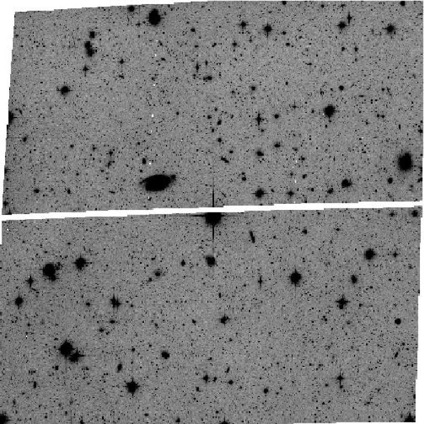
Figure 1: Combined image consisting of 12 V and 12 I full-orbit exposures. The total exposure time is more than 19 h. The faintest stars in this image have $V\sim 30$ and $I\sim 29$ mag.

The ACS observations were taken in Cycle 11 between 2002 July 5 and 9 within GO program 9373. They consist of 12 full orbit exposures in F606W (broad $V$), divided among 4 visits, and 12 full orbit F814W ($I$) exposures, also divided among 4 visits. The first exposure in each visit was 2520 sec, while all the others were 2600 sec long. Hence the total exposure times amount to $4\times 2520+8\times 2600$ sec, or 8.58 h for each filter. The individual exposures were not dithered, but the pointing differences between the different visits resulted in shifts between images of up to 4 pix, which, combined with 12 exposures per filter, enabled us to remove the cosmic rays and hot pixels efficiently by registering and combining the individual frames. The very deep median combined image made from all the exposures is shown in Fig. 1.

The data were processed with the on-the-fly CALACS pipeline which included dark and bias subtraction, flatfielding and geometric distortion correction, but no cosmic ray rejection. We used the pipeline reduced “drz” images for photometry with the following steps. First, we multiplied each image by the corresponding exposure time. Then we ran standard PSF photometry with the DAOPHOT suite of codes (Stetson, 1987, 1994). The PSF for each individual exposure was determined with the spatially variable option and $65-90$ non-saturated, relatively isolated stars that did not suffer from many cosmic ray hits. The PSFs from the 12 $F606W$ and 12 $F814W$ images were then combined into a single PSF per filter using the MULTIPSF program. The FIND+PHOT+ALLSTAR programs were followed by DAOMATCH and DAOMASTER in order to determine accurate geometric transformations between the images, and then all the images (both in F606W and F814W filters) were combined together with MONTAGE2. Using the resulting deep, cleaned image (Fig. 1) we constructed an initial photometry list of 70586 candidate stars, which was then used as a coordinate input for ALLFRAME. The resulting photometry for 65000 stars in both images was used to determine new, improved geometric transformations between images, with the requirement to detect the same star on all the images and adopting stringent photometric quality ($\sigma<0.05$). All of the 24 frames were then combined again and we made two runs of FIND+PHOT+ALLSTAR to define a final input list of 93812 stars for ALLFRAME. The increase in the number of detected stars on the combined image is due to much improved transformations which were based on more than 60000 stars compared to the few hundred that could be detected on individual images in the first run of ALLSTAR.

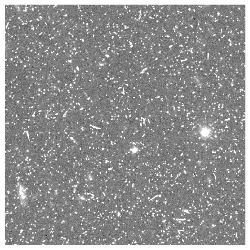
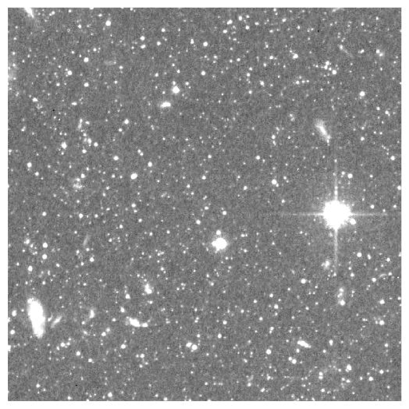
Figure 2: Left panel: a $45^{\prime\prime}\times 43^{\prime\prime}$ portion of one F606W image. Most of the sources visible are cosmic rays. Right panel: The same part of the observed field as on the left is show this time as a combined image consisting of all 12 F606W and 12 F814W exposures. The total exposure time is more than 19 h. A large number of background galaxies is visible. They are rejected from our final photometry catalogue by very stringent photometric selection criteria.

It should be noted that the long individual exposure times meant that all the images were affected by a very large number of cosmic rays. An example of a small portion of one $F606W$ exposure is shown in the left panel of Fig. 2. The final combined image of the same $45^{\prime\prime}\times 43^{\prime\prime}$ field is in the right panel. The cosmic rays were not removed prior to ALLFRAME PSF photometry. The stars were detected on the basis of their matched coordinates. The final photometry catalogue contains 93306 F814W and 93067 F606W sources detected on at least 6 frames of each filter. The requirement to detect a star in at least 6 frames effectively rejects all the cosmic rays located near or on images of real stars in the field. The mean magnitude and the associated error were calculated for all the stars for each filter and then the two lists were matched with the requirement that the star is detected in both filters.

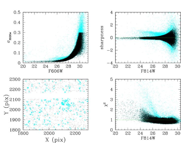
Figure 3: Photometry selection criteria based on photometric error, sharpness and $\chi^{2}$ parameters from DAOPHOT programs are plotted as function of F606W and F814W magnitudes and positions on the chip. Only sources lying within two hyperbolic envelopes around the sharpness value of zero (upper right panel) and to the right of the maximum allowed $\sigma$ at a given magnitude (upper left panel), as well as having $\sigma<0.3$ and $\chi^{2}<3$ and $-2<sharpness<2$ are considered “good” stars. They are plotted with black dots in all the panels. The sources that did not satisfy the above criteria are plotted with light gray dots (cyan color in electronic edition) and were rejected from the final photometric catalogue. In the lower left panel we show that these selection criteria effectively reject all the noise spike detections around a saturated star: a large number of gray (cyan) crosses around (x, y)=(2100, 2080) corresponds to a very saturated foreground star.

Additional selection criteria were applied, as illustrated in Fig. 3, on DAOPHOT parameter sharpness and on $\sigma$ (photometric error). The sharpness parameter estimates the intrinsic angular size of the measured objects. It is roughly defined as the difference between the square of the width of the object and the square of the width of PSF and has values close to zero for single stars, large positive values for blended doubles and partially resolved galaxies, and large negative values for cosmic rays and blemishes. We chose as “good” stars those sources lying within two hyperbolic envelopes around the sharpness value of zero (upper right panel of Fig. 3) and to the right of the maximum allowed $\sigma$ at a given magnitude (upper left panel). The remaining cosmic ray blemishes and resolved background galaxies were then rejected. Additionally we restricted the maximum allowed absolute value of the sharpness parameter to 2 (upper right panel), of $\sigma$ to 0.3 (upper left panel) and of $\chi^{2}$ to 3 (lower right panel). In the lower left panel of Fig. 3 we show that these selection criteria effectively reject all the noise spike detections around a saturated star (a large number of gray crosses around (x, y)=(2100, 2080) corresponds to a severely saturated foreground star). Also, it can be seen that the crowding is not excessive, hence allowing good sky subtraction and reliable photometry. These final selections resulted in a total of 77810 objects detected and measured in the entire field.

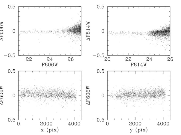
Figure 4: Comparison between our final photometric catalogue and the photometry done on a subset of flatfielded, but not drizzled images.

As suggested by the referee, we have checked our photometry against a reduction based on a subset of flatfielded, but not drizzled images. The reduction of “flt” images was done as described in Bedin et al. (2005), and the comparison is shown in Fig. 4. The small offset between the measurement done on “flt” and “drz” images may come from the difference in the aperture correction. Any systematic effects are smaller than 0.01 mag. The larger scatter for fainter magnitudes is due to smaller number of “flt” images. This comparison shows that the process of drizzling, which results in adjacent pixels being correlated, has not affected the precision of our photometry.

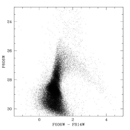
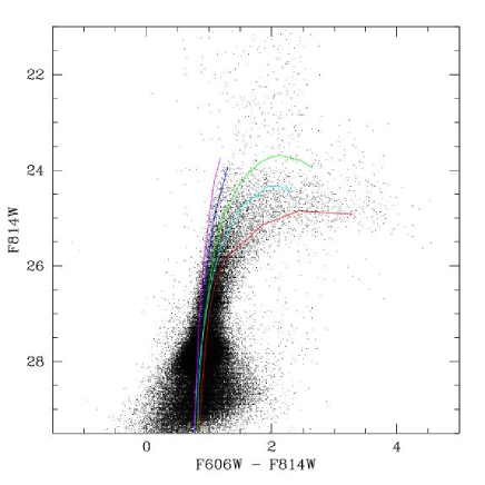
Figure 5: Left panel: F606W-F814W vs. F606W CMD calibrated to VEGAmag HST system. Right panel: F606W-F814W vs. F814W CMD calibrated to VEGAmag HST system. Overplotted are RGB fiducials derived from the ACS observations with the same filters by (Bedin et al., 2005).

To calibrate the photometry to the VEGAmag HST photometric system we adopted the zeropoints from the ACS web page (December 2003), namely 26.385 mag for F606W and 25.487 mag for F814W. An aperture correction of -0.09 mag in both filters was adopted to scale magnitudes from $0\farcs 5$ to an infinite radius (M. Sirianni, private communication). The CMDs calibrated to the VEGAmag system are presented in Fig. 5. Overplotted on the $F814W~{}vs.~{}(F606W-F814W)$ CMD are RGB fiducials from Bedin et al. (2005) derived from fits to the Galactic globular clusters NGC 6341, NGC 6752, NGC 104 (47 Tuc), NGC 5927, and NGC 6528 observed with ACS in the same photometric bands (Brown et al., 2003). These clusters span a range of metal abundances from $-2.2$ dex up to Solar metallicity. Already in this figure the large range of metal-abundances among the halo stars in NGC 5128 can be appreciated. We note that the RGB ridge line for NGC 104, which has intermediate metallicity between metal-poor (NGC 6341 and NGC 6752) and metal-rich clusters (NGC 5927 and NGC 6528) appears to extend to much brighter magnitudes than other clusters. This is not the case when the comparison is made in $V$ and $I$ bands and deserves clarification, which is beyond the scope of the present paper. The calibration of the photometry to the standard ground based $V$ and $I$-bands is described below.

2.2 Ground Based Observations and Photometry

For the purposes of obtaining an empirical calibration of the ACS photometry to the ground based system, on Aug. 1 2003, we obtained $5\times 330$ sec $V-$band exposures and $4\times 320$ sec $I-$band exposures in our ACS target field using the EMMI optical imager at the New Technology Telescope (NTT) at the ESO La Silla Observatory (Dekker et al., 1986). We used the red arm of EMMI (RILD), which has a $9.0^{\prime}\times 9.9^{\prime}$ field of view; we also used $2\times 2$ binning giving an image scale $0\farcs 33/\mathrm{pix}$. The weather was photometric and seeing was 1.2 arcsec.

The reduction procedure for the EMMI data involved bias subtraction and division by normalized twilight flat field images. Individual dithered exposures taken with the same filter were then shifted and combined into a single deep image in each filter on which photometry was performed with DAOPHOT (Stetson, 1987). A spatially variable PSF was constructed for both images using more than 60 stars. Only one cycle of FIND+PHOT+ALLSTAR was run as the fainter stars did not have sufficient photometric accuracy for calibration.

The calibration of the EMMI photometry was established from 57 stars in 3 Landolt fields (Landolt, 1992; Stetson, 2000) PG1525, PG2331, and SA 111, all observed on the same night. The following photometric solution was derived:

$$v = V-26.002(\pm 0.043)+0.125(\pm 0.036)*Airmass$$ (1)

$$i = I-25.614(\pm 0.046)+0.054(\pm 0.035)*Airmass$$ (3)

$$+0.040(\pm 0.011)*(V-I)$$

where $v$ and $i$ are instrumental magnitudes and $V$ and $I$ are magnitudes from the Stetson (2000) catalogue. The $1\sigma$ scatter around the mean is 0.034 mag for both filters. Including the color term in the $V$-band equation does not reduce the scatter, and the error in the color term is larger than its value, hence we prefer not to include it.

3 Calibration of the ACS $F606W$ and $F814W$ photometry

Most of the stars observed with EMMI belong to the foreground Galactic population. Given the exposure times, these stars are quite bright and some are saturated on the ACS images. The match between the ACS and EMMI catalogs was obtained with the IRAF task GEOMAP and was further refined with DAOMASTER (Stetson, 1987). The matched sources in both images number just 119 and each one of them was visually inspected. This resulted in rejection of 52 matched sources, either because they were extended or double on the ACS and single on EMMI images, or because they were saturated in the ACS image.

Finally, using 67 best matches between the EMMI and ACS frames we derive the following transformation equations using least-squares fitting with an iterative $3\sigma$ rejection algorithm:

$$(V-F606W) = 0.222(\pm 0.010)\times(V-I)$$ (5)

$$+0.072(\pm 0.016)~{}\quad\quad rms=0.046$$

$$(I-F814W) = -0.042(\pm 0.010)\times(V-I)$$ (7)

$$+0.130(\pm 0.016)~{}\quad\quad rms=0.050$$

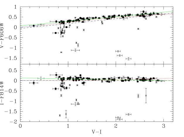
Figure 6: Empirical calibration of the ACS photometric system (F606W and F814W) into the $V$ and $I$ bands. All the 119 matching sources between the ACS and EMMI images are plotted with error-bars, and 67 stars used to derive the calibration are plotted with filled symbols. Solid lines (green color in electronic edition) are our linear fits used to derive the transformations in Eq. 7. Overplotted for comparison are also transformations from Sirianni et al. (PASP, submitted) derived from synthetic photometry (dotted blue and red lines) and observations (dashed black lines).

The $1\sigma$ scatter around the fit (not including points rejected from the fit) is shown on the right side of each equation. We show these fits in Fig. 6 with solid lines, where we plot all the matched sources between ACS and EMMI images with error-bars; those that passed the visual inspection (67 stars), and were thus used in fitting are plotted with filled dots. The (x, y) positions from the $F814W$ ACS image, $F606W$ and $F814W$ magnitudes in the VEGAmag system, as well as $VI$ magnitudes from EMMI and positions for all these 67 stars are listed in Tab. 1.

For comparison in Fig. 6 overplotted are also the transformations between the ACS WFC bands and ground based VI photometry derived by Sirianni et al. (submitted). Dotted lines (blue and red respectively) are used for transformations derived from synthetic photometry for blue and red stars, while the dashed lines show the transformations of derived from the observations (see Sirianni et al. for details).

3.1 Completeness and Error Analysis

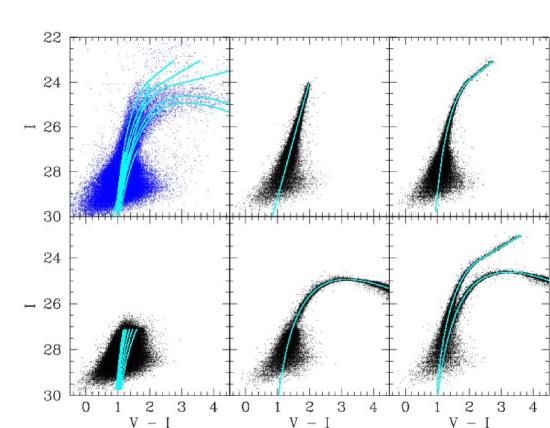
Figure 7: Upper left panel: observed color-magnitude diagram with simulated RGB sequences overplotted in light gray (cyan color in electronic edition). In the other panels some of the simulated color-magnitude diagrams are shown, indicating the scatter due to photometric errors and incompleteness as a function of magnitude and color. In order to reproduce the full width of the lower RGB it was necessary to simulate RGB sequences with a wide range of colors corresponding to $-2<[Fe/H]<0.0$ as shown in the lower left panel.

The measured CMD distribution in principle suffers from both incompleteness at the faint end due to loss of faint stars and an excess at the bright end due to blends of two or more bright stars. Completeness of our ACS photometry has been evaluated from normal artificial star techniques. Many test runs were made, in each one of which we added more than 22000 stars to all the images distributed evenly on a grid with minimum separation of 2.1 effective PSF radii between the added stars in order not to increase the crowding. The starting pixel of the grid was varied randomly in each run. In total, 341400 simulated stars were added in 15 experiments. Figures 7 to 10 illustrate the results of the completeness and error analysis.

The input magnitudes and colors of the artificial stars were chosen along sequences which correspond to the red giant stars in Galactic globular clusters spanning a range of metallicities $-2<\mathrm{[M/H]}<0.0$ dex, computed using the analytical expressions from Saviane et al. (2000). In some cases these analytic RGB sequences were extrapolated to magnitudes brighter than the RGB tip magnitude in order to probe the completeness and photometric error of the upper part of the CMD where AGB stars may be expected. The input sequences are shown in light gray in the upper left panel of Fig. 7 superimposed to the CMD of our ACS field (black dots). The other panels of Fig. 7 illustrate the effect of the photometric errors and incompleteness on the CMD by showing both the input sequences (in light gray) and the output magnitudes and colors (in black). Several completeness experiments were made using only faint part of RGB loci as input magnitudes and colors to gain larger statistics in the part of the CMD where the errors and completeness vary most. Clearly the wide color range of the stars in our field requires a wide range in metallicity. This is evident both in the upper part of the RGB, and at the fainter magnitudes, as shown in the lower left panel.

The photometric completeness is defined here as the fraction of recovered objects at a given magnitude $f=N_{measured}/N_{simulated}$. We specify that the simulated star is considered to be recovered if its position is measured within 1 pixel of the input position and its magnitude within 0.75 mag of the input magnitude (corresponding to blending of up to 2 stars with the same magnitude). Fleming et al. (1995) show that the completeness function can be well fitted with the following analytical function:

$$f=\frac{1}{2}\left[1-\frac{\alpha(m-m_{0})}{\sqrt{1+\alpha^{2}(m-m_{0})^{2}}}\right]$$ (8)

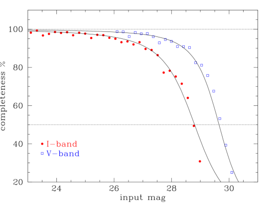
Figure 8: Completeness as a function of magnitude can be well fitted with the analytic function for simulated stars with $V-I$ colors bluer than $\sim 2.5$. This figure is a plot of completeness fraction as a function of magnitude for simulations with input colors bluer than $V-I=1.5$. The fit has the following parameters (see eq. 8): $\alpha(V)=1.1$, $m_{0}(V)=29.65$, $\alpha(I)=0.82$ and $m_{0}(I)=28.80$.

In our case, given the very wide range of colors at a given magnitude, the completeness at a given magnitude is also a strong function of color. Figure 8 shows the results of the completeness test limited to stars with input colors bluer than $V-I=1.5$, on which we superimpose the Fleming et al. relation with $\alpha\simeq 1.1$ for the $V$-band and 0.8 for the $I$-band. It can be seen that, for the blue stars, the analytic relations give a very good description of the data, and that the 50% completeness is reached at magnitude $m_{0}(V)=29.65$ and $m_{0}(I)=28.80$. Actually, these relations adequately describe the completeness for artificial stars with colors up to 2.5.

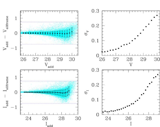
Figure 9: Mean error as a function of magnitude. On the left we plot difference between the measured and input magnitude as a function of input magnitude for all the stars from our completeness simulations with light gray (cyan in the electronic edition) dots, while the panels on the right show mean error as a function of magnitude as measured from these simulations. Only those simulated stars that were recovered within 1 pix of the input position and that had magnitudes within 0.75 of the input magnitude are considered to be recovered. There is no systematic shift of the mean magnitude difference and the typical $1\sigma$ errors at the 50% completeness magnitude limits are of the order of 0.3 mag.

The photometric errors, quantified as difference between the input and the output magnitude of the artificial stars, are shown in Figure 9. The mean magnitude difference $\Delta mag=mag_{simulated}-mag_{measured}$ is consistent with 0 for magnitudes brighter than a 70% incompleteness limit. The shift toward systematically brighter measured magnitudes, which signals the occurrence of blending of the stellar images is smaller than 0.09 mag at the magnitude bin corresponding to 50% incompleteness. The mean scatter, a measure of the photometric error, is smaller than 0.3 for all the magnitudes up to the 50% incompleteness level as shown also on the right panels of Figure 9.

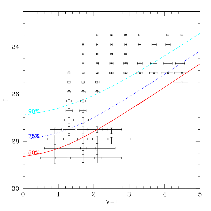
Figure 10: Mean error and completeness as a function of magnitude and color.

Finally, Fig. 10 summarizes the amplitude of the photometric errors and the completeness levels throughout the CMD of our field. It can be noticed that our data are fairly complete along the upper two magnitudes on the RGB over a very wide color range. At the level of the red clump (I=28, V-I=1) our data are still $\sim 70$% complete.

4 The Color-Magnitude Diagram

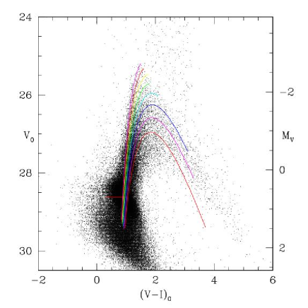
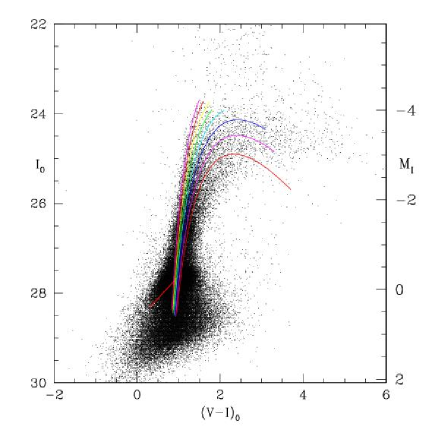
Figure 11: V vs. (V-I) and I vs. (V-I) CMDs calibrated to ground based system and de-reddened assuming $\mathrm{E}_{B-V}=0.11$. Overplotted are empirical fits to Galactic globular cluster RGBs ranging in metallicity from $-2\leq\mathrm{[Fe/H]}\leq-0.25$ in steps of 0.25 dex (Saviane et al., 2000). The short horizontal line indicates the position of the HB in 47 Tuc (Rosenberg et al., 2000). Foreground stars have colors $\mathrm{V}-\mathrm{I}\lesssim 3.5$ and are easily observed above the tip of the red giant branch stars in NGC 5128, which has magnitude $\mathrm{I}=24$. Stars brighter than the tip of the RGB and redder than $\mathrm{V}-\mathrm{I}\simeq 3.5$ are most probably metal-rich long period variable stars in NGC 5128 halo.

In Fig. 11 we plot the final CMD for our ACS field, calibrated to the ground-based $VI$ photometric system through the transformations above. In this figure as well as throughout the following discussion we have de-reddened the photometry assuming $E(B-V)=0.11$ (Schlegel et al., 1998) and the Cardelli et al. (1989) reddening law.

As expected from previous studies of the NGC 5128 halo (e.g. Harris et al., 1999; Harris & Harris, 2000, 2002), we find that the CMD is dominated by an old stellar population of RGB stars. At blue colors ($V-I\lesssim 2.5$) the RGB tip is well defined around $I\sim 24$, but at redder colors it bends over to fainter magnitudes up to $I\sim 25.2$ around $V-I=4.5$. According to our completeness simulations we do not expect to have missed many red objects. Inspection of our database shows that there is only one star-like object with $I<26$, and other two with $26<I<27$ that have not been detected on the $V$-band images.

Stars brighter than $I\sim 24$ mostly belong to the Galactic foreground population. It is easily seen that most of the Galactic stars have $0\lesssim(V-I)_{0}\lesssim 2.5$. The predicted number of foreground Galactic stars in the range of $I=22-24$ is $\sim 5$ arcmin^-2 (Bahcall & Soneira, 1981), yielding 57 stars in this magnitude interval in our 11.33 arcmin² ACS field. The Besançon group model of the Galaxy available through the Web (Robin et al., 1996) predicts 68 stars in this magnitude interval in our field and a total of 415 stars with magnitudes between $20<V<29$. This is negligible compared to the 77810 stars in our photometric catalogue, and even around magnitude bins where the red clump and AGB bump features are detected (see below) the Galactic contamination is of the order of 1% at most. Above the tip of the RGB, however, this contamination is significant. We observe 86 stellar sources between $22<I_{0}<24$ and $0\leq(V-I)_{0}\leq 2.5$. Most should be foreground Galactic stars, but a few could be long-period AGB variable stars. Finally, there are many stellar objects redder than $(V-I)>2.5$ and brighter than the tip of the RGB. These are most probably long period variable stars belonging to the metal-rich population, similar to those reported by Rejkuba et al. (2003) in other halo fields in NGC 5128.

At $I\sim 28$ the RGB becomes much wider and very much more heavily populated. We identify the excess of stars there as the red clump (RC): that is, core-helium burning stars, seen here for the first time in a giant E/S0 galaxy. In Fig. 11, the (red) short slanted line at $27<I<28$ and $V-I$ from 0.4 to 1.0 indicates the expected position of the horizontal-branch stars of 47 Tuc, the classic metal-rich Galactic globular cluster (Rosenberg et al., 2000), shifted to the distance modulus and reddening of NGC 5128. Notably, there is no trace of an extended blue horizontal branch, which would normally be found if an old metal-poor stellar population were present. However, we express a note of caution: the large incompleteness and photometric errors at these faint magnitudes may prevent a weak blue horizontal branch from being evident. At face value, the very low number of blue HB stars indicates either a relatively young mean age or a stellar population that has virtually no low-metallicity component. We argue for the latter conclusion in the discussion below.

In its general features, the CMD is strikingly similar to that of the lower-luminosity Local Group elliptical M32 (Grillmair et al., 1996). The luminosity functions for these two galaxies are compared in more detail below.

5 The Metallicity Distribution

Overplotted in Fig. 11 are empirical analytic fits to Galactic globular clusters RGBs with a wide range of metallicities from Saviane et al. (2000). Going from blue to red we plot the model RGBs from [M/H] = $-2$ to $-0.25$ dex in steps of $0.25$ dex. The lines trace rather well the metal-poor part of the RGB, but the two most metal-rich hyperbolas are obviously not adequate. It is evident that stars with almost-Solar metallicities are present even at this remote halo location (and it is worth emphasizing that the minimum true galactocentric distance of any stars in the target field is $r_{gc}=36$ kpc). Also, it should be noted that due to the very red colors of the most metal-rich giants, in order to sample the complete metallicity distribution, it is necessary to reach $V$-band magnitude limits of $\sim 29$. The ACS data achieve this much better than the earlier WFPC2 studies. We plot the distribution of V-I color along the RGB for magnitudes with completeness larger than 70% in Figure 12.

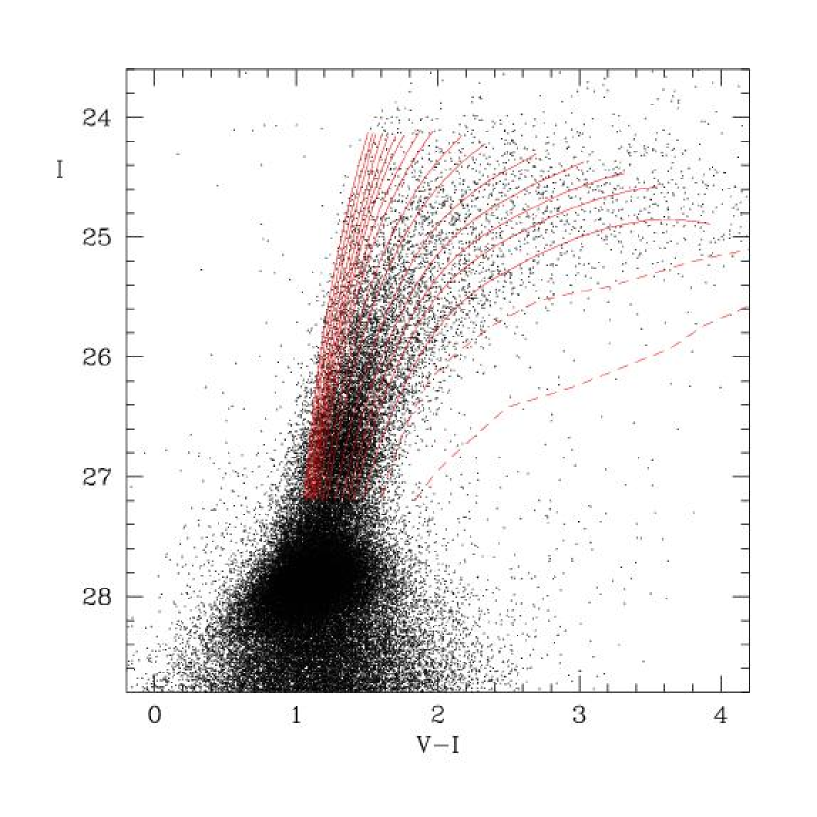
Figure 13: $VI$ CMD with overplotted theoretical models. The solid lines are 1 M_⊙ tracks from VandenBerg et al. (2000), empirically calibrated to match the RGB colors of Galactic globular clusters. The two dashed tracks are two metal-rich tracks defined as described by Harris & Harris (2002).

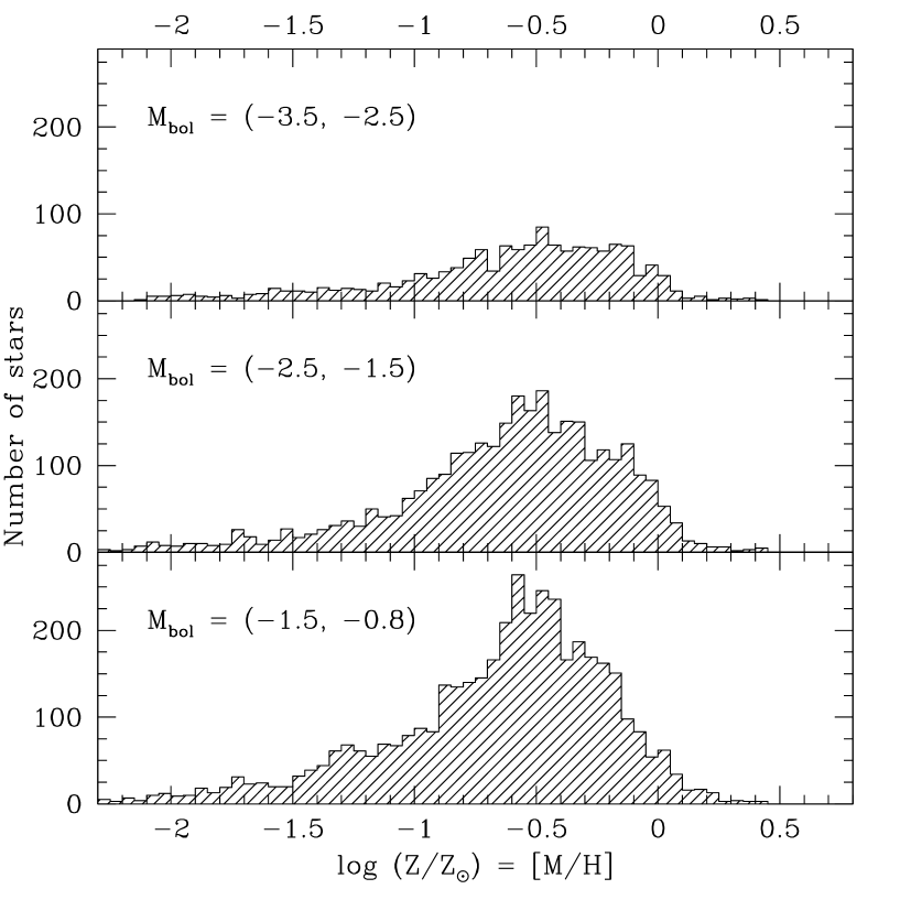
Figure 14: Metallicity distribution function for three different luminosity bins along the RGB are shown, from the top of the RGB down to more than 2.5 mag fainter. Very similar spread in the three magnitude bins shows that photometric errors are similar and that there is no significant incompleteness up to 2.5 mag fainter than the tip of the RGB.

In order to derive the MDF for this field we use the same procedure as for the other halo fields observed with WFPC2 (Harris & Harris, 2000, 2002). A finely spaced grid of red giant evolutionary tracks (VandenBerg et al., 2000), with colors calibrated using Galactic globular clusters, is overplotted on the CMD (Fig. 13). Interpolation within the grid is done in $[M_{bol},(V-I)_{0}]$ space (see Harris & Harris, 2002, for detailed method) to estimate the heavy-element abundance of each star on the upper part of the RGB. The resulting MDF, defined as number of stars per bin in log $(Z/Z_{\odot})$, is shown for three different magnitude bins covering the top part of the RGB where the photometric accuracy is highest (Fig. 14). Encouragingly, we see no trends in the MDF with magnitude, indicating that there are no luminosity-dependent effects in the interpolation.

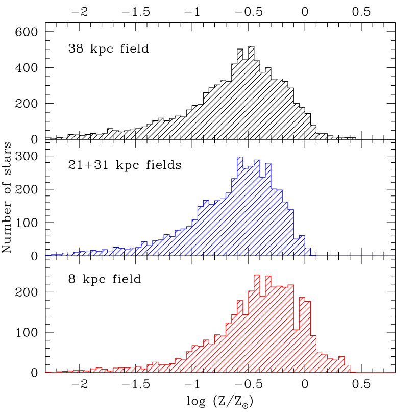
Figure 15: Comparison of MDF in the new ACS field (40 kpc), and in the previously observed inner halo fields: middle panel shows a combined MDF for 21 and 31 kpc fields (Harris & Harris, 2000) and the bottom panel is MDF for the inner (bulge) field at 8 kpc (Harris & Harris, 2002).

The combined MDF for all three bins is compared with those from the three other halo fields previously observed with WFPC2 (Harris et al., 1999; Harris & Harris, 2000, 2002), in Fig. 15. It is clear that our outermost ACS field has an MDF very similar to those of the mid-halo 21-kpc and 31-kpc WFPC2 fields. As noted in Harris & Harris (2002), the innermost 8-kpc field is significantly more metal-rich on average. On closer inspection, we see that the ACS field has a more well populated high-metallicity end than does the mid-halo MDF. We attribute this difference to the very large bolometric corrections for the reddest stars in our CMD, which make them extremely faint in $V$ and could have driven them below the (shallower) WFPC2 photometric limits (see Harris & Harris, 2002, for further discussion on this point, and attempts to derive a completeness-corrected MDF). A quantitative comparison between the mean metallicities in the three fields is presented in Table 2. Interestingly, Beasley et al. (2003) noted that their best hierarchical-merging formation model of a giant elliptical like NGC 5128 predicts a higher fraction of most metal-rich stars than were in the earlier CMDs, a conclusion acting in the same direction. These comparisons show the importance of getting very deep and accurate photometry to detect the most metal-rich part of the RGB.

Although the RGB color for “old” ($\sim$ 5 Gy or more) stellar populations is primarily sensitive to metallicity, some comments should be made about the potential effects of age differences within the sample (for a more detailed discussion see Salaris & Girardi, 2005). The grid of RGB tracks used to derive our MDF was normalized to the $(V-I)$ colors and luminosities of real globular clusters in the Milky Way (see Harris & Harris, 2000, 2002), and thus implicitly assumes a uniform age for the NGC 5128 halo population of about 12 Gy (that is, the same as the mean age for the classic Milky Way GCs). What if the population is significantly younger? To test the effects of a simple shift in the mean age of the halo stars, we have repeated the same grid interpolations using Bergbusch & VandenBerg (2001) isochrones of two different ages: 8 Gy and 12 Gy. The effect of reducing the age to 8 Gy is essentially to move our 12-Gy MDF redward (that is, to higher mean metallicity) by almost exactly 0.1 dex, while preserving the overall histogram shape. That is, for ages larger than about 8 Gy, we conclude that the mean metallicity and internal MDF dispersion are insensitive to age differences. An additional caveat one has to keep in mind regarding the derived MDF is that it contains not only RGB, but also AGB stars, which are on average bluer, hence skewing the MDF to a lower average value than the true [M/H] distribution. In a later paper, we will return to the combined effects of age and metallicity in determining the full distribution of the stars in the CMD; and in section 7 below, we make some initial suggestions about the possible age range within the NGC 5128 halo population based on the features of the CMD (the helium-burning clump and AGB bump) that are more sensitive to age.

6 The Luminosity Function

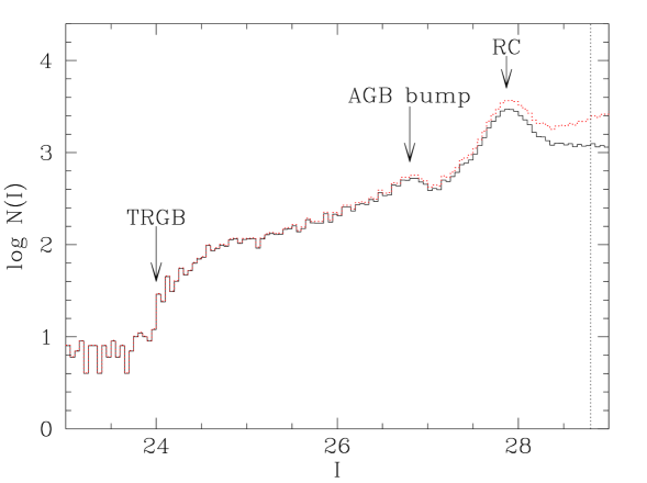
Figure 16: The measured $I$-band luminosity function (not corrected for extinction) is plotted with (black) solid line, while the (red) dotted curve shows the completeness corrected luminosity function. The vertical dotted line indicates 50% completeness magnitude of $I=28.80$. The main features are indicated by arrows: tip of the RGB (TRGB) at $I_{0}\sim 24.0$, AGB bump at $I_{0}\sim 26.77$ and red clump (RC) at $I_{0}\sim 27.87$.

The $I$-band luminosity function of the observed halo field is in Table 3 and is shown in Figure 16. The measured $I$-band luminosity function (not corrected for extinction) is plotted as the black solid line, while the (red) dotted curve shows the completeness corrected luminosity function. The vertical dotted line indicates 50% completeness magnitude of $I=28.80$. The main features are indicated by arrows: the RGB tip, the AGB bump, and the red clump.

6.1 Comparison with the M32 luminosity function

The nearest example of an elliptical galaxy is M32. Spectroscopically it is similar to faint ellipticals, but its very high surface brightness and proximity to M31 make it somewhat of an unusual case and a very difficult object to study. Grillmair et al. (1996) presented its $VI$ CMD obtained with WFPC2 on HST, which appears very similar to the CMD of our field in NGC 5128. The comparison of the luminosity function in NGC 5128 and in M32 is presented in Figure 17, where the latter was scaled using the distance modulus of $(m-M)^{M32}=24.43$ and reddening of $E_{B-V}^{M32}=0.08$. The scaling of the number counts was chosen arbitrarily.

The RGB tip and the RC features have very similar luminosities in the two galaxies, implying similar ages if the metallicity distributions are the same. However, according to Grillmair et al. (1996) the M32 population may be more metal-rich than the halo population in NGC 5128. It should be noted though that the observations of M32 sampled the inner $1^{\prime}-2^{\prime}$, which may well have higher metallicity than its outer regions. The absence of the AGB bump feature in the M32 luminosity function is most probably due to larger photometric errors and larger magnitude bins along the luminosity function.

6.2 RGB tip

The RGB tip, the feature due to the helium flash luminosity, is often used as a “standard candle” to determine galaxy distances. Its brightness in the I-band is (almost) independent of age and metallicity for metal-poor ($\mathrm{[Fe/H]}\leq-0.7$ dex), hence blue RGB stars (Da Costa & Armandroff, 1990; Harris et al., 1999). Selecting only blue stars in our CMD ($(V-I)<1.8$) we use a Sobel filter (see Lee et al., 1993) to measure the RGB tip magnitude. The filter is applied to luminosity functions computed with various bin sizes, ranging from 0.015 to 0.025 with a step of 0.005, each yielding one measurement of the RGB tip magnitude. The average of all these measurements is $I(TRGB)=24.05\pm 0.05$. This is in agreement with the estimate of $24.1\pm 0.1$ from the 21-kpc field (Harris et al., 1999) and $24.0\pm 0.1$ as measured by Soria et al. (1996) for a 10-kpc field.

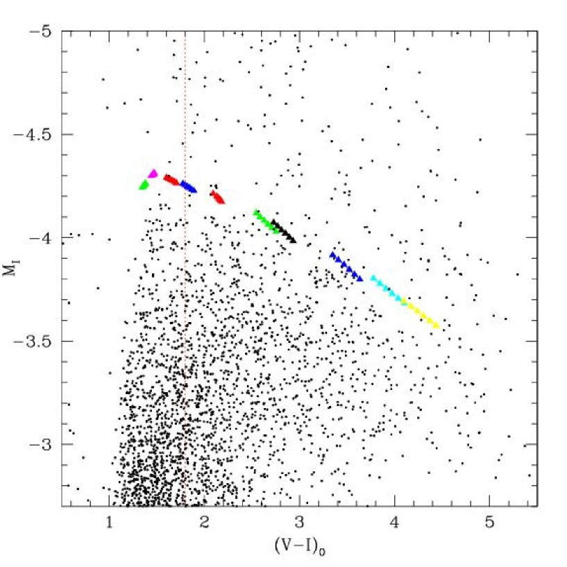
Figure 18: The comparison between the observed $VI$ CMD and the RGB tip magnitude as a function of age and metallicity. The RGB tip magnitude predictions from Pietrinferni et al. (2004) stellar evolutionary models are plotted as (colored) triangles for 10 different metallicities (Z=0.0001, 0.0003, 0.001, 0.002, 0.004, 0.008, 0.01, 0.0198, 0.03 and 0.04) and ages ranging from 7 to 12 Gy. Models of different ages for a fixed metallicity are connected with lines (see electronic edition for the color version of this figure).

Our data provide an excellent opportunity to check the dependence of the RGB tip magnitude on metallicity in the models. With respect to globular clusters, this dataset has the following advantages: (1) very good sampling of the RGB tip (where evolutionary lifetimes are short); (2) wide range of metallicity; and (3) same distance. The obvious disadvantage is the fact that the stars at RGB tip in our field have a range of ages and metallicities and the models predict some dependence of RGB tip I-band magnitude on star-formation history and in particular on the age-metallicity relation (Salaris & Girardi, 2005). The comparison of the model predictions for the RGB tip magnitudes in the range of ages between $7\leq age\leq 12$ Gy and for 10 different heavy metal abundances (Z=0.0001, 0.0003, 0.001, 0.002, 0.004, 0.008, 0.01, 0.0198, 0.03 and 0.04), computed using stellar evolutionary tracks of Pietrinferni et al. (2004), is shown in Figure 18. The triangles of different colors connected with lines (see the electronic version for the color figure) show RGB tip magnitudes for models of fixed metallicity and ages between 7 and 12 Gy. The RGB tip $I$-band magnitude is fainter for older ages at a fixed metallicity. The vertical dotted line is drawn at $V-I=1.8$, the reddest color for the measurement of the RGB tip magnitude. These models reproduce well the slope of I magnitude which gets fainter as V-I gets redder or the stars more metal-rich. However, they predict a brighter RGB tip magnitude than observed by $\sim 0.2$ mag. We believe it is largely due to the adopted $\mathrm{BC}_{I}$ scale (see detailed discussion in Salaris & Girardi, 2005). Part of the difference may also come from the combined uncertainty of the RGB tip magnitude measurement ($I^{TRGB}$) from the data and the uncertainty in the adopted distance modulus of NGC 5128 (Harris et al., 1999; Rejkuba, 2004), which is of the order of 0.15 mag.

6.3 AGB bump

The AGB bump feature is related to the evolutionary behavior of stellar models when helium is exhausted in the core and ignited in a shell. As the central helium burning approaches the end, the core contracts rapidly, until a helium burning shell is ignited. The ensuing violent expansion pushes the star temporarily out of thermal equilibrium and the model climbs rapidly to brighter luminosities (Renzini, 1977). When the helium shell is fully ignited, thermal equilibrium is restored in the stellar envelope and evolution proceeds on a nuclear timescale. This marks the base of the slow evolution on the AGB, or the AGB bump. Due to the very short lifetime of the AGB phase, the AGB bump feature can be detected only when dealing with large samples of stars. From the observational point of view it was discussed by Gallart (1998) and Ferraro et al. (1999). Alves & Sarajedini (1999) and Cassisi et al. (2001) have discussed theoretical predictions for AGB bump magnitude as a function of age and metallicity of the parent population.

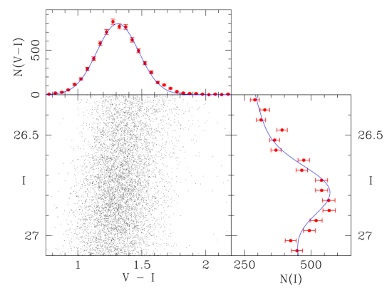
Figure 19: A zoom on the CMD around the AGB bump feature. On the right the I-band luminosity function around the AGB bump is fitted with a Gaussian plus a straight line. The peak is at $I=26.77\pm 0.01$ and $\sigma=0.12$. Above we show a Gaussian fit to the color distribution around the AGB bump.

The bump in the $I$-band luminosity function in Figure 16 around $I\sim 26.8$ occurs at the right magnitude expected for an AGB bump. At this level our photometry is $\sim 90$% complete. A linear relation plus a Gaussian provides a good fit to the I-band luminosity function in the range $26<I<27.1$ (Fig. 19). The best-fit Gaussian has the following parameters: mean magnitude, corresponding to the observed magnitude of the AGB bump, is $I=26.77\pm 0.01$, corresponding to $M_{I}^{AGBb}=-1.31$, and the standard deviation is 0.12 mag. The mean color of the AGB bump is $V-I=1.313\pm 0.003$ with a width of the Gaussian fit of 0.166 mag. The mean magnitude and color errors in this region of the CMD are of the order of 0.085 mag.

The appreciable color range present in the AGB clump smears out this feature in the V-band luminosity function. Still, a small bump is observed also in $V$ and the best fitting Gaussian plus a straight line give $V=27.97\pm 0.07$, corresponding to $M_{V}^{AGBb}=-0.29$, and $\sigma=0.13$. The somewhat wider AGB bump in $V$ is the consequence of the higher sensitivity on metallicity of this feature in the $V$ band, rather than in the $I$ band (see below) and of the wide metallicity distribution of stars contributing to the feature. It is not obvious how much a possible age spread in the halo also widens the bump. A more complete analysis will be done later through simulations of the entire CMD. Here we compare the mean magnitude and color of the AGB bump and the red clump (see next section) to stellar models in order to determine a plausible mean age of the halo stars.

6.4 Red clump

From the MDF, and from the absence of defined blue horizontal branch, it can be concluded that the metal-poor component is virtually absent in this galaxy, even in the outermost halo. On contrary, in M31 halo, which has been shown to have significant intermediate-age as well as metal-rich component (Durrell et al., 2004; Brown et al., 2003), blue horizontal branch is well defined and extends $\sim 1$ mag bluer than the average red giant branch color. In NGC 5128, most of the core helium burning stars are located in the red clump (RC) attached to the RGB sequence. A Gaussian plus a straight line again provides a good fit to the I-band luminosity function here as well, in the range $27.2<I<29$ (Fig. 20). The best fit Gaussian has a mean magnitude, corresponding to the observed magnitude of the RC, of $I(RC)=27.873\pm 0.002$ (corresponding to $M_{I}^{RC}=-0.21$) with $\sigma=0.18$. The mean color of the RC is $V-I=1.126\pm 0.001$ with a spread of $0.23$. The mean magnitude and color errors in this region of the CMD are 0.18 and 0.2 mag. Thus a large part of the width of the RC is due to photometric errors and not only due to a mix of populations. The completeness level of the photometry varies across the RC magnitudes between 50% and 75% (Fig. 20).

In the $V$-band the luminosity function of the RC can be fitted with a Gaussian at $V=28.951\pm 0.003$ and with $\sigma=0.20$. This corresponds to $M_{V}^{RC}=0.69$ mag.

7 Comparison with models

In this section we compare the magnitudes of the AGB bump and the RC features with the most recent stellar evolutionary tracks from Pietrinferni et al. (2004), in order to derive the mean age for the halo stars in our field. It is obvious from the upper RGB, as well as from the previous work, that there is a wide range of metallicities present in the field; but some age spread cannot be excluded (Rejkuba et al., 2003; Peng et al., 2004b). Therefore we need to map the theoretical location of the AGB bump and the Red Clump for populations in a range of age and metallicity. To do that we construct theoretical luminosity functions of Simple Stellar Populations (i.e. assembly of stars with the same age and metallicity, SSP) as follows.

For an SSP, the number of stars in any magnitude bin (j) along the post main sequence (MS) portion of its representative isochrone can be approximated fairly well by:

$$\Delta N_{j}^{SSP}=\phi(M_{TO})|\dot{M}_{TO}|\Delta t_{j}$$ (9)

where $M_{TO}$ is the turn-off mass of the isochrone, $\dot{M}_{TO}$ is the rate of change of $M_{TO}$ for increasing age of the isochrone, $\phi(M_{TO})$ is the initial mass function (IMF) evaluated at the turn-off mass, and $\Delta t_{j}$ is the evolutionary lifetime spent by $M_{TO}$ within the j-th magnitude bin (Renzini, 1981). This equation follows from approximating the post MS section of the isochrone with the evolutionary track with mass equal to $M_{TO}$.

Adopting, as usual, $\phi(M)\propto M^{-\alpha}$, Eq. 9 can be written as (Greggio, 2002):

$$\Delta N_{j}^{SSP}=M^{SSP}\beta_{\alpha}\Delta t_{j}$$ (10)

where $M^{SSP}$ is the total stellar mass of the SSP and $\beta_{\alpha}$ is the evolutionary flux at the turn-off per unit mass (i.e. number of stars leaving the MS per unit time in a SSP of 1 $M_{\odot}$):

$$\beta_{\alpha}=f_{\alpha}M_{TO}^{-\alpha}|\dot{M}_{TO}|.$$ (11)

In this equation $f_{\alpha}$ is a factor which depends only on the IMF, while both $\beta_{\alpha}$ and $\Delta t_{j}$ depend on age and metallicity.

Using this formalism it is possible to construct theoretical luminosity functions for the post MS phases of SSPs from a set of stellar tracks. We have considered Pietrinferni et al. (2004) evolutionary models for masses $\leq 2.5~{}M_{\odot}$ and the available heavy element abundances (i.e. Z=0.0001, 0.0003, 0.001, 0.002, 0.004, 0.008, 0.01, 0.0198, 0.03 and 0.04). These models were computed using a scaled solar distribution for the heavy elements and the solar model has $Z=0.0198$ and $Y=0.273$ (see Pietrinferni et al., 2004, for details). The turn-off ages of these models range between $0.4\lesssim\tau\lesssim 17$ Gy. For each chemical composition we have constructed the relation between turn-off mass and age ($\tau$) which turned out to be well represented by a parabola on the $\log M-\log\tau$ plane. We have thus obtained the analytic $\beta_{\alpha}$ functions for the various chemical compositions. The luminosity function of an SSP of unitary mass is then computed as $\Delta n_{j}^{SSP}=\beta_{\alpha}\Delta t_{j}$, in which the quantities $\Delta t_{j}$ are read from the track whose evolutionary lifetime is equal to the age of the SSP.

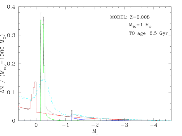
Figure 21: Comparison between the observed luminosity function (dashed cyan line) and the luminosity function predicted for an age of 8.5 Gy and heavy element abundance of $Z=0.008$, computed with the evolutionary tracks of Pietrinferni et al. (2004). We plot separately the RGB (red), core helium burning (green) and AGB luminosity functions (blue). The sum of these three components is plotted with the dotted (black) line. This theoretical LF predicts $M_{I}(AGBb)\simeq-1.2$, $M_{I}(RC)\simeq-0.8$, and $M_{I}(RGBbump)\simeq 0.1$ mag. From this comparison it is apparent that the RC feature has most probably also a contribution from RGB bump (RGBbump) stars. (see electronic edition for the color version of this figure)

Figure 21 shows one such example of a theoretical luminosity function for an age of 8.5 Gy and heavy element abundance of $Z=0.008$. We plot separately the RGB (red), helium burning (green), and AGB portions (blue), as well as the total luminosity function (black dotted line). The (cyan) dashed line shows our observed, completeness corrected luminosity function, scaled between $-2<M_{I}<-2.5$ to match the theoretical luminosity function (in this particular case the adopted scaling factor is 25321). The width of the observed Red Clump feature is partly due to photometric errors, and partly reflects the age and metallicity spread. In addition, the comparison between the data and the models indicates that the RC has most probably also a contribution from the RGB bump feature. However, since the expected number of stars in the RGB bump is relatively small compared to that in the RC, we neglect its effect on the magnitude location of the Red Clump.

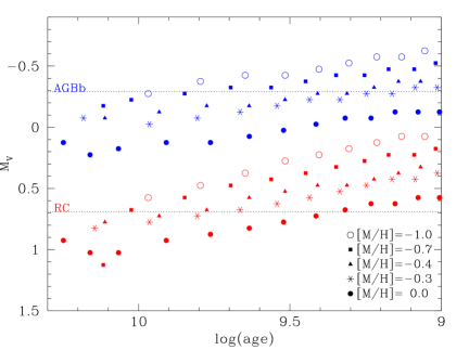
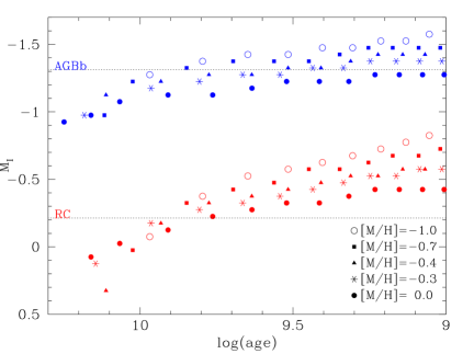
Figure 22: $V$ (top) and $I$ (bottom) magnitudes of AGB bump and red clump features predicted by the models are plotted as a function of age for 5 metallicities, covering most of the range of observed MDF in the halo of NGC 5128. For comparison the observed AGB bump and RC magnitudes are indicated with horizontal dotted lines.

Figure 22 shows the comparison between the measured $V$ (top panel) and $I$ magnitudes (bottom panel) of AGB bump and RC features in NGC 5128 halo with models of five different metallicities plotted as a function of age. The model $M_{I}$ and $M_{V}$ values are the peak magnitudes obtained from the theoretical luminosity functions described above. The $V$ band has a greater sensitivity to metallicity, but the age sensitivity is similar for both bands. It is thus useful to compare the values coming from observations in both bands. However, it should be kept in mind that the AGB bump magnitude has much larger uncertainty, in particular in the $V$ band. We can derive a first estimate of the mean age of the stellar population in our field by considering that its average metallicity is $\mathrm{[M/H]}=-0.6$ dex, which is close to that of the models represented as filled squares. The location of both features in both bands indicates an average age around 8 Gy.

A better estimate of the average age of the stars in our field can be obtained by computing the average magnitude of the RC and of the AGB bump expected for the metallicity distribution determined from our data:

$$\langle Mag(age)\rangle=\int_{\Delta Z}N(Z)Mag(Z,age)dZ$$ (12)

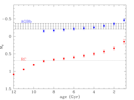
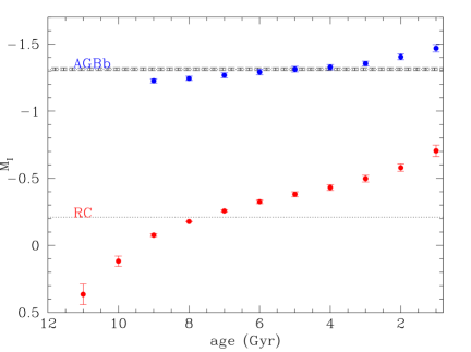
Figure 23: Average $V$ (top) and $I$ (bottom) magnitudes of AGB bump and red clump features predicted by the models, obtained by convolving the metallicity dependency with the measured metallicity distribution of the RGB halo stars (see Eq. 12), are plotted as a function of age. The measured AGB bump (AGBb) and RC magnitudes are shown as dotted horizontal lines. We also plot $1\sigma$ error-bars for the uncertainty in the AGB bump mean magnitude fit. The error-bars on the model points are calculated from assumed $\pm 0.1$ dex uncertainty in the measured metallicity distribution.

This estimate will be adequate insofar the age spread is small, and as long as our derived metallicity distribution does not depend strongly on age. As we argued earlier this is the case for the ages of 8 Gy and older. Figure 23 shows the comparison between the observed AGB bump and RC magnitude, and the results of the application of Eq. 12 at various ages. The $1\sigma$ uncertainty in the measured AGB bump magnitude is indicated with shaded stripes, while the measurement of the mean RC magnitude has negligible errors due to much larger number of stars and is thus shown as a horizontal line. It should be kept in mind that this is only the statistical error-bar for the measurement of the mean RC and AGB bump magnitude in our data, but it does not include systematic errors due to reddening and distance uncertainties, which are of the order of $\pm 0.15$ mag. The error-bars of the model data points are calculated by using the Eq. 12 with $\pm 0.1$ dex shift in the observed metallicity distribution and they do not include any uncertainty due to the adopted bolometric corrections or uncertainties in the models themselves, which are particularly relevant for the AGB phase (Cassisi et al., 2001).

For metal-poor populations with $\mathrm{age}>9$ Gy, the AGB bump feature is not visible in the theoretical luminosity functions, and there is only a very weak feature present for more metal-rich and old stars. Thus we do not plot the model predictions for mean magnitudes of the AGB bump for older ages.

The $V$ band magnitude of the RC favors an average age for the halo stars of 8.5 Gy, while the $I$ band measurement agrees better with an average age of $7.6$ Gy. As shown above the $V$ band is more sensitive to metallicity than the $I$-band. Thus even small errors in the metallicity distribution (due to inclusion of AGB giants, or due to interpolation with tracks that have different age than the true distribution) can have large effect on the $V$-band models. This can be also appreciated by the size of the error-bars on the model points. The AGB bump magnitudes in both bands seem to favor slightly younger ages, but the shallower dependence of the AGBb with age and its larger internal uncertainty do not exclude the average age of $8^{+2}_{-2.5}$ Gy, where the error-bars include $0.15$ mag uncertainty in the reddening and distance modulus.

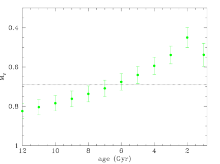
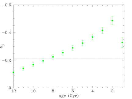
Figure 24: Average $V$ (top) and $I$ (bottom) magnitudes of red clump predicted by the models of Girardi et al. (2000); Girardi & Salaris (2001), obtained by convolving the metallicity dependency with the measured metallicity distribution of the RGB halo stars (see Eq. 12), are plotted as a function of age. The measured RC magnitudes are shown as dotted horizontal lines. The error-bars on the model points are calculated from assumed $\pm 0.1$ dex uncertainty in the measured metallicity distribution.

We note that even though there is a rather large discrepancy between the observed tip of the RGB and that predicted by the models of Pietrinferni et al. (2004), this is most probably largely due to uncertain bolometric corrections for these cool giants (see sect. 6.2). The uncertainty in bolometric corrections for AGB bump and RC evolutionary phases is expected to be much smaller. In order to test the uncertainty due to adoption of the particular set of models we also compare the observed magnitude of the RC in our field with another set of model predictions, using the results published by Girardi & Salaris (2001), which are based on Padova group models (Girardi et al., 2000). The average metallicity weighted RC magnitude as a function of age (points in Fig. 24) was calculated again using the Eq. 12. Figure 24 shows the result. As before, the error bars on the model data points show the effect of 0.1 dex shift in the observed MDF and the dotted horizontal line indicates the measured magnitude of the red clump. Contrary to the models of Pietrinferni et al. (2004), the $V$-band magnitude of the RC indicates younger average age of 6.5 Gy, while the $I$-band magnitude would imply 8.5 Gy for the average age of the halo stars. The difference in age predicted in the two photometric bands for Padova models (Girardi et al., 2000) is almost twice as large as that for Teramo models (Pietrinferni et al., 2004), and we add 1 Gy error due to that. However, this does not change our conclusion about the average age of $8^{+3}_{-3.5}$ Gy for the halo stars in NGC 5128.

8 Conclusions and summary

We present a very deep CMD of a remote halo field in NGC 5128, located 38 kpc south from the center of the galaxy. The high resolution and sensitivity of the ACS WFC instrument at HST allowed us for the first time to detect the AGB bump and RC features in a E/S0 galaxy. From the colors of RGB stars we derive the metallicity distribution, assuming no age dependency (and an old age) of the models.

The metallicity distribution is broad and moderately rich with average $\mathrm{[M/H]}=-0.64$ dex and a $1\sigma$ spread of $0.49$ dex. It is very similar to the MDFs derived from earlier observations of 21 and 31 kpc fields, except for a slightly larger number of most metal-rich stars, which were missed in the previous observations. This metallicity distribution is convolved with the models for AGB bump and RC magnitudes which are dependent both on age and metallicity to derive an average age of $\sim 8^{+3}_{-3.5}$ Gy for the halo stars.

In the models with ages $\gtrsim 10$ Gy there are very few AGB bump stars compared to the RC or horizontal branch. In metal-poor ($\mathrm{[M/H]}<-1$ dex) and old ($\mathrm{age}>9$ Gy) models the AGB bump is not present at all, although (Ferraro et al., 1999) report the observations of an AGB bump for 4 Galactic globular clusters with $\mathrm{[M/H]}<-1$. Thus an alternate interpretation could be that a part of the population is “old” ($\gtrsim 10$ Gy) and that the AGB bump feature appears due to a second major star-burst event that happened $\sim 5-7$ Gy ago. The presence of these younger stars would brighten the average magnitude of the RC (Salaris et al., 2003), which would thus appear as a feature with a mean age around 8 Gy. This would be in agreement with some previous studies of NGC 5128 halo stars which suggested a 10% of intermediate-age stars (Soria et al., 1996; Marleau et al., 2000; Rejkuba et al., 2003). In a following paper we will investigate how much spread in age might be present in the halo stars through the simulations of the complete CMD. This will also allow us to derive a more accurate and internally consistent MDF and to account for the effect of photometric errors as well as the presence of some probable RGB bump contribution to the average magnitude of the RC.

Table 1: List of all the matched sources in ACS and EMMI images that passed visual inspection and were used to derive calibration Equations 5 and 7.

ACS EMMI x y F606W $\sigma_{F606W}$ F814W $\sigma_{F814W}$ x y V $\sigma_{V}$ I $\sigma_{I}$ pix pix mag mag mag mag pix pix mag mag mag mag 3937.97 154.85 21.330 0.017 20.404 0.022 328.96 397.22 21.590 0.012 1.312 0.030 2164.61 192.27 21.508 0.009 19.435 0.015 292.14 659.77 22.085 0.018 2.570 0.021 3615.89 279.24 20.772 0.012 19.806 0.014 339.63 447.76 21.152 0.011 1.215 0.017 3719.73 402.83 21.804 0.012 20.417 0.014 360.29 435.40 22.268 0.018 1.770 0.027 1572.44 410.62 23.330 0.010 21.142 0.010 310.11 752.41 23.967 0.076 2.732 0.086 2776.76 420.25 22.374 0.006 20.443 0.011 340.30 574.91 22.968 0.025 2.446 0.032 3218.67 448.54 21.487 0.012 19.497 0.018 355.10 510.42 22.043 0.018 2.515 0.021 3155.36 638.67 21.917 0.014 19.854 0.019 381.67 524.34 22.434 0.025 2.586 0.028 3283.54 720.19 21.309 0.010 20.485 0.014 396.71 507.44 21.618 0.009 1.042 0.020 3996.31 796.90 22.468 0.018 21.098 0.021 425.07 404.14 22.882 0.028 1.820 0.040 57.28 812.82 21.609 0.018 20.335 0.019 333.09 985.33 22.055 0.016 1.652 0.023 3267.80 852.76 22.679 0.010 21.798 0.011 415.80 513.06 23.000 0.034 1.051 0.070 325.51 950.30 21.622 0.009 20.640 0.011 359.85 949.15 22.058 0.018 1.263 0.027 345.39 1028.98 21.201 0.008 19.729 0.010 371.94 948.10 21.763 0.015 1.970 0.019 191.73 1060.88 23.073 0.019 21.415 0.017 372.84 971.47 23.640 0.071 2.204 0.085 1542.83 1067.58 22.706 0.017 21.575 0.016 406.35 772.59 23.151 0.041 1.522 0.058 1335.47 1218.15 21.641 0.021 19.999 0.020 423.49 806.74 22.135 0.013 2.151 0.019 233.39 1392.28 21.862 0.013 20.944 0.015 422.82 973.32 22.187 0.016 1.172 0.031 702.78 1682.18 21.689 0.009 20.389 0.010 476.78 911.16 22.215 0.022 1.743 0.031 734.77 1813.78 20.804 0.009 19.835 0.010 496.92 909.57 21.152 0.009 1.176 0.016 296.15 1833.29 22.180 0.012 19.935 0.011 489.35 974.68 22.831 0.028 2.881 0.032 1093.76 1998.74 23.232 0.007 21.427 0.009 532.81 861.25 23.819 0.069 2.260 0.087 3077.80 2333.91 21.175 0.010 19.471 0.021 629.62 577.00 21.756 0.013 2.275 0.016 137.91 2434.48 22.074 0.018 21.470 0.015 574.10 1012.42 22.079 0.029 0.968 0.065 2877.56 2481.52 21.177 0.016 19.376 0.025 646.58 610.11 21.790 0.013 2.458 0.015 2415.01 2489.81 21.095 0.014 20.436 0.019 636.80 678.41 21.391 0.010 0.861 0.019 1053.66 2514.91 22.620 0.012 22.000 0.011 607.97 879.62 22.342 0.026 0.741 0.061 2985.42 2632.81 20.519 0.017 19.348 0.020 671.49 597.82 20.891 0.008 1.443 0.012 3739.75 2644.34 21.703 0.014 20.755 0.019 691.16 486.85 22.119 0.016 1.293 0.027 2296.51 2698.13 20.280 0.015 18.652 0.028 664.63 700.93 20.853 0.009 2.068 0.013 3216.61 2721.97 21.870 0.010 21.008 0.010 690.23 565.81 21.594 0.012 0.869 0.026 976.82 2729.66 20.458 0.013 19.653 0.013 637.81 896.15 20.722 0.007 0.991 0.012 1405.38 2776.88 20.550 0.011 19.728 0.011 655.03 834.17 20.878 0.009 1.026 0.014

Table 1: continue.

ACS EMMI x y F606W $\sigma_{F606W}$ F814W $\sigma_{F814W}$ x y V $\sigma_{V}$ I $\sigma_{I}$ pix pix mag mag mag mag pix pix mag mag mag mag 3754.16 2792.53 23.679 0.009 21.546 0.011 713.44 488.34 24.208 0.095 2.602 0.110 2596.22 2905.00 20.710 0.014 20.039 0.013 702.33 661.71 20.928 0.009 0.876 0.016 3608.48 2973.34 21.595 0.008 20.183 0.011 736.49 514.14 22.131 0.016 1.862 0.025 3252.45 2993.42 21.880 0.017 20.510 0.018 731.08 567.09 22.313 0.030 1.860 0.042 1917.10 3038.22 23.202 0.017 20.978 0.019 705.74 765.06 23.884 0.060 2.792 0.068 3762.43 3039.05 20.480 0.013 19.623 0.014 749.87 492.95 20.803 0.007 1.170 0.012 3714.12 3048.16 20.550 0.014 19.788 0.015 750.05 500.30 20.760 0.006 0.908 0.011 2247.26 3075.96 22.896 0.012 20.762 0.012 719.11 717.31 23.511 0.047 2.710 0.055 2152.90 3102.38 20.842 0.011 20.084 0.019 720.78 731.80 21.116 0.011 0.907 0.021 557.92 3117.79 22.646 0.014 20.694 0.015 684.85 967.12 23.405 0.050 2.579 0.057 2906.24 3133.20 20.304 0.017 19.455 0.019 743.31 621.48 20.565 0.005 1.033 0.011 1693.17 3170.59 21.351 0.017 20.280 0.019 719.84 801.17 21.793 0.012 1.404 0.021 3829.93 3249.78 22.354 0.013 20.255 0.013 782.62 488.05 22.956 0.032 2.721 0.037 2369.70 3261.08 23.113 0.020 22.367 0.020 749.36 703.61 23.395 0.055 0.754 0.129 2314.35 3275.75 20.546 0.012 19.738 0.014 750.18 712.14 20.852 0.007 1.003 0.012 3169.78 3277.28 21.489 0.016 20.577 0.017 770.82 586.10 21.832 0.021 1.179 0.034 1772.95 3410.03 22.544 0.014 21.649 0.014 756.90 795.12 22.838 0.031 1.106 0.060 1942.42 3436.93 22.119 0.017 20.199 0.015 764.96 770.82 22.763 0.031 2.556 0.039 1571.33 3439.63 22.400 0.016 20.925 0.016 756.49 825.59 22.902 0.031 1.929 0.042 1970.27 3511.46 19.634 0.025 18.865 0.025 776.71 768.51 19.869 0.005 0.823 0.009 2059.34 3555.50 20.410 0.014 19.397 0.014 785.26 756.44 20.840 0.007 1.328 0.012 1586.23 3573.68 22.616 0.013 20.849 0.012 776.70 826.61 23.225 0.045 2.297 0.052 3558.91 3613.37 22.513 0.010 22.417 0.016 829.65 536.79 22.586 0.021 0.282 0.086 3498.78 3687.52 20.827 0.010 19.348 0.025 839.05 547.34 21.322 0.009 1.968 0.013 2483.60 3769.17 21.306 0.014 19.866 0.012 826.89 698.98 21.841 0.013 1.936 0.019 3942.52 3787.70 22.105 0.009 21.235 0.011 864.41 484.30 22.474 0.023 1.332 0.038 2806.78 3843.25 20.498 0.016 19.556 0.019 845.49 653.14 20.816 0.007 1.230 0.014 2673.56 4046.14 21.995 0.014 20.015 0.013 872.12 677.60 22.667 0.024 2.625 0.029 3180.09 4101.70 20.500 0.018 19.677 0.022 892.49 604.25 20.806 0.006 1.116 0.011 918.68 1230.76 19.951 0.024 18.485 0.028 415.36 868.50 20.510 0.006 1.971 0.008 2188.31 2811.40 20.267 0.017 19.097 0.023 678.75 719.58 20.740 0.007 1.582 0.012 2116.95 2905.26 20.215 0.016 19.447 0.017 690.93 732.34 20.411 0.007 0.911 0.012 3552.66 3237.15 20.936 0.010 19.359 0.020 774.04 528.65 21.477 0.010 2.129 0.013 1786.06 105.93 19.860 0.019 18.797 0.028 270.33 713.50 20.317 0.006 1.260 0.009

Table 2: Average metallicities and spread in [M/H] measured for the NGC 5128 halo stars at various distances from the center.

Distance $\langle$[M/H]$\rangle$ $\sigma$ (kpc) (dex) (dex) 8 $-0.46$ $0.48$ 21 - 31 $-0.69$ $0.49$ 38 $-0.65$ $0.49$

Table 3: Observed I-band luminosity function of NGC 5128 halo stars 38 kpc away from the center of the galaxy. $I$ is the magnitude of the bin center, $N$ are the raw counts in a given magnitude bin and $N_{corr}$ are completeness corrected counts.

I N N_corr I N N_corr I N N_corr I N N_corr I N N_corr 22.62 6 6 23.88 10 10 25.12 92 94 26.38 309 326 27.62 1451 1706 22.67 8 8 23.92 9 9 25.17 115 118 26.42 295 312 27.67 1855 2200 22.73 7 7 23.98 12 12 25.22 128 131 26.47 369 391 27.72 2176 2606 22.77 4 4 24.02 29 29 25.27 132 136 26.52 342 363 27.77 2467 2986 22.82 11 11 24.07 24 24 25.32 129 133 26.57 346 368 27.82 2840 3476 22.88 6 6 24.12 45 46 25.38 130 134 26.62 443 473 27.88 2964 3672 22.92 7 7 24.17 31 32 25.42 147 151 26.67 435 465 27.92 2933 3681 22.98 1 1 24.23 40 41 25.47 149 154 26.72 503 539 27.97 2811 3577 23.02 8 8 24.27 55 56 25.52 160 165 26.77 502 540 28.02 2517 3251 23.07 6 6 24.32 47 48 25.57 138 143 26.82 525 566 28.07 2270 2979 23.12 7 7 24.38 52 53 25.62 150 155 26.88 525 568 28.12 2006 2679 23.17 9 9 24.42 63 64 25.67 187 194 26.92 478 519 28.17 1661 2259 23.23 4 4 24.48 70 71 25.72 173 179 26.97 453 494 28.22 1492 2070 23.27 8 8 24.52 73 74 25.77 172 178 27.02 387 423 28.27 1475 2091 23.32 8 8 24.57 98 100 25.82 172 179 27.07 407 447 28.32 1348 1955 23.38 4 4 24.62 86 88 25.88 217 226 27.12 395 436 28.38 1207 1793 23.42 8 8 24.67 91 93 25.92 176 183 27.17 504 559 28.42 1272 1940 23.48 6 6 24.73 99 101 25.97 214 223 27.22 487 543 28.47 1263 1980 23.52 9 9 24.77 96 98 26.02 206 215 27.27 549 615 28.52 1211 1955 23.57 6 6 24.82 113 116 26.07 256 267 27.32 610 687 28.57 1252 2085 23.62 8 8 24.88 115 118 26.12 256 268 27.38 739 837 28.62 1158 1993 23.67 4 4 24.92 103 105 26.17 233 244 27.42 770 878 28.67 1226 2185 23.73 7 7 24.98 114 117 26.22 272 286 27.47 830 953 28.72 1178 2178 23.77 10 10 25.02 115 118 26.27 278 292 27.52 965 1116 28.77 1190 2286 23.82 11 11 25.07 116 119 26.32 274 289 27.57 1194 1392 28.82 1250 2500

Figure 12: The distribution of $V-I$ color in different magnitude bins along the RGB.

Figure 17: The comparison between the LFs of NGC 5128 derived here (solid line) and M32 LF from Grillmair et al. (1996) (dashed line).

Figure 20: A zoom on the CMD around the red clump feature. On the right the I-band luminosity function around the RC is fitted with a Gaussian plus a straight line. The peak is at $I=27.873\pm 0.002$ and $\sigma=0.18$. Above we show a Gaussian fit to the color distribution.

References

- Alves & Sarajedini (1999) Alves, D. R. & Sarajedini, A., 1999, ApJ, 511, 225
- Ashman & Zepf (1992) Ashman, K. M. & Zepf, S. E., 1992, ApJ, 384, 50
- Bahcall & Soneira (1981) Bahcall, J. N., & Soneira, R. M., 1981, ApJS, 47, 357
- Beasley et al. (2003) Beasley, M. A., Harris, W. E., Harris, G. L. H. & Forbes, D. A., 2003, MNRAS, 340, 341
- Bedin et al. (2005) Bedin, L. R., Cassisi, S., Castelli, F., et al., 2005, MNRAS in press, astro-ph/0412328
- Bergbusch & VandenBerg (2001) Bergbusch, P. A., & VandenBerg, D. A. 2001, ApJ, 556, 322
- Brown et al. (2003) Brown, T. M., Ferguson, H. C., Smith, E., et al. 2003, ApJ, L17
- Burstein & Heiles (1982) Burstein, D. & Heiles, C., 1982, AJ, 87, 1165
- Cardelli et al. (1989) Cardelli, J. A., Clayton, G. C. & Mathis, J. S., 1989, ApJ, 345, 245
- Cassisi et al. (2001) Cassisi, S., Castellani, V., Degl’Innocenti, S., Piotto, G., & Salaris, M. 2001, A&A, 366, 578
- Cole et al. (2000) Cole, S., Lacey, C. G., Baugh, C. M. & Frenk, C. S., 2000, MNRAS, 319, 168
- Coté et al. (1998) Coté, P., Marzke, R. O. & West, M. J., 1998, ApJ, 501, 554
- Da Costa & Armandroff (1990) Da Costa, G. S. & Armandroff, T. E., 1990, AJ, 100, 160
- Davidge & van den Bergh (2001) Davidge, T. J. & van den Bergh, S., 2001, ApJ, L133
- Dekker et al. (1986) Dekker, H., Delabre, B. & D’Odorico, S., 1986, SPIE 627, 339
- Dressler et al. (2004) Dressler, A., Oemler, A., Jr., Poggianti, B. M., et al., 2004, ApJ, 617, 867
- Durrell et al. (2004) Durrell, P. R., Harris, W. E. & Pritchet, C. J., 2004, AJ, 128, 260
- Fassett & Graham (2000) Fassett, C.I. & Graham, J.A., 2000, ApJ, 538, 594
- Ferraro et al. (1999) Ferraro, F. R., Messineo, M., Fusi Pecci, F., de Palo, M. A., Straniero, O., Chieffi, A., & Limongi, M. 1999, AJ, 118, 1738
- Ford et al. (1998) Ford, H. C., et al., 1998, Proc. SPIE, 3356, 234
- Fleming et al. (1995) Fleming, D.E.B, Harris, W.E., Pritchet, C.J., & Hanes, D.A., 1995, AJ, 109, 1044
- Gallart (1998) Gallart, C., 1998, ApJ, 495, L43
- Girardi & Salaris (2001) Girardi, L. & Salaris, M., 2001, MNRAS, 323, 109
- Girardi et al. (2000) Girardi, L., Bressan, A., Bertelli, G. & Chiosi, C., 2000, A&AS, 141, 371
- Graham (1998) Graham, J.A., 1998, ApJ, 502, 245
- Graham & Fassett (2002) Graham, J. A. & Fassett, C. I., 2002, ApJ, 575, 712
- Greggio (2002) Greggio, L. 2002, ASP Conf. Ser. 274: Observed HR Diagrams and Stellar Evolution, 444
- Gregg et al. (2004) Gregg, M. D., Ferguson, H. C., Minniti, D., Tanvir, N. & Catchpole, R., 2004, AJ 147, 1441
- Grillmair et al. (1996) Grillmair, C.J., Lauer, T.R., Worthey, G., et al., 1996, AJ, 112, 1975
- Harris & Harris (2000) Harris, G. L. H. & Harris, W. E., 2000, AJ, 120, 2423
- Harris et al. (1999) Harris, G.L.H., Harris, W.E. & Poole, G.B., 1999, AJ, 117, 855
- Harris & Harris (2002) Harris, W. E. & Harris, G. L. H. 2002, AJ, 123, 3108
- Harris et al. (1995) Harris, W. E., Pritchet, C. J. & McClure, R. D., 1995, ApJ, 441, 120
- Kauffmann et al. (1993) Kauffmann, G., White, S. D. M., Guideroni, B., 1993, MNRAS, 264, 201
- Kuntschner et al. (2002) Kuntschner, H., Smith, R. J., Colles, M., et al., 2002, MNRAS, 337, 172
- Landolt (1992) Landolt, A.U., 1992, AJ 104, 340
- Larson (1974) Larson, R. B., 1974, MNRAS, 166, 385
- Lee et al. (1993) Lee, M. G., Freedman, W. L. & Madore, B. F., 1993, ApJ, 417, 553
- Marleau et al. (2000) Marleau, F. R., Graham,J. R., Liu, M. C. & Charlot, S., 2000, AJ, 120, 1779
- Malin et al. (1983) Malin, D.F., Quinn, P.J. & Graham, J.A., 1983, ApJ 272, L5
- Mould et al. (2000) Mould, J.R., Ridgewell, A., Gallagher, J.S. III et al., 2000, ApJ, 536, 266
- Partridge & Peebles (1967) Partridge, R. B. & Peebles, P. J. E., 1967, ApJ, 147, 868
- Peng et al. (2004a) Peng, E. W., Ford, H. C. & Freeman, K. C., 2004a, ApJ, 602, 685
- Peng et al. (2004b) Peng, E. W., Ford, H. C. & Freeman, K. C., 2004b, ApJ, 602, 705
- Pietrinferni et al. (2004) Pietrinferni, A., Cassisi, S., Salaris, M., & Castelli, F. 2004, ApJ, 612, 168
- Puzia et al. (2004) Puzia, T. H., Kissler-Patig, M., Thomas, D., et al., 2004, A&A, 415, 123
- Rejkuba (2004) Rejkuba, M., 2004, A&A, 413, 903
- Rejkuba et al. (2001) Rejkuba, M., Minniti, D., Silva, D.R. & Bedding, T., 2001, A&A, 379, 781
- Rejkuba et al. (2002) Rejkuba, M., Minniti, D., Courbin, F. & Silva, D. R. 2002, ApJ, 564, 688
- Rejkuba et al. (2003) Rejkuba, M., Minniti, D., Silva, D. R. & Bedding, T. R., 2003, A&A, 411, 351
- Rejkuba et al. (2004) Rejkuba, M., Greggio, L. & Zoccali, M., 2004, A&A, 415, 915
- Renzini (1977) Renzini, A. 1977, in: ”Advanced Stages in Stellar Evolution”, ed. P. Bouvier & A. Maeder (Geneva Observatory), p. 151
- Renzini (1981) Renzini, A. 1981, Colors and Populations of Galaxies, 87
- Robin et al. (1996) Robin, A. C., Haywood, M., Creze, M., Ojha, D. K. & Bienayme, O., 1996, A&A, 305, 125
- Romanowsky et al. (2003) Romanowsky, A. J., Douglas, N. G., Arnaboldi, M., et al., 2003, Science, 301, 1696
- Rosenberg et al. (2000) Rosenberg, A., Piotto, G., Saviane, I. & Aparicio, A., 2000, A&AS, 114, 5
- Salaris et al. (2003) Salaris, M., Percival, S. & Girardi, L., 2003, MNRAS, 345, 1030
- Salaris & Girardi (2005) Salaris, M. & Girardi, L., 2005, MNRAS 357, 669
- Saviane et al. (2000) Saviane, I., Rosenberg, A., Piotto, G. & Aparicio, A., 2000, A&A, 355, 966
- Schlegel et al. (1998) Schlegel, D.J., Finkbeiner, D.P. & Davis, M., 1998, ApJ, 500, 525
- Schulte-Ladbeck et al. (2003) Schulte-Ladbeck, R. E., Drozdovsky, I. O., Belfort, M. & Hopp, U., 2003, Ap&SS, 284, 909
- Soria et al. (1996) Soria, R., Mould, J.R., Watson, A.M., et al., 1996, ApJ 465, 79
- Stickel et al. (2004) Stickel, M., van der Hulst, J.M., van Gorkom, J.H., Schiminovich, D. & Carilli, C.L., 2004, A&A, 415, 95
- Stetson (2000) Stetson, P.B., 2000, PASP, 112, 925
- Stetson (1994) Stetson, P.B., 1994, PASP, 106, 250
- Stetson (1987) Stetson, P.B., 1987, PASP, 99, 191
- Tinsley (1972) Tinsley, B. M., 1972, ApJ, 178, 319
- Toomre (1977) Toomre, A., 1977, in Tinsley B. M., Larson R. B. eds, The Evolution of Galaxies and Stellar Populations. Yale Univ. Obs., New Haven, p. 401
- Trager et al. (2000) Trager, S. C., Faber, S. M., Worthey, G. & González, J. J., 2000, AJ, 119, 1645
- VandenBerg et al. (2000) VandenBerg, D. A., Swenson, F. J., Rogers, F. J., Iglesias, C. A., & Alexander, D. R., 2000, ApJ, 532, 430
- Walsh et al. (1999) Walsh, J. R., Walton, N. A., Jacoby, G. H. & Peletier, R. F., 1999, A&A, 346, 753
- Yi et al. (2004) Yi, S. K., Peng, E., Ford, H., Kaviraj, S. & Yoon, S.-J., 2004, MNRAS, 3498, 1493