The Shape-Alignment relation in $\Lambda$CDM Cosmic Structures

Abstract

In this paper we study the supercluster - cluster morphological properties using one of the largest ($2\times 512^{3}$ SPH+N-body simulations of large scale structure formation in a $\Lambda$CDM model, based on the publicly available code GADGET. We find that filamentary (prolate-like) shapes are the dominant supercluster and cluster dark matter halo morphological feature, in agreement with previous studies. However, the baryonic gas component of the clusters is predominantly spherical. We investigate the alignment between cluster halos (using either their DM or baryonic components) and their parent supercluster major-axis orientation, finding that clusters show such a preferential alignment. Combining the shape and the alignment statistics, we also find that the amplitude of supercluster - cluster alignment increases although weakly with supercluster filamentariness.

1 Introduction

The wealth of recent observational data has brought great progress in understanding the cosmic structure formation pattern. At the largest cosmic scales it is known that clusters of galaxies are not randomly distributed but tend to aggregate in even larger conglomerations, the so called superclusters (cf. Oort 1983; Bahcall 1988). The large sizes of superclusters ($\raise-3.0pt\hbox{\hbox to0.0pt{\hbox{$\sim$}\hss}\raise 4.0pt\hbox{$>$}\ }30\;h^{-1}$ Mpc) in conjunction with the amplitude of their member cluster peculiar velocities ($\sim$ 1000 km/sec) imply that superclusters constitute unvirialized density fluctuations which should reflect the initial conditions that gave rise to structure formation processes.

Observational and theoretical studies of the supercluster morphology and environment suggest that they are not spherical but instead their shapes are elongated (eg. Zeldovich, Einasto & Shandarin 1982; de Lapparent, Geller & Huchra 1991) with a prolate-like tendency (eg. Frenk et al. 1988; Plionis, Valdarnini & Jing 1992; Dubinski 1994; Einasto et al. 2001; Jing & Suto 2002; Diaferio et al. 2003; Sheth et al. 2003; Einasto et al. 2003; Shandarin, Sheth, Sahni 2004; Pandey & Bharadwaj 2005). Sathyaprakash, Sahni & Shandarin (1998), Basilakos, Plionis & Rowan-Robinson (2001), Kolokotronis, Basilakos & Plionis (2002), using either the IRAS galaxy distribution or the Abell/ACO clusters, gave attention to the cosmological inferences of supercluster shape statistics claiming that a low matter density flat cosmological model ($\Omega_{\rm m}=1-\Omega_{\Lambda}=0.3$) fits the large-scale observational results at a high significance level.

A variety of indications support the formation of clusters by hierarchical aggregation of smaller units along filamentary large-scale structures (eg. West 1994; Ostriker & Cen 1996 and references therein). Under this scenario dynamically young clusters will have a tendency to be aligned with neighboring structures, since the accretion of matter takes place along the large-scale filamentary structure within which the clusters form. Indeed, observational studies of structure orientations, which has a long history in cosmology, have found strong indications of various alignment effects. Bingelli (1982) was the first to find that the major axes of neighboring clusters of galaxies tend to point toward each other. On the other hand, Struble & Peebles (1985) have failed to measure a significant alignment signal (see also Flin 1987; Rhee & Katgert 1987; Ulmer, McMillan, & Kowalski 1989). However, in the last decade many authors have claimed that cluster formation processes are strongly connected to the supercluster network and thus generate measurable environmental effects, among which strong alignment effects observed in both observational and N-body data (eg. West 1994; Plionis 1994; West, Jones, & Forman 1995; van Haarlem, Frenk & White 1997; Colberg et al. 2000; Onuora & Thomas 2000; Chambers, Mellot & Miller 2002; Plionis & Basilakos 2002; Faltenbacher et al. 2002; Plionis et al. 2003; Bailin & Steinmetz 2004; Kasun & Evrard 2004; Pimbblet 2005; Hopkins, Bahcall & Bode 2005; Lee, Kang & Jing 2005; Faltenbacher et al. 2005).

Furthermore, Plionis (2002; 2004) using the APM galaxy data, has shown that the alignment effects are not confined only between cluster pairs or between luminous galaxies and their parent clusters, but extend to alignments between clusters and their parent supercluster major axis. This again is the sort of picture that one may expect in hierarchical structure formation scenarios where matter and galaxies flow within one or two dimensional structures, on the intersects of which the clusters form.

The aim of this work is along the same lines, attempting to make a detailed investigation of the connection between the morphological and environmental properties of the large scale structure in the concordance $\Lambda$CDM cosmology. For a detailed study of the morphological properties of the supercluster-void network in such a cosmological model we refer the reader to the recent work of Shandarin, Sheth & Sahni (2004).

The plan of the paper is as follows. The simulated cluster samples are presented in section 2. In section 3, we briefly describe the method used to investigate supercluster and cluster shape properties and comment on some systematic effects related to the definition of superclusters. In section 4, we discuss the large scale structure orientation effects and finally in section 5, we present our conclusions.

2 The simulated $\Lambda$CDM clusters

In this study we use large-scale N-body simulations of the popular $\Lambda$CDM cosmological model in order to quantify the 3D cluster and supercluster morphological properties and their relation to the large scale structure network.

2.1 N-body Simulation

We have performed numerical simulations of a 500 $h^{-1}$ Mpc cubic volume in which a random realisation of the concordance $\Lambda$CDM $(\Omega_{\rm m}=0.3,\Omega_{\Lambda}=0.7,h=0.7,\Omega_{B}=0.045,\sigma_{8}=0.9)$ power spectra was generated with $2048^{3}$ particles. Due to computational limitations, we have not yet simulated down to these resolutions but only selected regions. For the whole box, we increased the mass resolution in steps of a factor of 8 by averaging $2048^{3}$ initial distribution of particles. Then we replace each particle by a dark matter and gas particle. We have run simulations with $2\times 256^{3}$ and $512^{3}$ particles. Since all simulations were extracted from the same initial conditions, the same structures are formed, so that we can estimate the effects of mass resolution on the results (see §3.2.1).

The simulations were done with an updated version of the parallel Tree-SPH code GADGET (Springel, Yoshida & White 2000). The code uses an entropy-conserving formulation of SPH (Springel & Hernquist 2002) which alleviates problems due to numerical overcooling. In order to study the gas dynamics of clusters, we ran the simulations with the same number of sph and dark matter particles. The results reported in this paper are based on the highest resolution simulation carried out which consists of $2\times 512^{3}(\sim 10^{8.43})$ particles with a mass resolution of $m_{\rm dark}=6.6\times 10^{10}h^{-1}\,\mbox{${\rm M}_{\odot}$}$ and $m_{\rm sph}=1.2\times 10^{10}h^{-1}\,\mbox{${\rm M}_{\odot}$}$. We still have a factor of 64 in mass left until we reach the resolution limit of the initial conditions. This allows further improvement in numerical results on larger computers. Anyway, our simulation is already one of the largest adiabatic SPH simulations of large scale structure done so far. The mass resolution of the $2\times 512^{3}$ simulation allows us to reliably identify from large galactic halos (100+100 particles) to the biggest galaxy clusters ($4\times 10^{4}$ particles).

The spatial force resolution was set to an equivalent Plummer gravitational softening of $15\;h^{-1}$ comoving kpc. The sph smoothing length was set to the distance to the 40^th nearest neighbour of each sph particle. In any case, we do not allow smoothing scales to be smaller than the gravitational softening of the gas particles.

These experiments have also been used in order to re-simulate individual clusters found in the low resolution run with full resolution to study the properties of the ICM in hot X-ray clusters (Yepes et al. 2004). The number density of clusters found in this simulation agree quite well with recent observations of the X-ray temperature function by Ikebe et al. (2002) ranging from 1 keV to 10 keV clusters (for further details see Yepes et al. 2004).

The simulations were performed in the IBM Regatta p690+ supercomputer cluster at the John von Neumann Center Jülich. For the largest simulation of $2\times 512^{3}$ particles, we employed 64 cpus simultaneously for a total of $64\times 17=10000$ CPU hours.

2.2 Simulated Cluster Samples

At first we have calculated the minimal spanning tree (MST) of the DM particle distribution. The minimal spanning tree of any point distribution is a unique, well defined quantity which describes the clustering properties of the point process completely (e.g., Bhavsar & Splinter 1996, and references therein). The minimal spanning tree of $N$ points contains $N-1$ connections. We are using an MPI program which calculates the MST of the $512^{3}$ particles using 8 CPUs within about 10 minutes. In a second step we cut the MST using different linking lengths in order to extract catalogs of friends-of-friends particle clusters. Note, that cutting a given MST is a very fast algorithm. We start with a linking length of 0.17 times the mean inter particle distance which corresponds roughly to objects with the virialization overdensity $\rho/\rho_{\rm mean}\simeq 330$ at ($z=0$). Decreasing the linking length by a factor of $2^{n}$ ($n=$1,2,…) we get samples of objects with roughly $8^{n}$ times larger overdensities which correspond to the inner part of the objects of the first sample. With this hierarchical friends-of-friends algorithm we can also detect substructures of clusters (cf. Klypin et al. 1999).

With a linking length of 0.17 we find $\sim 77000$ objects in the simulation box with more than 100 dark matter particles , i.e. total masses $m_{\rm fof}\geq 8\times 10^{12}h^{-1}\,\mbox{${\rm M}_{\odot}$}$. The corresponding mass function is shown in Fig. 1 together with the Sheth and Tormen (1999) analytical approximation.

Figure 1: The mass function of FOF objects in the $500h^{-1}$ Mpc box with $512^{3}$ dark matter particles (solid line) and the Sheth-Tormen approximation (dotted line)

We proceed in the same manner to study the distribution of gas particles. In particular, we run the MST procedure over all gas particles to obtain catalogs of gas objects. Then we identify how gas and DM clusters are related. In most cases this is straightforward, i.e. the centers coincide. In a few cases ($\sim 2$%) centers do not coincide. The simple reason is that the friends-of-friends algorithm may connect the more smoothly distributed gas particles by bridges which is not necessarily the case for the corresponding DM particles.

For our present analysis we define two cluster samples based on two mass thresholds: (a) $M_{\rm cl}\geq 1.34\times 10^{14}h^{-1}M_{\odot}$ (hereafter $\Lambda$CDM₁ sample) and (b) $M_{\rm cl}\geq 6.2\times 10^{13}h^{-1}M_{\odot}$ (hereafter $\Lambda$CDM₂ sample). These two subsamples contains 2773 and 7869 cluster entries with corresponding mean densities of $n_{1}\simeq 2.1\times 10^{-5}h^{3}\,$Mpc^-3 and $n_{2}\simeq 6.1\times 10^{-5}h^{3}\,$Mpc^-3, respectively.

Table 1: List of the major parameters in the two analysed samples. The first column gives the model, column 2 gives the mass threshold, columns 3 and 4 give the clustering properties, column 5 gives the number of the simulated clusters contained in the volume used. Column 6 gives the number of the superclusters with 10 or more members ($N_{\rm sup}^{10}$) and finally, column 7 gives the percolation radius used. Note that $r_{\circ}$, $R_{\rm pr}$ have units of $h^{-1}$Mpc and $M_{\rm lim}$ has units of $h^{-1}M_{\odot}$.

sample	$M_{\rm lim}/h^{-1}M_{\odot}$	$r_{\circ}$	$\gamma$	$N_{\rm cl}$	$N_{\rm sup}^{10}$	$R_{\rm pr}$
$\Lambda$CDM1	1.34$\times 10^{14}$	15.3$\pm 1.5$	1.82$\pm 0.07$	2773	22	18.0
$\Lambda$CDM2	6.2$\times 10^{13}$	11.8$\pm 1.0$	1.78$\pm 0.04$	7869	54	11.5

Figure 2: The spatial two-point correlation function of the $\Lambda$CDM₁ ($M_{\rm lim}=1.34\times 10^{14}h^{-1}M_{\odot}$) and $\Lambda$CDM₂ ($M_{\rm lim}=6.2\times 10^{13}h^{-1}M_{\odot}$) samples. The error bars are estimated using the bootstrap procedure. The dashed lines represent the best-fitting power low $\xi(r)=(r_{\circ}/r)^{\gamma}$ (see parameters in Table 1).

These mass thresholds were chosen in order to roughly reproduce the spatial density of the REFLEX (Böhringer et al. 2001) and APM cluster samples (Dalton et al. 1994). Utilizing the classical correlation estimator described by Efstathiou et al. (1991), we evaluate the real-space two-point correlation function, $\xi(r)$, in logarithmic intervals. The resulting correlation function parameters, for both cluster samples, are presented in Table 1. The derived correlation function slope is very near to its nominal value of $\gamma=1.8$ and we find $r_{\circ}=15.3\pm 1.4h^{-1}$Mpc and $r_{\circ}=11.8\pm 1.0h^{-1}$Mpc, respectively. It is clear that the correlation length increases with cluster richness, as expected from the well-known richness dependence of the correlation strength (eg. Bahcall & Burgett 1986; Bahcall & West 1992). In Fig. 2 we plot the derived two-point correlation function as filled dots, while the best-fitting power law model $\xi(r)=(r_{\circ}/r)^{\gamma}$ is shown as straight lines (see Table 1).

The $\Lambda$CDM₁ sample has a correlation length that within $\sim 1.5\sigma$ resembles that of the REFLEX X-ray cluster sample (Collins et al. 2000) while the $\Lambda$CDM₂ sample has a correlation length which approaches that of the APM clusters (Dalton et al. 1994) and of a poor subsample of the SDSS-CE clusters (Goto et al. 2002) analysed by Basilakos & Plionis (2004).

3 Structure Shape Determination

3.1 Defining $\Lambda$CDM Superclusters

The identification of superclusters is based on the use of the friend of friends algorithm (otherwise called percolation algorithm; see Zeldovich et al. 1982), applied on the distribution of simulated clusters. The algorithm starts by placing a sphere, of a certain radius, around each cluster and then connects all neighboring spheres having an overlap region. Doing so for all clusters in the sample the algorithm provides a unique, for each specific percolation radius, list of connected clusters, dubbed “superclusters”. It is evident that different percolation radii will result in different catalogues of superclusters. Therefore the choice of an optimal percolation radius is essential for the detection of superclusters which are related uniquely to the specific underline point (cluster) process.

To this end, we use a “critical” value of the percolation radius ($R_{\rm pr}$), which is related uniquely to the clustering properties of the underline cluster distribution, given by Peebles (2001):

$$R_{\rm pr}\simeq\left[\frac{3-\gamma}{\omega_{\rm s}nr_{\circ}^{\gamma}}\right]^{\frac{1}{3-\gamma}}\,\,,$$ (1)

where $\omega_{\rm s}$ is the solid angle covered by the cluster sample, $n$ is the mean cluster number density and $r_{\circ}$, $\gamma$ are the clustering parameters of the cluster sample (see Table 1).

Thus, for the $\Lambda$CDM₁ and $\Lambda$CDM₂ cluster samples, the critical percolation radius is $R_{\rm pr}\simeq 18$ and $11.5\;h^{-1}$ Mpc, respectively. Using these values, we apply the percolation algorithm to the whole simulation box distribution of clusters, while in order to minimize edge effects, related to the simulation box boundaries, we rap-around whenever a supercluster touches the simulation borders. The resulting number of superclusters, with 10 or more cluster members, is 22 and 54, respectively for the $\Lambda$CDM₁ and $\Lambda$CDM₂ cluster samples. In Fig. 3 we present a three dimensional view of the detected ($\Lambda$CDM₁) superclusters after smoothing them with a Gaussian window of a 6 $h^{-1}$ Mpc radius.

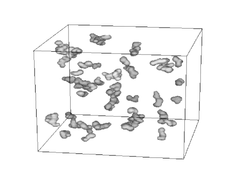
Figure 3: The 3D distribution of our detected superclusters (based on the $\Lambda$CDM₁ cluster sample). A Gaussian smoothing has been applied with 1$\sigma$ radius of 6 $h^{-1}$ Mpc. The elongated prolate-like nature of the detected superclusters is evident.

We have performed a further test in order to verify whether the detected superclusters are the optimal ones. To this end we compare the number of detected $\Lambda$CDM superclusters for different values of the percolation radius with those detected, for the same radius, in random samples of clusters having the same space number density as the simulation clusters. We run a large number of Monte-Carlo simulations in which we destroy the intrinsic $\Lambda$CDM clustering by randomizing the spatial coordinates of the clusters. On this intrinsically random cluster distribution, we apply the procedure described before and identify the random superclusters, $N_{\rm ran}$, which are due to our supercluster-identification method itself.

We define the probability that the detected supercluster in the simulated data is real as ${\cal P}=1-N_{\rm ran}/N_{\rm sup}$. In Fig. 4 we plot that probability depending on the percolation radius for the $\Lambda$CDM₁ (solid line) and $\Lambda$CDM₂ (dashed line) cluster samples. If the percolation radius is significantly smaller than the mean random intercluster separation then the number of random supercluster is null and thus ${\cal P}\simeq 1$. As the percolation radius increases then the number of random superclusters increases as well, but with a slower rate than the corresponding number in a clustered distribution. However, there is a trade-off which has to do with the fact that at extremely small percolation radii, although we ensure that ${\cal P}\simeq 1$, we get a very small number of superclusters. Therefore, the necessity of having adequate statistics leads to a larger percolation radius.

Figure 4: The probability that the supercluster detected in the simulated data with 10 or more members is real as a function of the percolation radius $R_{\rm pr}$. The solid line is for the $\Lambda$CDM₁ sample, the dashed for $\Lambda$CDM₂.

Since in the present study we wish to investigate the morphological characteristics of superclusters and possible related environmental effects, we limit our analysis to superclusters with more than 9 cluster members, for which we can robustly determine their shapes (eg. Kolokotronis et al. 2002). We then find, for the percolation radii determined by eq.(1), ie., $R_{\rm pr}\simeq 18$ and $11\;h^{-1}$ Mpc for the $\Lambda$CDM₁ and the $\Lambda$CDM₂ samples respectively, that the significance (which can be read from Fig. 4) is ${\cal P}>0.95$.

An interesting property of our detected $\Lambda$CDM superclusters is a correlation between the supercluster mass, defined as the sum of the cluster members mass, and the cluster velocity dispersion within their parent superclusters, of the form $M_{\rm sup}\propto\sigma^{\alpha}$ (see Fig. 5). For superclusters with 4 or more members we find that the linear correlation coefficient in log-log space is $\sim 0.4$ with the probability of random correlation being extremely small ($<10^{-7}$) for both $\Lambda$CDM₁ and $\Lambda$CDM₂ cluster samples. The corresponding slopes of the $M-\sigma$ relation is $\sim 0.43\pm 0.08$ and $\sim 0.56\pm 0.06$, respectively. Although the supercluster crossing time along their major axis is much larger than the age of the universe, $t_{u}$, and thus superclusters have not yet turned around (see also Gramann & Suhhonenko 2002), such a correlation imply that they could be “locally” bound (eg. Barmby & Huchra 1998; Small et al. 1998). In fact, many superclusters have crossing times along their minor axis less than $t_{u}$. This is shown in Fig. 6 for the $\Lambda$CDM₁ (left panel) and $\Lambda$CDM₂ (right panel) cluster samples.

Furthermore, it is interesting that supercluster scale peculiar velocities can produce distinct features on the CMB and thus provide the means for detection of superclusters at cosmological distances (eg. Diaferio, Sunyaev & Nusser 2000).

Figure 5: The $M_{\rm sup}-\sigma$ relation for $\Lambda$CDM rich superclusters (with 10 or more members). Left Panel. Based on rich clusters ($\Lambda$CDM₁ sample). Right Panel. Based on poorer clusters ($\Lambda$CDM₂ sample).

Figure 6: The frequency distribution of superclusters with 4 or more members having their crossing times (along their minor axis) indicated along the x-axis. Left Panel. Based on rich clusters ($\Lambda$CDM₁ sample). Right Panel. Based on poorer clusters ($\Lambda$CDM₂ sample).

3.2 Application of the Shapefinder Statistic

To identify the characteristic morphological features of the large scale structures, we will use a differential geometry approach, called “shapefinders” and introduced by Sahni et al. (1998).

The supercluster shapes are defined by fitting ellipsoids to the distribution of cluster members. In Kolokotronis et al. (2002) we investigated the minimum number of points that are necessary in order to determine unambiguously the true shape of a structure traced by a point process. Here we estimate shapes for those superclusters that consist of at least 10 cluster members.

In the case of clusters we can define the shape directly from the distribution of dark matter or gas particles. In both cases we use the moments of inertia method (eg. Carter & Metcalfe 1980; Plionis, Barrow & Frenk 1991). Summing up over the DM or gas particles (for the case of clusters) or the cluster members (for the case of supercluster) we define the inertia tensor:

$$I_{\alpha\beta}=\sum_{i}m^{(i)}x^{(i)}_{\alpha}x^{(i)}_{\beta}.$$ (2)

which after diagonalisation provides the eigenvalues $\alpha_{1}$, $\alpha_{2}$, and $\alpha_{3}$ and the corresponding eigenvectors which point into the direction of the principal axes. Since the eigenvalues can be considered as the three principal axes of the triaxial ellipsoid with the volume $V=\frac{4\pi}{3}\alpha_{1}\alpha_{2}\alpha_{3}$ we can now relate the shape of the configuration to the shape of that ellipsoid.

Below we present the main features of the shape statistic, following the notations of Sahni et al. (1998) (for a first application to astronomical data see Basilakos et al. 2001). To characterize the shape of any object these authors introduced a set of three quantities, defined by ${\cal H}_{1}=VS^{-1}$, ${\cal H}_{2}=SC^{-1}$ and ${\cal H}_{3}=C$, where $V$ is the volume, $S$ the surface and $C$ the integrated mean curvature of the given object. These quantities have dimensions of length and are normalized to give ${\cal H}_{i}=R$ for a sphere of radius $R$. With those quantities one can define two dimensionless shapefinders: $K=(K_{1},K_{2})$, where

$$K_{1}=\frac{{\cal H}_{2}-{\cal H}_{1}}{{\cal H}_{2}+{\cal H}_{1}}$$ (3)

and

$$K_{2}=\frac{{\cal H}_{3}-{\cal H}_{2}}{{\cal H}_{3}+{\cal H}_{2}}\;\;.$$ (4)

The above technique characterizes the shapes of topologically non-trivial cosmic objects according to the following classification:

1. Pancakes if $K_{1}/K_{2}>1$

2. Filaments if $K_{1}/K_{2}<1$

3. Ribbons for $(K_{1},K_{2})\simeq(\alpha,\alpha)$ with $\alpha\leq 1$ and thus structures $K_{1}/K_{2}\simeq 1$ and

4. Spheres if $\alpha_{1}=\alpha_{2}=\alpha_{3}$ and thus $K_{1}=K_{2}=0$

5. ideal filament (one-dimensional objects) for ${\cal H}_{1}\simeq{\cal H}_{2}<<{\cal H}_{3}$

6. ideal pancake (two-dimensional objects) for ${\cal H}_{1}<<{\cal H}_{2}\simeq{\cal H}_{3}$

7. ideal ribbon for ${\cal H}_{1}<<{\cal H}_{2}<<{\cal H}_{3}$

Ideal filaments (0,1), pancakes (1,0), ribbon structures (1,1) and spheres (0,0) are represented by the four vertices of the shape plane in the form of the shape vector $K=(K_{1}$, $K_{2}$), whose amplitude and direction determines the morphology of an arbitrary 3D surface. Finally, for the quasi-spherical objects the $K_{1,2}$ are small and therefore their ratio ($K_{1}/K_{2}$) measures the deviation from perfect spherical shapes. Note that below we will consider as spherical all simulated objects that have $K_{1},K_{2}<0.005$, the axis ratios of which lie in the range: $1\leq\alpha_{1}/\alpha_{3}\leq 1.20$ with $\langle\alpha_{1}/\alpha_{3}\rangle\simeq 1.10\pm 0.06$ and $1\leq\alpha_{1}/\alpha_{2}\leq 1.25$ with $\langle\alpha_{1}/\alpha_{3}\rangle\simeq 1.15\pm 0.05$.

3.2.1 The Shape of DM and Gas Cluster Halos

Using the above procedure we have estimated the shape of both the Dark Matter and the gas component of the $\Lambda$CDM clusters. We have performed this analysis for two minimal spanning tree linking parameters: for the nominal value of 0.17 and for $0.17/2^{n}$ with $n=1$ (probing densities $8^{n}$ times larger than in the former case and hence the inner dense cluster cores). In Fig. 7 we present the corresponding shape spectrum for the $\Lambda$CDM₁ (left panel) and the poorer $\Lambda$CDM₂ cluster samples (right panel). The main panels show the results based on the Dark Matter cluster component while the inner panels to the corresponding gas component. The DM cluster component of both the $\Lambda$CDM₁ and $\Lambda$CDM₂ cluster samples show a strong preference for filamentary-like (prolate-like) configurations with $\sim$ 75% and 72% of the clusters having $K_{1}/K_{2}<1$ while only 1.7% and 2.5% can be considered spherical. Note that in the main panels of Fig.7 the shaded histogram corresponds to the larger linking length while the dashed line to the smaller one. The results based on the Dark Matter cluster component are very similar for both linking parameters indicating that both the inner cluster dark matter core and the cluster outskirts have a consistent shape.

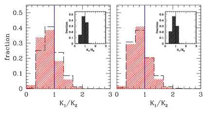
Figure 7: The cluster halo shape spectrum: Left Panel. Rich clusters ($\Lambda$CDM₁ sample), Right Panel. Poorer clusters ($\Lambda$CDM₂ sample). The shaded histograms correspond to a linking parameter of 0.17 ($\rho/\rho_{\rm mean}\simeq 330$) while dashed lines to the denser (by a factor of $\sim 8$) core cluster region (linking parameter of 0.085). The insert shows the corresponding results for the gas cluster component.

Regarding the gas cluster component the results are quite different. As can bee seen from the insert of Fig.7 the shape spectrum peaks at $K_{1}/K_{2}\simeq 1$ with little dispersion around this value. This result together with the quite small values of the $K_{1}$ and $K_{2}$ parameters indicate that the gas distribution is much more spherical than the corresponding dark matter component, as expected. We find that the fraction of clusters having a spherical gas component is 53% and 64% for the $\Lambda$CDM₁ and $\Lambda$CDM₂ cluster samples respectively, while for the smaller linking parameter (the dense cluster cores) the corresponding values are $\sim 44\%$ and $49\%$. This indicates that the gas distribution in the cluster cores is more flattened than in the cluster outskirts. Furthermore, the sphericity of the gas halos implies that the position angles orientations of gas halos are ill-defined and thus should be used in alignment studies with great caution. To visualize this effect we present in Fig. 8 the misalignment angle between the major axes of the DM and gas mass halos as a function of the ratio of the gas halo minor to major axis. Values of the latter near unity imply spherical gas halo shapes. It is evident that indeed the large misalignment angles are correlated with the gas halo sphericity.

Figure 8: Gas halo sphericity versus the misalignment angle between the major axis of the DM and gas cluster halo components for the main linking parameter used (0.17). Left Panel. Rich clusters ($\Lambda$CDM₁ sample), Right Panel. Poorer clusters ($\Lambda$CDM₂ sample).

Finally, in order to test possible resolution effects on the halo shapes, we present in Fig. 9 a comparison of the DM and gas halo axis ratio distribution ($M_{DM}>6\times 10^{13}$ $M_{\odot}$) in the 512³ simulation with the same quantities obtained from another run of the same simulation with 8 times coarser mass resolution ($2\times 256^{3}$ gas and DM particles, see §2.1 for details) It is evident that the DM axis ratio distributions (left panel) are indistinguishable while there is a small effect for the case of the gas halos (right panel), in the direction of having artificially lower gas halo sphericity in the lower resolution simulation.

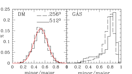
Figure 9: Comparison of the DM and Gas halo sphericity as a function of simulation resolution. In the left panel we also plot, as a continuous line, the Jing & Suto (2002) model which fits well the DM halo axis ratio distribution.

3.2.2 The Shape of Superclusters

In Fig.10 we show the shape spectrum of the detected superclusters (with 10 or more members - dashed-line histograms) and we compare with the corresponding spectrum of their cluster members (for a linking parameter of 0.17). It is obvious that the dominant shape of cosmic structures, being clusters or superclusters, is that of prolate structures (filaments), in agreement with previous theoretical and observational studies (eg. Plionis et al. 1991; Basilakos, Plionis & Maddox 2000; Sathyaprakash et al. 1998; Basilakos et al. 2001; Kolokotronis et al. 2002; Basilakos 2003; Einasto et al. 2003). Furthermore, it is clear that superclusters are more flattened structures than clusters themselves, populating a larger region in the shape-spectrum.

We have verified the dominance of filamentary supercluster shapes for the “optimal” percolation radius, given by eq. (1), although it appears that superclusters have a slightly lower filamentariness with respect to their cluster members. The relevant fractions are: filaments ($\sim 64\%$), pancakes ($\sim 32\%$) and ribbons ($\sim 4\%$). Note that there are no spherical superclusters.

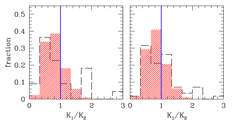
Figure 10: Comparison of the shape spectrum of superclusters containing 10 or more clusters (dashed-line histogram) and of the DM clusters for the two subsamples (left and right figure).

We have further investigated the dependence of the supercluster shape on the value of the percolation radius and we present our results in Fig. 11 where we plot the fraction of superclusters having a filament-like shape ($K_{1}/K_{2}<1$). It is evident that for the richer cluster sample (left panel of Fig. 11), the filamentariness is a dominant feature only around the “optimal” percolation radius (indicated by the arrow). Similarly, for the poorer cluster sample (right panel) the “optimal” percolation radius coincides with a local maxima in the filamentary fraction. However, in this cluster sample, the filamentariness appears to be a generic feature, almost independent of the percolation radius used.

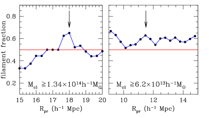
Figure 11: The fraction of filamentary superclusters as a function of percolation radius used to define the superclusters. The arrow indicates the “optimal” percolation radius given by eq.(1). Left Panel. Rich clusters ($\Lambda$CDM₁ sample), Right Panel. Poorer clusters ($\Lambda$CDM₂ sample).

4 The Environmental Trends of the Large Scale Network

4.1 Correlations of vector alignments

As already mentioned in the introduction, an interesting question regarding environmental effects on large scales is whether clusters are aligned with the orientation of their parent supercluster. To study the possible supercluster - clusters alignment we attach to each cosmic structure (being either supercluster or cluster) the orientation as three unit vectors along the three main axes.

Table 2: Correlation analysis results for the different pairs $x,y$ using the cluster DM component. The straight lines in Fig.12 represent the least-square fit to the data and have the general form $y=\lambda x+\beta$. Also, ${\cal R}$ is the correlation coefficient with the corresponding probability (${\cal P}_{R}$) of random correlation. Note that $M_{\rm sup}$ has units of $10^{14}h^{-1}M_{\odot}$.

Sample	Pair $x,y$	$\lambda$	$\beta$	${\cal R}$	${\cal P}_{R}$
$\Lambda$CDM1	$K_{1}/K_{2}$, ${\cal A}(\alpha_{1})$	-0.04$\pm 0.02$	0.63$\pm 0.02$	-0.39	7.9$\times 10^{-2}$
	$K_{1}/K_{2}$, $M_{\rm sup}$	9.3$\pm 4.2$	31.2$\pm 4.4$	0.45	3.8$\times 10^{-2}$
$\Lambda$CDM2	$K_{1}/K_{2}$, ${\cal A}(\alpha_{1})$	-0.05$\pm 0.02$	0.60$\pm 0.02$	-0.29	3.6$\times 10^{-2}$
	$K_{1}/K_{2}$, $M_{\rm sup}$	-	-	-0.11	0.40

The distance vector between the supercluster center of mass and the cluster member is ${\bf r}$, and the normalized direction is ${\hat{\bf r}}={\bf r}/r$. Based on the notations of Beisbart et al. (2002) we consider the following alignment estimator (see also Stoyan & Stoyan 1994; Faltenbacher et al. 2002):

$$A(r)=\langle|{\bf e_{l}}\cdot{\bf e_{k}}|\rangle(r)\;\;.$$ (5)

Therefore, for each supercluster $l$, the factor $A(r)$ describes the direct alignment of the corresponding vector ${\bf e_{l}}$ with the vectors ${\bf e_{k}}$ of the clusters within the parent supercluster. Note that $A(r)$ is proportional to the cosine of the angle between ${\bf e_{l}}$ and ${\bf e_{k}}$. The case of a random alignment signal implies $A(r)=0.5$.

4.2 Shape-Alignment Correlation

In Fig.12 (top panels) we present the alignment $A(\alpha_{1})$ estimator as a function of the supercluster shape, given by the ratio $K_{1}/K_{2}$. There is an obvious supercluster shape-alignment relation, seen in both cluster catalogues ($\Lambda$CDM₁ and $\Lambda$CDM₂), with supercluster alignment increasing with supercluster filamentariness. Furthermore, only for the high cluster mass sample, there is also a significant correlation between the supercluster mass and shape, with mass decreasing with increasing filamentariness. Probably, this is to be expected since pancake-like structures, being two-dimensional should be more massive than the one-dimensional filaments. However this is not observed in the case of $\Lambda$CDM₂.

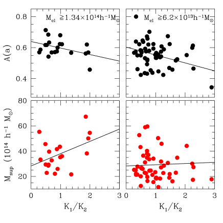
Figure 12: The shape-alignment (upper panels) and shape-mass (lower panels) correlations for the two supercluster samples analyzed and at $a=0.8\alpha_{1}$. The solid lines are the best least-square fits to the data (see Table 2).

Table 2 summarizes the quantitative correlation results for all tests using the cluster DM halo orientations. Probably due to the small number of superclusters (especially in the higher cluster mass sample) the significance of the correlations is not very high. In order to test whether the signal could be affected by a few cluster outliers at the supercluster edges, we have derived the correlation signal and its significance as a function of the parametrized distance of the member clusters from the supercluster center of mass (ie., as a function of $r/\alpha_{1}$, where $r$ is the physical size of the supercluster and $\alpha_{1}$ is its major axis). In Fig.13 we present our results from which it is evident that the signal is relatively stable, although it appears to be higher and more significant around $r/\alpha_{1}\sim 0.8$, indicating that indeed at larger distances, some cluster outliers do reduce the correlation signal.

We have also used the gas halo orientations to repeat the same analysis but as expected from the results presented in section 3.2.1 (see Fig. 8) we do not find a significant signal for the $\Lambda$CDM₁ sample. However, for the poorer $\Lambda$CDM₂ sample we have found a correlation signal (${\cal R}=-0.25$) with a random probability of ${\cal P}\simeq 0.07$.

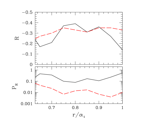
Figure 13: The shape-alignment correlation coefficient (upper panel) and random probability (lower panel) as a function of supercluster-centric distance.

Furthermore, we have seen in Fig. 11 that the fraction of filamentary superclusters depend on the percolation radius used and thus if, as suggested by the correlations in Table 2 and Fig. 12, the alignment signal is higher in the filamentary superclusters we may expect a drop of the signal when the distribution of superclusters is dominated by pancake-like morphologies. Therefore, in order to investigate the above as well as the robustness of the correlation signal we re-assigned cluster DM halos to superclusters using a range of percolation radii, around the “optimal” value given by eq.(1). In Fig. 14 we present both the value of the shape-alignment correlation coefficient and its random probability as a function of percolation radius used to define the superclusters. The resulting correlation coefficients is higher and more significant very near the “optimal” percolation radius, defined by eq.(1), which also coincides with peaks in the distribution of supercluster filamentary fraction (Fig.11).

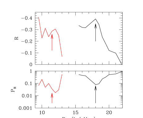
Figure 14: The shape-alignment correlation coefficient (upper panel) and random probability (lower panel) as a function of percolation radius used to define the superclusters. The arrow indicates the values corresponding to the “optimal” percolation radius. The graphs on the right and left correspond to the lower ($\Lambda$CDM₂) and higher ($\Lambda$CDM₁) mass samples.

The increase of the supercluster filamentariness with alignment, is to be expected according to the hierarchical clustering scenario, where gas and galaxies flow into denser regions along anisotropic directions, defined by the large-scale structure (cf. West 1994; Ostriker & Cen 1996 and references therein). As a result of these inflows we expect clusters to be aligned with their neighbours, especially when both are members of the same filament. For low-$\Omega_{\rm m}$ cosmologies one expects that major merging and anisotropic accretion of matter along filaments will have stopped long ago. Thus gravitational violent relaxation would tend to isotropize the cluster phase-space configuration, more so in the recent times. However, it has been shown that clusters retain memory of their initial anisotropic configuration from were they accreted the main bulk of the matter that they contain (eg. van Haarlem & van de Weygaert 1993).

4.3 Supercluster - cluster velocity correlations

In this section we investigate possible correlations between the supercluster shapes and the alignment between supercluster major axis and their member cluster velocity field. Using the notations of section 4.1 we can define the following cross-correlation vector estimator:

$$U(r)=\langle|{\bf e_{l}}\cdot{\bf v_{k}}|\rangle(r)$$ (6)

where $\bf v_{k}$ is velocity vector with $|{\bf v_{k}}|=1$, which corresponds to each host cluster while ${\bf e_{l}}$ is the eigenvector of the major ($r=\alpha_{1}$) supercluster axis.

We find that shape - velocity alignment correlations does not exist at any significant level. However, for the case of high mass clusters ($\Lambda$CDM₁ sample) there is a relatively significant correlation between $A(r)$ and $U(r)$, indicating that the alignment between supercluster and cluster member major axes is accompanied with a similar alignment between supercluster major axis and the direction of the cluster member peculiar velocity (see Fig. 15).

Figure 15: The cluster velocity -supercluster alignment $[U(r)]$ and cluster major axis-supercluster alignment $[A(r)]$ correlation for the $\Lambda$CDM₁ superclusters.

5 Conclusions

We have studied the morphological features of $\Lambda$CDM cluster dark matter and baryonic gas halos as well as superclusters using a large volume ($V=500^{3}\;h^{-3}$ Mpc³) N-body+GADGET simulation with unprecedented mass resolution. The measure of the structure geometry has shown that prolate-like (filamentary) shapes dominates over pancakes, in agreement with other recent large-scale structure studies. We have also presented evidence that there is a specific link between the orientation of cluster dark matter halos and that of the large scale network. Cluster size halos appear to be aligned with their parent supercluster major axis, more so if the supercluster is filamentary-like. For the richest cluster halos we have also found a correlation between the halo peculiar velocity - supercluster alignment and the cluster major axis-supercluster alignment signals.

References

- [] Bahcall N., Ann. Rev. Astr. Ap., 1988, 26, 631
- [] Bahcall N., Soneira R., 1984, ApJ, 277, 27
- [] Bahcall, N., &, Burgett, W. S., 1986, ApJ, 300, L35
- [] Bahcall, N., &, West, M. J., 1992, ApJ, 392, 419
- [] Basilakos, S., Plionis, M., Maddox, S.J., 2000, MNRAS, 316, 779
- [] Basilakos S., Plionis M., Rowan-Robinson M., 2001, MNRAS, 223, 47
- [] Basilakos S., 2003, MNRAS, 344, 602
- [] Basilakos, S., Plionis, M., 2004, MNRAS, 349, 882
- [] Bailin J., &, Steinmetz M., 2005, ApJ, 627, 647
- [] Barmby, P., Huchra, J.P., 1998, AJ, 115, 6
- [] Beisbart, C., Kerscher, M., Mecke, K., &, Matthias, 2002, Lecture Notes in Physics, second Wuppertal conference ”Spatial statistics and statistical physics”, physics/0201069
- [] Bhavsar, S.P., & Splinter, R.J. 1996, MNRAS 282, 1461
- [] Binggeli B., 1982, A&A, 107, 338
- [] Böhringer, H., et al., 2001, A&A, 369, 826
- [] Carter, D., &, Metcalfe, N., 1980, MNRAS, 191, 325
- [] Chambers S. W., Melott A., Miller C., 2002, ApJ, 565, 849
- [] Colberg, J. M, et al., 2000, MNRAS, 319, 209
- [] Collins, C. A., et al., 2000, MNRAS, 319, 939
- [] Dalton, B. G., Croft, R. A. C., Efstathiou, G., Sutherland, W. J., Maddox, S. J., Davis, M., 1994, MNRAS, 271, L47
- [] de Lapparent V., Geller M. J., Huchra J. P., 1991, ApJ, 369, 273
- [] Diaferio, A., Sunyaev, R.A., Nusser, A, 2000 ApJ, 533, L71
- [] Diaferio, A., Nusser, A., Yoshida, N., Sunyaev, R.A., 2003, MNRAS, 338, 433
- [] Dubinski, J., 1994, ApJ, 431, 617
- [] Efstathiou, G., Bernstein, G., Tyson, J.A., Katz, N., Guhathakurta, P., 1991, ApJ, 380, L47
- [] Einasto M., Tago E., Einasto J., Andernach H., 1997, A&AS, 123, 119
- [] Einasto M., Einasto J., Tago E., Mueller V., Andernach H., 2001, AJ, 122, 2222
- [] Einasto J., et al., 2003, A&A, 410, 425
- [] Einasto M., Suhhonenko, I., Heinamaki, P., Einasto J., Saar, E., 2005, A&A, 436, 17
- [] Faltenbacher, A., Gottlöber, S., Kerscher, M.; Müller, V., 2002, A&A, 395, 1
- [] Frenk, C. S., White, S. D. M., Davis, M., Efstathiou, G., 1988, ApJ, 327, 507
- [] Faltenbacher, A., Allgood, B., Gottlöber, S., Yepes, G., Hoffman, Y., 2005, MNRAS, 362, 1099
- [] Flin, P., 1987, MNRAS, 228, 941
- [] Frisch S.F. P. et al., 1995, A&A, 296, 611
- [] Goto, T., et al., 2002, AJ, 123, 1807
- [] Gramann, M. & Suhhonenko, I., 2002, MNRAS, 337, 1417
- [] Hopkins, P. F., Bahcall, N. A., Bode, P., 2005, ApJ, 618, 1
- [] Ikebe, Y., Reiprich, T.H., Böhringer, H., Tanaka, Y., & Kitayama, T. 2002, A&A, 383, 773
- [] Jing, Y.P., &, Suto, Y., 2002, ApJ, 574, 538
- [] Kasun S.F., &, , Evrard, A.E., 2005, ApJ, 629, 781
- [] Klypin, A.,Gottlöber, S., Kravtsov, A.V., Khokhlov, A.M., 1999, ApJ, 516, 530
- [] Kolokotronis, V., Basilakos, S., Plionis, 2002, MNRAS, 331, 1020,
- [] Lee, J., Kang, X., Jing, Y., 2005, ApJ, 629, L5
- [] Onuora, L. I., &, Thomas, P. A., 2000, MNRAS, 319, 614
- [] Oort, J.H., 1983, ARA&A, 21, 373
- [] Ostriker, J. P., &, Cen, R., 1996, ApJ, 464, 27O
- [] Pandey, B., &, Bharadwaj, S., 2005, MNRAS, 357, 1068
- [] Peebles P. J. E., 2001, ApJ, 557, 495
- [] Pimbblet, K. A., 2005, MNRAS, 358, 256
- [] Plionis M., Barrow J.D., Frenk C.S., 1991, MNRAS, 249, 662
- [] Plionis M., Valdarnini, R., Jing, Y.P., 1992, ApJ, 398, 12
- [] Plionis, M., 1994, ApJS, 95, 401
- [] Plionis, M., & Basilakos, S., 2002, MNRAS, 329, L47
- [] Plionis, M., Benoist, C., Maurogordato, S., Ferrari, C., Basilakos, S., 2003, ApJ, 594, 144, 2003
- [] Plionis, M.,2002, in Modern Theoretical and Observational Cosmology, Proceedings of the 2nd Hellenic Cosmology Meeting, Astrophysics and Space Science Library, Vol. 276, Kluwer Academic Publishers, Dordrecht, 2002., p.299
- [] Plionis, M., 2004, Outskirts of Galaxy Clusters: Intense Life in the Suburbs, Proceedings of IAU Symposium, No. 222., Cambridge University Press, 2004., p.19-25
- [] Rhee, G., &, Katgert, P., 1987, A&A, 183, 217
- [] Sahni V., Sathyaprakash B. S., Shandarin S., 1998, ApJ, 495, L5
- [] Sathyaprakash S. B., Sahni V., Shandarin S., 1998, ApJ, 508, 551
- [] Shandarin, S.F., Sheth, J.V., Sahni, V., 2004, MNRAS, 353, 162
- [] Sheth, R. K., & Tormen, G. 1999, MNRAS, 308, 119
- [] Sheth, J. V., Sahni, V., Shandarin, S. F., Sathyaprakash, B.S., 2003, MNRAS, 343, 22
- [] Springel V., Yoshida N., White S. D. M., 2001, New Astronomy, 6, 79
- [] Springel V., &, Hernquist, L., 2002, MNRAS, 333, 649
- [] Struble, M. F., &, Peebles, P. J. E., 1985, AJ, 90, 582
- [] Stoyan D. &, Stoyan, H., 1994, Fractals Randon Shapes and Point Fields (Chichester: John Wiley & Sons)
- [] Small, T.A., Ma, C.P.; Sargent, W.L.W.; Hamilton, D., 1998, ApJ, 492, 45
- [] Ulmer, M., McMillan, S. L. W., Kowalski, M. P., 1989, 338, 711
- [] van Haarlem, M.P., van de Weygaert, R., 1993, ApJ, 418, 544
- [] van Haarlem, M. P., Frenk, C. S., White, S. D. M., 1997, MNRAS, 287, 817
- [] West J. M., 1989, ApJ, 347, 610
- [] West J. M., 1994, MNRAS, 2668, 79
- [] West J. M., Jones, C., Forman, W., 1995, ApJ, 451, L5
- [] Yepes, G., Ascasibar, Y., Sevilla, R., Gottlöber, S. & Müller, V., 2004, Proceedings of IAU Colloquium 195 “Outskirts of Galaxy Clusters: Intense Life in the suburbs”, Ed. A. Diaferio, Cambridge Univ. press, pag. 274.
- [] Zeldovich, Ya. B., Einasto, J., Shandarin, S., 1982, Nature, 300, 407