The Core-Collapse Supernova
with “Non-Uniform” Magnetic Fields

Abstract

We perform two-dimensional numerical simulations on the core-collapse of a massive star with strong magnetic fields and differential rotations using a numerical code ZEUS-2D. Changing field configurations and laws of differential rotation parametrically, we compute 14 models and investigate effects of these parameters on the dynamics. In our models, we do not solve the neutrino transport and instead employ a phenomenological parametric EOS that takes into account the neutrino emissions. As a result of the calculations, we find that the field configuration plays a significant role in the dynamics of the core if the initial magnetic field is large enough. Models with initially concentrated fields produce more energetic explosions and more prolate shock waves than the uniform field. Quadrapole-like fields produce remarkably collimated and fast jet, which might be important for gamma-ray bursts(GRB). The Lorentz forces exerted in the region where the plasma-beta is less than unity are responsible for these dynamics. The pure toroidal field, on the other hand, does not lead to any explosion or matter ejection. This suggests the presupernova models of Heger et al. (2003), in which toroidal fields are predominant, is disadvantageous for the magnetorotation-induced supernova considered here. Models with initially weak magnetic fields do not lead to explosion or matter ejection, either. In these models magnetic fields play no role as they do not grow on the timescale considered in this paper so that the magnetic pressure could be comparable to the matter pressure. This is because the exponential field growth as expected in MRI is not seen in our models. The magnetic field is amplified mainly by field-compression and field-wrapping in our simulations.

1 Introduction

The study of magnetorotational core-collapse supernovae is currently attracting great attention. This is mainly because anomalous X-ray pulsars (AXP) (Thompson & Duncan, 1996) and soft gamma-ray repeaters (SGR) (Duncan & Thompson, 1992) have been discovered and thought to be candidates of magnetar. The magnetar is a sub-class of pulsar which has an extraordinarily large magnetic field, $\sim$ $10^{14}$ - $10^{15}$ gauss. This value is two to three orders of magnitude greater than that of the ordinal pulsar. So far, only about ten of them have been observed and little is known of them. The formation mechanism, in particular, is veiled in mystery.

Ordinary pulsars are thought to be formed as a result of core-collapse supernovae, and so are magnetars. Then, it is necessary to study magnetorotational core-collapse supernovae. Since the number of magnetars is smaller than that of ordinary pulsars by a factor of $\sim 100$, they form a particular group and there may be a special condition for a progenitor, such as large magnetic field or rapid rotation, for their formation. The main purpose in this paper is to systematically study the dynamics of core-collapse with very strong magnetic fields and rapid rotations. It may be possible that the study of this extraordinary supernovae have some implication also for the ordinary supernovae mechanism which produces normal pulsars.

The mechanism of ordinary supernovae is still unknown. The recent spherically symmetric simulations which employ a realistic equation of state (EOS) and sophisticated microphysics such as the neutrino transport and/or the electron capture (Rampp & Janka, 2000; Liebendörfer et al., 2001; Thompson et al., 2003; Buras et al., 2003; Liebendörfer et al., 2004; Sumiyoshi et al., 2004) have not found successful explosions. On the other hand, core-collapse supernovae might be generically asymmetric (Wang et al., 1996; Leonard et al., 2000). SN1987A is a clear example, which is indicated by the HST image of the asymmetrically expanding envelope (Wheeler et al., 2000, and references therein). Rotation of progenitors is a natural choice for the cause of asymmetry although the instability of the standing accretion shock may be another candidate (Foglizzo & Tagger, 2000; Blondin et al., 2003). Some authors claimed that rotation and asymmetric neutrino radiation induced thereby may be crucially important for the explosion (Shimizu et al., 2001; Kotake et al., 2003; Yamasaki & Yamada, 2005, but see also Walder et al. (2005) and Janka et al. (2005) for critieisms). On the other hand magnetic fields in massive stars might yet another candidate for the cause of not only asymmetry but also explosion itself. In fact, some researchers are attempting to explain the mechanism for all supernovae with magnetic field (Wheeler et al., 2002).

The first numerical simulation of supernovae with magnetic field and rotation was done about thirty years ago by LeBlanc & Wilson (1970). Some more numerical studies followed them after (e.g. Bisnovatyi-Kogan et al., 1975; Müller & Hillebrandt, 1979; Ohnishi, 1983; Symbalisty, 1984). Although these studies, especially Symbalisty (1984), are important, they had not attracted much attention mainly because there were no observational support that magnetic fields may play an important role in supernovae one way or another. In fact, the field strength inferred from the ordinary pulsar is negligible for the dynamics of core-collapse. The situation, however, may have changed with the discovery of magnetars. The progress of our understanding of the mechanism for field amplification (Balbus & Hawley, 1991) is yet another boost. In the last couple of years, we have seen the study of magnetized supernovae have gained momentum again (e.g. Ardeljan et al., 2000; Wheeler et al., 2002; Akiyama et al., 2003; Yamada & Sawai, 2004; Kotake et al., 2004; Takiwaki et al., 2004; Ardeljan et al., 2004).

The number of numerical models, however, is still not very large. Even the systematics of dynamics for magneto-rotational core-collapse has not been investigated throughly. We studied effects of strong uniform, poloidal magnetic field with rapid rotation systematically, varying the initial field strengths as parameters (Yamada & Sawai, 2004). It was found that the jet-like explosion is produced by the combination of initial large magnetic field and rapid rotation and that the driving force is the amplified magnetic fields in the region between the shock wave and the inner core. In this paper, only the uniform field was considered as an initial field configuration. In fact, the effect of the initial field configuration has not been studied systematically so far. It is true that the initially uniform field does not have a firm basis. As a matter of fact, recent studies of stellar evolution (Heger et al., 2003) suggest that the toroidal fields are dominant prior to the collapse. This is, however, still highly uncertain. Hence, in this paper we investigate how dynamics and field amplifications depend on the initial field configurations, assuming them rather arbitrarily. As mentioned later again in §2.5, we mainly explore a very strong field regime, in which we assume $B\sim 10^{12}-10^{13}$ G initially. However, we also study weak field models with $B\sim 10^{8}-10^{9}$ G for comparison. Our standing point is that we are concerned with the strongly magnetized progenitors, which will produce magnetars and we do not address the origin of such strong magnetic fields for the moment. Since the main purpose is to study the systematics of dynamics, we simplify microphysics and study the phenomena occurring only on the prompt-explosion timescale as in Yamada & Sawai (2004). The present paper is a sequel of Yamada & Sawai (2004).

The paper is organized as follows. We introduce our methods of calculation and models in the next section. The results are presented in §3. In the last section we discuss our results and conclude this paper.

2 Numerical Methods and Models

2.1 Numerical Code

We have carried out two-dimensional axisymmetric magnetohydrodynamic (MHD) simulations with the numerical code ZEUS-2D developed by Stone & Norman (1992). We describe some properties of the code briefly. There are two main difficulties in solving the MHD equations compared to the hydrodynamic (HD) equations. The first one is to deal with the constraint of the magnetic field, and the second one is concerned with the accurate treatment of Alfvén waves. For the first difficulty, ZEUS-2D employs the constrained transport (CT) method instead of solving the vector potential, which would produce false accelerations and heating near shocks or contact surfaces. As for the second problem, the method of characteristics (MOC) is employed in order to avoid incorrect Alfvén modes. In solving the Poisson equation for the gravitational potential, this code utilizes the Incomplete Cholesky decomposition Conjugate Gradient (ICCG) method. Readers are referred to their original paper (Stone & Norman, 1992) for more detail.

2.2 Basic Equations

We solve the ideal MHD equations,

$$\frac{D\rho}{Dt}+\rho\nabla\cdot\mbox{\boldmath$v$}=0,$$ (1)

$$\rho\frac{D\mbox{\boldmath$v$}}{Dt}=-\nabla p-\rho\nabla\Phi+\frac{1}{4\pi}(\nabla\times\mbox{\boldmath$B$})\times\mbox{\boldmath$B$},$$ (2)

$$\rho\frac{D}{Dt}(\frac{e}{\rho})=-p\nabla\cdot\mbox{\boldmath$v$},$$ (3)

$$\frac{\partial\mbox{\boldmath$B$}}{\partial t}=\nabla\times(\mbox{\boldmath$v$}\times\mbox{\boldmath$B$}),$$ (4)

where $\rho$, $v$, $p$, $e$, $\Phi$, $B$ are the density, velocity, internal energy density, gravitational potential, and magnetic flux density, respectively. The Lagrangian derivative is denoted as $\frac{D}{Dt}$.

Assuming the equatorial symmetry, we use the spherical coordinates and solve only the quarter of the meridional plane. Until the central density reaches $10^{12}$ g/cm³, we use 200 ($r$)$\times$ 30 ($\theta$) grid points, extending to 2000 km in the radial direction. Thereafter, the number of grid points and the radius of outer boundary are set to be 300 ($r$)$\times$ 30 ($\theta$) and 1500 km, respectively. In the radial direction, the mesh is non-uniform with finer grids toward the center while the angular grid points are uniform.

2.3 Equation of State

As in the previous paper of Yamada & Sawai (2004), we adopt a parametric EOS which was first introduced by Takahara & Sato (1984). Since our purpose is to investigate effects of the magnetic field configuration on the prompt-explosion timescale and we are mainly concerned with the systematic change of dynamics, we drastically simplify complicated microphysics such as the neutrino transport.

The parametric EOS we employed in this paper is described as follows;

$$p_{tot}=p_{c}(\rho)+p_{t}(\rho,e_{t}),$$ (5)

$$p_{c}(\rho)=K\rho^{\Gamma},$$ (6)

$$p_{t}(\rho,e_{t})=(\gamma_{t}-1)\rho\epsilon_{t}.$$ (7)

The pressure consists of two parts, the cold part ($p_{c}$) and the thermal part ($p_{t}$). The thermal part is a function of the density and the specific thermal energy, $\epsilon_{t}$, in which $\gamma_{t}$ is the parameter called the thermal stiffness. The thermal energy generated by shock dissipation loses its considerable part due to the photodisintegration of neuclei as well as to thermal neutrino emissions. This effect is mimicked in the thermal part of EOS with an appropriate value of the thermal stiffness. On the other hand, the cold part is a function of the density alone where the constants $K$ and $\Gamma$ reflect the effect of the degeneracy of leptons and the nuclear force. The values of $\Gamma$ are given as follows;

$$\Gamma_{1}=\frac{4}{3}\hskip 28.45274pt\textrm{dencity regime \hskip 8.5359pt I}$$ (8)

$$\Gamma_{2}=\frac{\log p_{2}-\log p_{1}}{\log\rho_{2}-\log\rho_{1}}=\frac{4}{3}+\frac{\log d}{\log(\rho_{2}/\rho_{1})}\hskip 98.16191pt\textrm{II}$$ (9)

$$\Gamma_{3}=\frac{4}{3}\hskip 98.16191pt\textrm{III}$$ (10)

$$\Gamma_{4}=2.5\hskip 98.16191pt\textrm{IV}$$ (11)

$$d\equiv\frac{p_{2}}{p_{1}}\sim\Biggl{[}\frac{Y_{l}(\rho_{2})}{Y_{l}(\rho_{1})}\Biggr{]}^{4/3}\hskip 99.58464pt$$ (12)

where $Y_{l}$ is the number of leptons per baryon. The boundary between the regimes I and II corresponds to the onset of the electron capture at density of $\rho_{1}=4.0\times 10^{9}$cm/g³, from which point the adiabatic index decreases. The density $\rho_{2}=1.0\times 10^{12}$ g/cm³, the boundary of the regimes II and III, is the point at which the neutrino trapping is commenced. Then the electron capture ceases and the adiabatic index increases again. After the density reaches $\rho_{3}=2.8\times 10^{14}$ g/cm³, the pressure becomes nuclear-force-dominant and adiabatic index rises considerably. In this EOS, we can specify two parameters, the thermal stiffness $\gamma_{t}$ and the lepton fraction $d$. According to the papers by Takahara & Sato (1984) and Yamada & Sato (1994) which also used this EOS, larger $\gamma_{t}$ and $d$ are favorable for successful prompt explosions. Here we adopt 1.3 for thermal stiffness and 0.78 for lepton fraction by setting $Y_{l}(\rho_{2})=0.35$ which corresponds to 1.29 for the adiabatic index in the density regime II. Note that recent sophisticated spherically symmetric simulations suggest that the lepton fraction at the onset of neutrino trapping is $\sim 0.35$ (e.g. Liebendörfer et al., 2004). With these parameters, our spherically symmetric model does not lead to a successful explosion as in recent realistic simulations.

2.4 Progenitor

We use the central $1.4M_{\odot}$ core of the $15M_{\odot}$ presupernova stellar model by Woosley (1995), which provides us with the spherically symmetric profile of the density and the specific internal energy. We add by hand magnetic field and rotation to the original model, which will be explained in detail in §2.5.

2.5 Magnetic field and Rotation

The most important ingredients in this study are magnetic field and rotation. Changing these parameters, we have computed 14 models. We adopt four different types of field configurations as follows. The first one, which is the simplest and has been employed in most of the past simulations, is uniform field parallel to the rotation axis. The second configuration is the one which is parallel to the rotation axis but axially concentrated, and is described as

$$B_{z}=B_{z0}\frac{\varpi_{0}^{2}}{\varpi_{0}^{2}+\varpi^{2}}$$ (13)

where z and $\varpi$ are the cylindrical coordinates, and $B_{z0}$ and $\varpi_{0}$ are constants. One can obtain strong concentration of the field near the axis with small $\varpi_{0}$. The third is quadrapole-like configuration, which was introduced by Ardeljan et al. (1998):

$$B_{\varpi 0}=F_{\varpi}(0.5\varpi,0.5z-2.5)-F_{\varpi}(0.5\varpi,0.5z+2.5),B_{\phi 0}=0,$$

$$B_{z0}=F_{z}(0.5\varpi,0.5z-2.5)-F_{z}(0.5\varpi,0.5z+2.5),$$ (14)

$$F_{\varpi}(\varpi,z)=k\Biggl{(}\frac{2\varpi z}{(z^{2}+1)^{3}}-\frac{2\varpi^{3}z}{(z^{2}+1)^{5}}\Biggr{)},F_{z}(\varpi,z)=k\Biggl{(}\frac{1}{(z^{2}+1)^{2}}-\frac{\varpi^{2}}{(z^{2}+1)^{4}}\Biggr{)},$$

where $k$ is the parameter specifying the strength of magnetic field, and $z$ and $\varpi$ are normalized by $1.6\times 10^{8}$cm. The last type is a pure toroidal configuration which is concentrated with the same law as differential rotation (see below in the text), that is,

$$B_{\phi}=B_{\phi 0}\frac{r_{0}^{2}}{r_{0}^{2}+r^{2}},$$ (15)

where $r$ is the distance from the center, and $B_{\phi 0}$ and $r_{0}$ are constants.

We adopt shell-type differential rotation with the angular velocity distribution,

$$\Omega(r)=\Omega_{0}\frac{R_{0}^{2}}{R_{0}^{2}+R^{2}},$$ (16)

where $\Omega_{0}$ and $R_{0}$ are constants. With small $R_{0}$ strong differential rotation is obtained.

In Table 1, we present 14 models. The name of each model consists of two parts, alphabets and a number. The capital alphabet denote the magnetic field configuration with H, C, Q, T representing the homogeneous, concentrated, quadrapole-like, and toroidal fields, respectively. And the attached number stands for a strength of the field concentration and/or differential rotation. The last three models have a small alphabet (w) implying that its initial magnetic field is very weak. The energy of magnetic field and rotation is set to be 0.5% of the gravitational energy for all models except for the last three ones with w in the name.

According to the recent study on the stellar evolution, a presupernova core may be toroidal-field-dominant and may have a slow rotation velocity (Heger et al., 2003), but there still exist some uncertainty in their models, and the distributions of magnetic field and angular velocity are not well established yet. Observations are not helpful either. Hence our stand point is that we regard these distributions as unknown factors and vary them arbitrarily. If anything, however, model T5w is rather close to that of Heger et al. (2003) at least in the field configuration and strength though the angular velocity is larger.

3 Results

In this section we describe the numerical results of the computation. We mainly focus on the differences in dynamics and field-amplification among the models. In table 2, we show important parameters for all models.

3.1 Dynamics

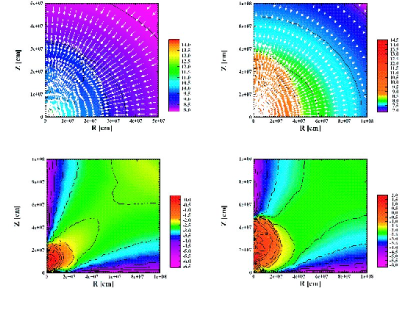
Figure 1: The velocity fields on top of the density color contours for model H10 (top panels), and the contours of the ratio of $p_{mag}/p_{matter}$, where $p_{mag}$ and $p_{matter}$ are magnetic and matter pressures, respectively (bottom two panels). The left figures are drawn for at 14 ms after bounce (152 ms from the beggining) and the right figures for 24 ms after bounce (162 ms from the begining).

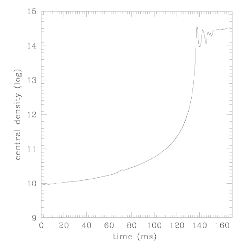
Figure 2: The time evolution of the central density for model H10.

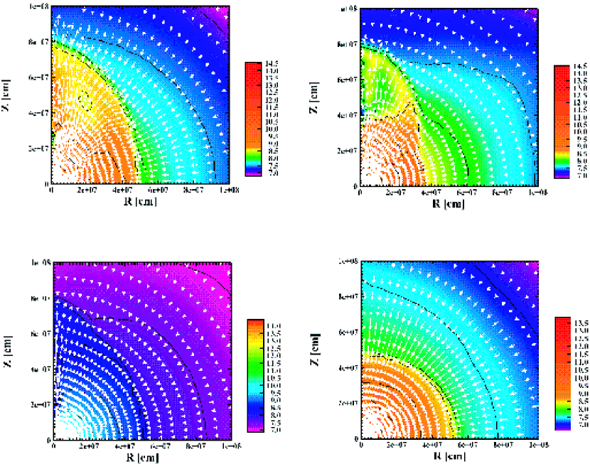
Figure 3: The velocity fields on top of the density contours for model H10 (top left panel), C5 (top right panel), Q10 (bottom left panel) and T5 (bottom right panel). Each panel is depicted for 31 ms, 27 ms, 42 ms and 49 ms after bounce (169 ms, 171 ms, 180 ms and 191 ms from the beggining), respectively.

We chose model H10 as the reference cases and first describe its dynamical evolution for the comparison with other models. The collapsing matter is halted and bounces at 137 ms after the beginning of simulation, when the central density reaches its maximum value, $3.5\times 10^{14}$ g/cm³, and a shock wave is produced. During this collapsing phase, the compression and wrapping of frozen-in magnetic fields generates a strong toroidal field, $\sim 10^{16}$ G. A region where the toroidal magnetic pressure dominates over the matter pressure begins to be formed behind the shock wave a few milliseconds after bounce and prevails along the rotation axis as the shock propagates in a prolate fashion (see Fig. 1). As seen in Fig. 2, the core is oscillating for sometime after bounce, and what we call “small bounces” produce some more shock waves. Since these trains of newborn shocks are further powered by the dominant toroidal magnetic pressure, they gain larger amplitude in the direction of the rotation axis than the first shock wave which is not affected by magnetic pressure strongly and does not have enough energy to penetrate through the core. The first shock is soon catched up with by these large-amplitude waves and acquires sufficient energy to break through the core. Consequently, a strong magnetocentrifugal jet is induced along the rotation axis (see Fig. 3), and it will eventually lead to an axisymmetric bipolar supernova explosion.

On the contrary, no explosion occurs in the pure rotation case (model R10). The bounce occurs at 142 ms with the central density, $2.0\times 10^{14}$ g/cm³. Small bounces occurs also in this model. Lacking in the support by magnetic fields, however, the shocks launched by the small bounces have too small energy to supply energy to the first shock when they catch up with it. Note that the synergically symmetric model does not give an explosion with the current set of the parameters of our EOS.

For the models with initially axially-concentrated magnetic fields, the dynamics is a little different from that of reference model with the uniform field. For model C5, in particular, the first shock is powered not by the nuclear force but by the magnetic force. Slightly prior to the nuclear-force-induced bounce, the magnetic-force-dominant region has already been formed at the boundary of the inner and outer cores. Then the first shock wave is generated and starts to propagate outward. However, it slows down as it goes out of the region where the magnetic pressure is dominant. The second shock generated by nuclear force runs after the first shock and is powered in the magnetic-pressure-dominant region. Subsequent shock waves generated by “small bounce” also gain large energy in the same way. The first shock soon collects energy from these shock waves as in the reference model. At the end of the simulation, a strong axial jet is formed with velocities higher than in model H10. While the jet-collimation is not very different from that of model H10, the shape of shock surface is more prolate with an aspect ratio of 2.0 (see Fig. 3).

For model C10, no shock wave is generated prior to the nuclear-force-induced bounce as in model C5. The shock wave generated by the bounce, however, acquires large energy from subsequent shock waves as in the case of uniform field. The resulting dynamical feature is almost the same as in model C10 though the jet collimation is slightly weaker than that of model H10 or C5 (see Fig. 3).

As shown in Table 2, the stronger the field concentration and differential rotation become, the more prolate the shock is generated and the faster the jet becomes. According to Yamada & Sato (1994), strong differential rotation tends to enhance asymmetry of shock. The comparison of models H10 and C10, which have different concentration of magnetic fields, suggest that the field concentration also tends to make a shock more prolate. The reason is that strong poloidal fields prevent matter from traveling in the transverse direction.

The models with the quadrapole-like configuration have distinct feature, that is, a fast jet and its remarkable collimation with a very small opening angle (see Table 2 and Fig. 3), while the shock surfaces are less prolate than in the uniform or axially-concentrated field cases. In these models both the first shock and subsequent shocks are accelerated toward the rotation axis by the dominant toroidal magnetic pressure. In model Q10, the fastest jet among all models is produced. In this model, the acceleration is very strong especially for a subsequent shock, which is born at 100 km from the center a few ten milliseconds after bounce when the first shock reaches around 500 km. Then this shock soon gains large energy from magnetic pressure, and the matter velocity becomes considerably high, $c/3-c/2$, at the shock front, where $c$ is the light velocity. This large amplitude shock overtakes the first shock and causes the remarkable collimation. We evaluate the parameters in Table 2 when the shock reaches 800 km from the center on the rotation axis. The large-amplitude subsequent shock has not caught up with the first shock yet in model Q10. Although the collimation parameter for Q10 is not small compared with models Q3 or Q5, it will become smaller and comparable to model Q3 later.

In the pure toroidal field cases, we cannot find any substantial deviation from the rotation-only case though they have large magnetic energy. Fig. 3 shows for model T5 that the shock wave stalls around 400 km, and neither explosion nor matter ejection occurs. Moreover, no region appears where the magnetic pressure is dominant through the simulation. This is because the field-wrapping by differential rotation does not occur. It is true that the compression of frozen-in fields during the collapse amplifies the toroidal fields significantly but the field grows as $B\propto\rho^{3/4}$ which is the same as the increase of matter pressure. Hence the ratio of magnetic pressure to matter pressure is unchanged. Note that Kotake et al. (2004) found magnetic-field-dominant regions are formed in their pure toroidal models, which may be ascribed the difference in employed EOS and including microphysics.

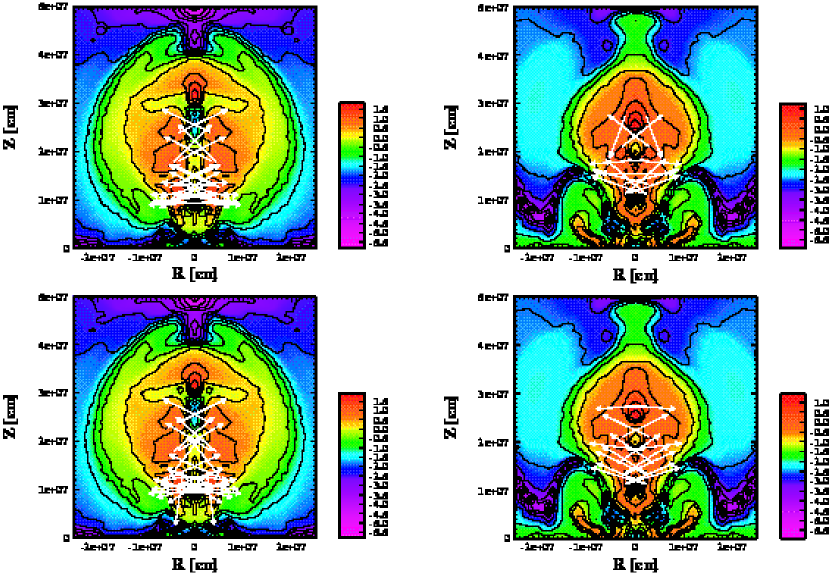
Figure 4: The Lorentz forces (arrows) on top of the color contour of the ratio $p_{mag}/p_{matter}$ for model H10 at 23 ms after bounce (161 ms from the onset of collapse) and for model Q10 at 30 ms after bounce (161 ms from the onset of collapse) (top left and top right panels, respectively). The sum of the Lorentz force and matter-pressure-gradient on top of the same color contour for models H10 and Q10 (bottom left and bottom right panels, respectively) at the same evaluation times as for top figures. The shock is located at about 500 km from the center on the rotation axis. The arrows are drawn only where $p_{mag}$ is greater than $8p_{mattar}$ in the left panels and $\frac{1}{2}p_{mattar}$ in the right panels .

Next, we discuss what causes the differences in dynamics among these models such as the asymmetry of shock front and the jet collimation. We pay attention to the Lorentz force which is the third term in r.h.s of Eq. (2), $\frac{1}{4\pi}(\nabla\times\mbox{\boldmath$B$})\times\mbox{\boldmath$B$}$. In the top panels of Fig. 4 we show the Lorentz force for models H10 and Q10. The lower panels in the figure show the total force field including the matter-pressure-gradient. It can been seen clearly in each case that the Lorentz force thrusts matter to the narrow region around the rotation axis. Even after the pressure gradient which tends to expand matter is added, the total force still squeezes matter and helps to push it more powerfully along the axis.

One can also see the difference between the models; the difference in the width of the magnetic-force-dominant region. This region is wider for model H10 and more matter is forced to collimate to form a jet. For model Q10, on the other hand, the region is narrower and less matter is affected by the Lorentz force, which leads to the remarkable collimation as seen in Fig. 3. The asymmetry of the shock front also depends on the width of the magnetic-field-dominant region. In the models with the initially axially-concentrated fields, this region is narrower than the model with the initially uniform field, which causes the higher aspect ratio of the shock front. The models with the initially quadrapole-like fields are exceptions. This is because the magnetic-force-dominant region exist also near the equatorial plane (see Fig. 4). In this region, the magnetic field rather chaotic and we have not shown them in Fig. 4. Nevertheless, the Lorentz force on average pushes matter in the horizontal direction.

We define the explosion energy as the sum of kinetic, internal, gravitational and magnetic energy of the region where the sum is positive when the shock reaches 800 km. This is admittedly a crude estimation of the true explosion energy particularly where it is evaluated at early times. We can still infer the trend of the explosion strength among the models. The explosion energy in each model depends on the initial field configuration as found in Table 2. In fact, the models with initially axially-concentrated fields result in more energetic explosions than the case with initially uniform field. Looking in more detail, we find that the main differences are in kinetic and magnetic energies. The models with “C” in name have greater velocity and magnetic field and the mass of ejected matter is also larger. In the case of quadrapole-like field, its explosion energy is smaller than that in the case of the uniform field by almost an order of magnitude although the velocity of ejected matter is quite high. This is because the mass of matter which have positive total energy is small.

3.2 Amplification of Magnetic Field

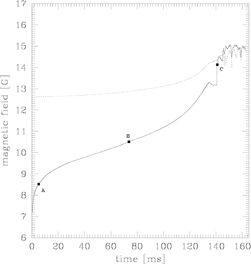
Figure 5: Time evolution of poloidal and toroidal fields at ($r$, $\theta$) = (100 km, $18^{\circ}$) for model H10. The dotted and solid lines correspond to the poloidal and toroidal components, respectively.

The amplification of magnetic field is one of the most important issues in this study. In Fig. 5 we show the time evolutions of magnetic field for models H10. It can be seen that the initially negligible toroidal field is amplified up to values comparable to the poloidal field which has also grown by about four orders of magnitude from its initial strength. It is important to know what process amplifies the magnetic field so greatly. The compression of frozen-in field can amplify the magnetic field. The core contracts from the initial radius, $\sim 10^{8}$ cm, to the final radius some $10^{6}$cm. Hence, the field expected to grow by nearly four orders of magnitude by this process alone. Other possible agencies for field-amplification are the field-wrapping by differential rotation (Meier et al., 1976) and the magnetorotational instability (MRI) (Balbus & Hawley, 1991; Akiyama et al., 2003).

The maximum poloidal field in model H10 grows from $\sim 10^{12}$ to $\sim 10^{16}$ G. The amplitude of the poloidal field-growth, four orders of magnitude, is common to all models, and is just the value expected for the field-compression. This implies the poloidal field is amplified almost entirely by the compression and it does not seen that any instabilities play an important role in our models.

For the toroidal field, we make an estimate for the field-growth rates by field-wrapping and the compression separately. The field wrapping is a process which produces toroidal field from poloidal field by differential rotation. We can estimate this rate by extracting from the $\phi$-component of r.h.s. of Eq. (4) the terms which include rotation velocity and poloidal field;

$$\Biggl{(}\frac{\partial B_{\phi}}{\partial t}\Biggr{)}_{wrap}=\frac{1}{r}\Biggl{[}\frac{\partial(rv_{\phi}B_{r})}{\partial r}+\frac{\partial(v_{\phi}B_{\theta})}{\partial\theta}\Biggr{]}\equiv\alpha.$$ (17)

For the compression, we extract the terms which include $v_{r}$, $v_{\theta}$ and $B_{\phi}$ from the $\phi$ component of r.h.s. of Eq. (4) as:

$$\Biggl{(}\frac{\partial B_{\phi}}{\partial t}\Biggr{)}_{comp}=-\frac{1}{r}\Biggl{[}\frac{\partial(rv_{r}B_{\phi})}{\partial r}+\frac{\partial(v_{\theta}B_{\phi})}{\partial\theta}\Biggr{]}\equiv\beta.$$ (18)

We roughly divide the time evolutions into four phases in terms of the toroidal field-amplification as shown in Fig. 5. For model H10, for example, the first phase is a period from 0 ms to about 10 ms, which shows a first steep gradient in the evolution of maximum fields and includes point A. The second phase is a period from about 10 ms to 140 ms, which corresponds to a gentle growth and contains point B. The third phase continues from about 140 ms to 142 ms, where the second steep gradient appears and point C is representative. This phase corresponds to the period just after the bounce in Fig. 2. The last phase is the period from about 142 ms to the end, which shows a rather chaotic evolution. The growth rates $\alpha$, $\beta$ are presented in Table 3. During the first and second phases, the field-wrapping dominates the compression. During the third phase, on the contrary, the compression becomes dominant over the wrapping which, however, still plays an important role. At the end of the third phase, the ratio of magnetic pressure to matter pressure reaches almost unity and magnetic force begins to play an important role. After the third phase, the maximum toroidal field shows oscillations and grows very slowly. In facts, the growth rates $\alpha$ and $\beta$ also oscillate and are responsible for the oscillating field evolutions. We stop our computations at about 160 - 190 ms when the shock wave reaches 800 km for exploding models.

While the above feature of field evolution is common to all models, the final strength of resulting fields vary from model to model. As shown in Table 2, the final magnetic energy as a result of amplifications is larger in models C’s and Q’s than in model H10 though they have the same initial magnetic energy. This is simply because the initial fields of models C’s and Q’s are more centrally concentrated compared to model H10. Since the field amplification occurs in the vicinity of the boundary between the inner and outer cores, concentrated fields are advantageous. This then causes more energetic explosions in the initially axially-concentrated field models. In the quadrapole-like field models, the explosion energy is rather small since the amplification region is smaller and contains smaller mass.

3.3 Models with Initially Weak Fields

Models with initially weak fields do not lead to substantial matter ejection no matter what the initial configuration is adopted. In fact, there appears no region where magnetic pressure is comparable to matter pressure through the whole simulations. It seems that MRI-like instability do not occur in our models, which would lead to the exponential growth of fields. As a result, magnetic fields do not evolve large enough to affect dynamics.

4 Discussion and Conclusion

We have done two-dimensional MHD simulations on core-collapse of massive stars for several initial configurations of magnetic field, which include the uniform and axially-concentrated fields, quadrapole-like field and toroidal fields. Different differential rotations have been considered. We mainly focus on the systematic trends among the models.

Since it is impossible at the moment to observe magnetic fields of presupernova stars, we have treated the field strength and configuration as free parameters in this study. Nevertheless, there are some suggestions from the theoretical studies of stellar evolutions (Heger et al., 2003) although they are admittedly uncertain. For example, the toroidal field may be dominant prior to core-collapse, since the differential rotation is inevitably produced as the core contracts in the quasi-static evolutionary stages. It may be also possible that magnetic field may be centrally concentrated if it traces the density profile. Bearing these suggestions in mind, we have studied the effect of poloidal fields and toroidal fields separately and have also adopted centrally-concentrated field configurations.

In the models with axially-concentrated fields the explosion energy is about 1.5 times as large as that of the model with uniform field if the initial ratio of magnetic energy to gravitational energy is identical. Although we have not calculated a model with more small values of $r_{0}$ and $\varpi_{0}$, it is expected that larger degrees of field concentration or differential rotation will give more energetic explosions. According to Meier et al. (1976), there may exist a threshold in the initial strength of magnetic field for the MHD explosion. We expect that the parallel field concentration will lower the threshold if any at all.

Our models with quadrapole-like fields give tightly collimated and very high velocity but less energetic explosions. The velocity becomes about half the light speed. This result might have some implications for gamma-ray bursts (GRB). In the paper of Wheeler et al. (2002), they argued a scenario, in which a “fast toroidal jet” is produced first but does not lead to the MHD explosion, and a black hole is formed. Then the second even faster, highly relativistic jet is supposed to be produced from the black hole and interacts with the first slower jet to give GRB. The jets in model Q’s might be something like “fast toroidal jet” in their scenario, since our jet is fast and toroidal-field dominant, and carries only a small part of core mass so that there would remain plenty of energy to produce the second highly relativistic jet. Our jet will be able to sweep out baryons on its way, which will then help the second jet be accelerated to an extremely relativistic velocity. Note that, however, their “fast toroidal jet” is generated in proto-pulsar phase and the origin is different from our jet. The present mesh resolution is not sufficient to properly treat a tight collimation, and numerical simulations with finer angular mesh are needed. Special relativity should be also included.

Our results for the quadrapole-like fields look quite different from that of Ardeljan et al. (2004) in which the almost same field configuration is employed. Their simulation resulted in more energetic explosion, $0.6\times 10^{51}$erg, than ours and matter is ejected more strongly in the direction parallel to the equatorial plane. They employed a 2D implicit Lagrangian code with a parametric EOS, neutrino losses and iron dissociations by introducing approximate formulae. The main difference is the way to set the initial magnetic field. They ’turned on’ the quadrapole-like field well after the collapse of the core, when the toroidal fields have already grown in our models. What is more, as they set the initial ratio of magnetic energy to gravitational energy to be $10^{-6}$, the growth of magnetic field is further delayed. We think this is the reason for apparent difference.

Akiyama et al. (2003) claimed that MRI is likely to grow in the postbounce core (see, however, Fryer & Warren, 2004). In the present simulations, as mentioned already MRI-like field-amplification process is not found. In particular, the initial weak fields in models H10w, C5w, Q5w, T5w do not develop so mach as to influence dynamics. This is again at odds with the results of Ardeljan et al. (2004). We suppose that this is mainly due to the spacial resolution of our simulations. It should be note that since the toroidal fields are highly likely to be dominant in the post bounce core and MRI operates also non-axisymmerically, 3D simulations will be important in considering MRI. We are already undertaking three dimensional MHD simulations with high resolution scheme (Sawai et al., 2005), and results will be presented elsewhere.

If MRI grows efficiently form weak seed fields as some authors claimed, the normal supernova may be also explained by the MHD process (Wheeler et al., 2002). Then we may have to worry about how to reduce the magnetic fields by the time the pulsar is observed, since otherwise the magnetar would be a common product. These are important issues for the future work.

Table 1: Magnetic Field and Differential Rotation for Initial Models

Model	$|E_{m}/W|$ [%]	$|T/W|$ [%]	$B_{i}$ [G]	$\Omega_{i}$ [rad/s]	$r_{0}$ or $\varpi_{0}$ [km]	$R_{0}$ [km]
R10	0.0	0.5	0.0	0.0	-	-
H10	0.5	0.5	$4.1\times 10^{12}$	3.9	$\infty$	1000
C5	0.5	0.5	$1.4\times 10^{13}$	7.0	500	500
C10	0.5	0.5	$8.2\times 10^{12}$	3.9	1000	1000
Q3	0.5	0.5	$8.4\times 10^{12}$	$1.3\times 10$	-	300
Q5	0.5	0.5	$8.4\times 10^{12}$	7.0	-	500
Q10	0.5	0.5	$8.4\times 10^{12}$	3.9	-	1000
T3	0.5	0.5	$5.1\times 10^{13}$	$1.3\times 10$	300	300
T5	0.5	0.5	$2.6\times 10^{13}$	7.0	500	500
T10	0.5	0.5	$1.1\times 10^{13}$	3.9	1000	1000
H10w	10-8	0.5	$5.8\times 10^{8}$	3.9	$\infty$	1000
C5w	10-8	0.5	$2.0\times 10^{9}$	7.0	500	500
Q5w	10-8	0.5	$1.2\times 10^{9}$	7.0	-	500
T5w	10-8	0.5	$3.6\times 10^{9}$	7.0	500	500

Table 2: Key Parameters for All Models

Model	$M_{IC}$	$|E_{m}/W|_{b}$	$|T/W|_{b}$	$B_{b},max$	$\Omega_{b},max$	$|E_{m}/W|_{fin}$	$|T/W|_{fin}$	$B_{fin,max}$	$\Omega_{fin,max}$	$v_{fin,max}$	$E_{exp}$	$M_{ej}$	$\Delta\theta$	$f_{shock}$
R10	0.82	0.0	$1.0\times 10$	0.0	$7.9\times 10^{3}$	0.0	6.8	0.0	$7.5\times 10^{3}$	$4.9\times 10^{8}$	0.12	0.013	180	0.98
H10	0.82	0.15	8.9	$2.0\times 10^{16}$	$1.0\times 10^{4}$	0.62	4.0	$2.2\times 10^{16}$	$5.3\times 10^{3}$	$4.6\times 10^{9}$	1.6	0.18	42	1.5
C5	0.82	0.70	9.1	$1.6\times 10^{16}$	$8.0\times 10^{3}$	1.3	4.4	$6.5\times 10^{16}$	$8.7\times 10^{3}$	$6.3\times 10^{9}$	2.1	0.16	42	2.0
C10	0.81	0.25	8.0	$1.8\times 10^{16}$	$7.3\times 10^{3}$	1.1	3.7	$6.6\times 10^{16}$	$3.3\times 10^{3}$	$6.4\times 10^{9}$	2.3	0.17	54	1.9
Q3	0.89	0.075	$1.1\times 10$	$1.0\times 10^{16}$	$9.8\times 10^{3}$	0.90	6.8	$2.6\times 10^{16}$	$8.3\times 10^{3}$	$9.8\times 10^{9}$	0.24	0.021	6	1.6
Q5	0.83	0.060	$1.0\times 10$	$7.0\times 10^{15}$	$8.0\times 10^{3}$	0.96	5.9	$3.0\times 10^{16}$	$8.5\times 10^{3}$	$5.2\times 10^{9}$	0.26	0.029	12	1.4
Q10	0.81	0.041	9.0	$1.0\times 10^{16}$	$1.1\times 10^{4}$	1.1	5.0	$6.5\times 10^{16}$	$6.8\times 10^{3}$	$1.3\times 10^{10}$	0.59	0.066	24	1.3
T3	0.91	0.58	$1.0\times 10$	$9.0\times 10^{16}$	$4.2\times 10^{3}$	0.52	7.2	$3.3\times 10^{16}$	$2.6\times 10^{4}$	$4.8\times 10^{8}$	0.11	0.012	180	0.93
T5	0.82	0.33	$1.0\times 10$	$7.1\times 10^{16}$	$2.7\times 10^{4}$	0.30	6.8	$1.8\times 10^{16}$	$9.3\times 10^{3}$	$5.4\times 10^{8}$	0.091	0.010	180	0.89
T10	0.81	0.12	8.4	$5.7\times 10^{16}$	$1.8\times 10^{4}$	0.11	5.9	$1.4\times 10^{16}$	$1.1\times 10^{4}$	$6.5\times 10^{8}$	0.14	0.016	180	0.93
H5w	0.80	$2.3\times 10^{-9}$	8.2	$3.5\times 10^{12}$	$8.6\times 10^{3}$	$5.2\times 10^{-7}$	6.1	$5.5\times 10^{13}$	$1.2\times 10^{4}$	$8.8\times 10^{8}$	0.14	0.027	180	1.2
C5w	0.82	$3.2\times 10^{-8}$	$1.0\times 10$	$1.0\times 10^{13}$	$7.9\times 10^{3}$	$5.6\times 10^{-6}$	6.9	$5.4\times 10^{13}$	$9.0\times 10^{3}$	$8.2\times 10^{8}$	0.11	0.018	180	0.95
Q5w	0.82	$1.4\times 10^{-9}$	$1.0\times 10$	$1.5\times 10^{12}$	$7.9\times 10^{3}$	$3.0\times 10^{-7}$	6.9	$6.2\times 10^{12}$	$9.2\times 10^{3}$	$8.0\times 10^{8}$	0.10	0.017	180	0.97
T5w	0.82	$6.8\times 10^{-9}$	$1.0\times 10$	$1.9\times 10^{13}$	$7.9\times 10^{3}$	$6.4\times 10^{-9}$	6.9	$2.7\times 10^{12}$	$9.2\times 10^{3}$	$7.9\times 10^{8}$	0.10	0.017	180	0.97

Note. — $|E_{m}/W|$ : the magnetic energy normalized by the gravitational energy. $|T/W|$ : the rotation energy normalized by the gravitational energy. $B_{i}$ : the initial maximum magnetic field. $\Omega_{i}$ : the initial angular velocity at the center of the core. $r_{0}$ and $\varpi_{0}$ : the parameters which specify the degree of field concentration (see Eqs. (13) and (15)). $R_{0}$ : the parameter which specifies the degree of the differential rotation (see Eq. (16)).

Note. — $M_{IC}$ : the inner core mass at bounce in unit of $M_{\odot}$. $\rho_{c}$ : the central density at bounce in $10^{14}$ g/cm³. The ratios $|E_{m}/W|$ and $|T/W|$ are given in percentage. $B_{max}$ : the maximum magnetic field in G. $\Omega_{max}$ : the maximum angular velocity in rad/s. $v_{max}$ : the maximum positive radial velocity in cm/s. $E_{exp}$ : the explosion energy in $10^{51}$erg. $M_{ej}$ : the ejected mass in $M_{\odot}$. $\Delta\theta$ : the opening angle of the induced jet in degree (see the footnote in §3 for the definition). $f_{shock}$ : the aspect ratio. For all parameters, the subscripts “$b$” and “$fin$” denote the values at bounce and those at the end of calculations, respectively.

Table 3: The Field Growth Rate in Model H10

Point	$t_{eva}$ [ms]	$|B_{\phi}|$ [G]	$|\alpha|$ [G/s]	$|\beta|$ [G/s]
A	5.2	$3.2\times 10^{8}$	$5\times 10^{11}$	$8\times 10^{8}$
B	73.7	$3.2\times 10^{10}$	$2\times 10^{12}$	$3\times 10^{11}$
C	140.9	$1.3\times 10^{14}$	$4\times 10^{16}$	$1\times 10^{17}$

References

- Akiyama et al. (2003) Akiyama, S., Wheeler, J. C., Meier, D. L., & Lichtenstadt, I. 2003, ApJ, 584, 954
- Ardeljan et al. (1998) Ardeljan, N. V., Bisnovatyi-Kogan, G. S., & Moiseenko S. G. 1998, LPN, 506, 145A
- Ardeljan et al. (2000) Ardeljan, N. V., Bisnovatyi-Kogan, G. S., & Moiseenko S. G. 2000, Astron. Astrophys. , 355, 1181
- Ardeljan et al. (2004) Ardeljan, N. V., Bisnovatyi-Kogan, G. S., & Moiseenko S. G. 2004, submitted to the MNRAS
- Balbus & Hawley (1991) Balbus, S. A., & Hawley, J. F. 1991, ApJ, 376, 214
- Bisnovatyi-Kogan et al. (1975) Bisnovatyi-Kogan, G. S., Popov, YU. P., & Samochin, A. A. 1975, Ap&SS, 41, 287B
- Blondin et al. (2003) Blondin, J. M., Mezzacappa, A., & DeMarino, C. 2003, ApJ, 584, 971
- Buras et al. (2003) Buras, R., Janka, H. -T., & Kifonidis, K. 2003, Phys. Rev. Lett., 90, 241101
- Duncan & Thompson (1992) Duncan, R. C., & Thompson, C. 1992, ApJ, 392, L9
- Foglizzo & Tagger (2000) Foglizzo, T., & Tagger, M. 2000, Astron. Astrophys., 363, 174
- Fryer & Warren (2004) Fryer, C. L., & Warren, M. S. 2004, ApJ, 601, 391
- Heger et al. (2003) Heger, A., Woosley, S. E., Langer, N., & Spruit, H. C. 2003, Proc. IAU 215 “Stellar Rotation”
- Janka et al. (2005) Janka, H. -T., Buras, R., Kitaura Joyanes, F. S., Marek, A., Rampp, M., & Scheck, L. 2005, Proc. “Nuclei in the cosmos 8”, to appear in Nucl. Phys. A, astro-ph/0411347
- Kotake et al. (2003) Kotake, K., Yamada, S., & Sato, K. 2003, ApJ, 595, 304
- Kotake et al. (2004) Kotake, K., Sawai, H., Yamada, S., & Sato, K. 2004, ApJ, 608, 391
- LeBlanc & Wilson (1970) LeBlanc, J. M., & Wilson, J. R. 1970, ApJ, 161, 541
- Leonard et al. (2000) Leonard, D. C., Filippenko, A. V., Barth, A. J., & Matheson, T. 2000, ApJ, 536, 239
- Liebendörfer et al. (2001) Liebendörfer, M., Mezzacappa, A., Thielemann, F. -K., Messer, O. E. B., Hix, W. R., & Bruenn, S. W. 2001, Phys. Rev. D, 63, 103004
- Liebendörfer et al. (2004) Liebendörfer, M., Rampp, M., Janka, H.-T., & Mezzacappa, A. 2004, ApJin press, astro-ph/0310662
- Meier et al. (1976) Meier, D. L., Epstein, R. I., Arnett, W. D., & Schramm, D. N. 1976, ApJ, 204, 869
- Müller & Hillebrandt (1979) Müller, E., & Hillebrandt, W. 1979, Astron. Astrophys., 80, 147
- Ohnishi (1983) Ohnishi, T. 1983, Tech. Rep. Inst. At. En. Kyoto Univ. No.198
- Rampp & Janka (2000) Rampp, M., & Janka, H. -T. 2000, ApJ, 539, L33
- Sawai et al. (2005) Sawai, H., Kotake, K. & Yamada, S. 2005, now in preparation
- Shimizu et al. (2001) Shimizu, T. M., Ebisuzaki, T., Sato, K., & Yamada, S. 2001, ApJ, 552, 756
- Stone & Norman (1992) Stone, J. M., & Norman M. L. 1992, ApJS, 80, 791
- Sumiyoshi et al. (2004) Sumiyoshi, K., Suzuki, H., Yamada, S., & Toki, H. 2004, Nucl. Phys., A730, 227
- Symbalisty (1984) Symbalisty, E. M. D. 1984, ApJ, 285, 729
- Takahara & Sato (1984) Takahara, M. & Sato, K. 1984, Prog. Theor. Phys., 71, 524
- Takiwaki et al. (2004) Takiwaki, T., Kotake, K., Nagataki, S., & Sato, K. 2004, ApJ, 616, 1086
- Thompson & Duncan (1996) Thompson, C., & Duncan, R. C. 1996, ApJ, 473, 322
- Thompson et al. (2003) Thompson, T. A., Burrows, A., & Pinto, P. A. 2003, ApJ, 592, 434
- Walder et al. (2005) Walder, R., Burrows, A., Ott, C. D., Livne, E., Jarrah, M. 2005, submitted to ApJ, astro-ph/0412187
- Wang et al. (1996) Wang, L., Wheeler, J. C., Li, Z., & Clocchiatti, A. 1996, ApJ, 467, 435
- Wheeler et al. (2000) Wheeler, J. C., Yi, I., Höflich, P., & Wang, L. 2000, ApJ, 537, 810
- Wheeler et al. (2002) Wheeler, J. C., Meier, D. L., & Wilson, J. R. 2002, ApJ, 568, 807
- Woosley (1995) Woosley, S. E. 1995, private communication
- Yamada & Sato (1994) Yamada, S., & Sato, K. 1994, ApJ, 434, 268
- Yamada & Sawai (2004) Yamada, S., & Sawai, H. 2004, ApJ, 608, 907
- Yamasaki & Yamada (2005) Yamasaki, T., & Yamada, S. 2005, submitted to ApJ, astro-ph/0412625