The Low-Redshift Ly$\alpha$ Forest toward PKS 0405–123^1,2

Abstract

We present results for Ly$\alpha$ forest and metal absorbers from $\sim 7$ km s^-1 resolution data from the Space Telescope Imaging Spectrograph for the QSO PKS 0405–123 ($z=0.574$, $V=14.9$). We analyze two samples of low redshift Ly$\alpha$ forest lines, a sample of strong Ly$\alpha$ lines and a sample of weak ones. The strong-line sample consists of 60 Ly$\alpha$ absorbers detected at 4.0$\sigma$ significance with column density $\log\mbox{$N_{HI}$}\geq 13.3$ over $0.002<z<0.423$; the sample of weak lines contains 44 absorbers with a column density limit of $\log\mbox{$N_{HI}$}\geq 13.1$ over $0.020<z<0.234$. Seven of the Ly$\alpha$ absorbers show metal absorption lines. Notably, all of these metal systems appear to have associated O VI absorption, but the O VI is often offset in velocity from the Ly$\alpha$ lines. We do not distinguish between metal and Ly$\alpha$-only systems in the following analysis, and use simulated spectra to aid in the interpretation of results. The Doppler parameter distribution for the strong sample has $\langle b\rangle=47\pm 22$ km s^-1. For the weak sample, $\langle b\rangle=44\pm 21$ km s^-1. Line blending and signal-to-noise effects likely inflate the Doppler parameters. The redshift density is consistent with previous, lower resolution measurements for $\log\mbox{$N_{HI}$}\geq 14.0$. For absorbers with $13.1<\log\mbox{$N_{HI}$}<14.0$, we find results consistent with previous high resolution studies for $z<0.127$ but an overdensity of $\sim 0.2-0.3$ dex at $0.127<z<0.234$, which we believe arises from cosmic variance. We find Ly$\alpha$-Ly$\alpha$ clustering in our sample on a scale of $\Delta v\leq 250$ km s^-1 for $\log\mbox{$N_{HI}$}\geq 13.3$, which is consistent in strength and velocity scale with a numerical model of structure evolution. There is a void in the strong absorber sample at $0.0320<z<0.0814$ with probability of occurrence from a random redshift distribution of $P<0.0004$. We detect line-of-sight velocity correlations of up to 250 km s^-1 between Ly$\alpha$ absorbers and 39 galaxies at $z<0.43$ in the field out to transverse distances covering up to 1.6 $h^{-1}_{70}$ Mpc in the local frame. The Ly$\alpha$-galaxy two point correlation function is significant out to $\Delta v<250$ km s^-1 and grows with minimum absorber H I column density, with the strongest signal for $\log\mbox{$N_{HI}$}{\gtrsim}13.5-14.0$ absorbers. The strength is similar to that of the galaxy-galaxy correlation for galaxies of the same mean luminosity as our sample, which implies that such Ly$\alpha$ absorbers have masses $\log M/M_{\odot}=11.3^{+1.0}_{-0.6}$. The correlation becomes insignificant for a sample limited to $13.1\leq\log\mbox{$N_{HI}$}<14.3$. Including lower column density systems in the sample shows correlations only out to $\Delta v<125$ km s^-1, as would be expected for smaller density perturbations. We find a correlation between local galaxy counts and local summed H I column density, with peak significance on scales of $4000-6000$ km s^-1 and the probability of occurrence from uncorrelated data of $P=0.0009$ . Based on galaxy counts in the field, we predict regions of low H I column density at $z\approx 0.45$ and high values at $z\approx 0.43$ and $z\approx 0.51$ toward PKS 0405–123. Finally, we present column densities for a number of Galactic species.

1 Introduction

An explanation for the Ly$\alpha$ forest is among the most impressive successes of CDM structure formation models (e.g. Miralda-Escudé et al., 1996; Davé et al., 1999, 2001; Davé & Tripp, 2001), with CDM simulations naturally reproducing the rich Ly$\alpha$ absorption seen in QSO spectra. At $z<1.5$, where Ly$\alpha$ must be observed from space, a database has only slowly accumulated for the Ly$\alpha$ forest, both for absorber statistics and for comparisons with the nearby galaxy distribution. The Ly$\alpha$ forest redshift density is known for higher equivalent widths (rest equivalent width $W_{0}>0.200$ Å, Weymann et al., 1998), but currently available samples are much smaller for weaker Ly$\alpha$ absorbers with $W_{0}\ll 0.200$ Å (e.g. Tripp et al., 1998; Penton et al., 2004; Richter et al., 2004; Sembach et al., 2004). The H I column density distributions at low and high redshift appear consistent with each other (Penton et al.), whereas clustering in the Ly$\alpha$ forest at low $z$ is expected (Davé et al., 1999) but has been challenging to detect. Among recent studies, Janknecht et al. (2002) found no evidence for clustering via the two point correlation function for velocity scales $\Delta v<1000$ km s^-1 for a sample of 235 Ly$\alpha$ forest lines over column densities $13.1<\log\mbox{$N_{HI}$}<16.4$ at redshifts $0.9<z<1.7$. However, Penton et al. found a $5.3\sigma$ signal for clustering at $\Delta v<190$ km s^-1 (and 7.2 $\sigma$ for $\Delta v<260$ km s^-1) at $0.002<z<0.069$ for 187 Ly$\alpha$ absorbers with rest equivalent width $W_{0}>0.065$ Å  ($\log\mbox{$N_{HI}$}{\gtrsim}13.1$). The nature of clustering in the Ly$\alpha$ forest is thus still a matter of active investigation, as is the redshift density of low column density absorbers.

Numerical models for the Ly$\alpha$ forest have led to an interpretation for Ly$\alpha$ absorbers in which weak lines are opacity fluctuations tracing the underlying dark matter distribution, while stronger systems ($N(\mbox{{H~{}I}}){\gtrsim}10^{16-17}$cm^-2) represent higher overdensity regions and are often affiliated with galaxies. Thus Ly$\alpha$ absorbers in a single quasar spectrum probe density perturbations across a wide range of scales, from voids to groups of galaxies. Metal absorbers provide complementary information about the abundances, kinematics and ionization conditions near galaxy halos and in the intergalactic medium (e.g. Bowen et al., 1995; Davé et al., 1998; Chen & Prochaska, 2000; Tripp et al., 2001, 2002, 2005; Rosenberg et al., 2003; Shull et al., 2003; Tumlinson et al., 2005; Keeney et al., 2005; Jenkins et al., 2005). Metal systems also give indications about the strength of feedback from supernovae in galaxies, and, in the case of O VI absorbers, can contain large reservoirs of baryons at both low and high redshift, e.g. Tripp et al. (2000); Savage et al. (2002); Carswell, Schaye, & Kim (2002); Simcoe, Sargent, & Rauch (2004) (cf. Pieri & Haehnelt, 2004).

Therefore, understanding the evolution of the intergalactic medium (IGM) near galaxies from high to low redshifts will help constrain feedback processes that impact the formation of galaxies and their surrounding intragroup and intracluster media. At higher redshift, Adelberger et al. (2003) found that the IGM at $z\sim 3$ contains more than the average amount of H I at $1{\lesssim}r{\lesssim}5\,h^{-1}$ comoving Mpc from LBGs. A strong correlation between LBGs and metals (particularly CIV) in the IGM was also noted, indicating a link between LBGs and CIV absorbers. They suggested that the decrease in H I close to LBGs and the metal enrichment around LBGs may be the result of supernovae-driven winds; the topic currently remains an area of active investigation.

At $z\leq 0.5$, galaxies are relatively easy to identify, but the Ly$\alpha$ forest itself is sparse. In the nearby universe ($z<0.3$), many authors have found making a one-to-one association between galaxies and Ly$\alpha$ absorbers to be a challenge. Nevertheless, current evidence indicates that Ly$\alpha$ absorbers and galaxies cluster, though less strongly than the galaxy-galaxy correlation (Morris et al., 1993; Stocke et al., 1995; Tripp et al., 1998; Impey, Petry, & Flint, 1999; Penton, Stocke, & Shull, 2002). At even lower redshifts, Bowen et al. (2002) found 30 Ly$\alpha$ absorbers with the Space Telescope Imaging Spectrograph (STIS) around 8 galaxies, with column densities $\log N_{HI}\geq 13.0$; sight lines passing within $\sim 200\,h^{-1}$ kpc of a galaxy almost always show H I absorption. The absorption tends to extend over 300-900 km s^-1, making a one-to-one correspondence between an absorption system and any particular galaxy difficult, though summing the absorption over $\Delta v\sim 1000$ km s^-1 produces a correlation of H I strength with proximity to individual galaxies as found at $0.1{\lesssim}z{\lesssim}1$ by Chen et al. (2001, and references therein). The correlation of $N_{HI}$ with proximity to regions of high galaxy density noted by Bowen et al. is likely related to the correlation seen by Adelberger et al. However, the quantitative evolution of such correlations tracks overdensities associated with typical Ly$\alpha$ absorbers of varying strengths, so that at $z{\lesssim}1$, stronger lines are predicted to arise in regions of high galaxy density (e.g. Davé et al., 1999; McDonald, Miralda-Escudé, & Cen, 2002).

A more direct correlation arises between the sum of the H I column density over intervals of $\sim 1000$ km s^-1 and the local volume density  of galaxies brighter than $M_{B}=-17.5$ (Bowen et al., 2002) within $\sim 2\,h^{-1}$ Mpc of the QSO sight line, qualitatively similar to the Adelberger et al. results over $5\,h^{-1}$ comoving Mpc. The H I column density – galaxy volume density correlation is intriguing, because the Ly$\alpha$ forest at $z\sim 3$ and $z<1$ appears to sample different degrees of overdensities, very possibly due to the expansion of the universe and rapidly falling UV background flux at low redshifts (Davé et al., 1999). A key to understanding the correlation would rely on acquiring high-quality observations of the Ly$\alpha$ forest – galaxy correlation over $0.1<z<1$ to bridge the gap between the Bowen et al. and Adelberger et al. results.

In this paper, we address questions concerning the redshift density of low redshift Ly$\alpha$ absorbers, especially low column density systems, their correlations and their relationship to nearby galaxies by obtaining high resolution UV spectra of the QSO PKS0405–12 ($V=14.9$, $z=0.574$) and comparing them with a galaxy sample drawn from the literature and from ground-based observations presented here. It is one of the brightest QSOs in the sky, and illuminates a much longer path in the Ly$\alpha$ forest than most of the other QSOs of similar or brighter magnitude. PKS 0405–123 is therefore a prime target for studies of the low $z$ Ly$\alpha$ forest and metal absorbers and mid-latitude ($\ell=295^{\rm\,o}$, $b=-42^{\rm\,o}$) studies of Galactic absorption. We use $\sim 7$ km s^-1 resolution STIS data to calculate the Ly$\alpha$ forest redshift density, Doppler parameter, clustering and void statistics, and to cross-correlate the Ly$\alpha$ forest and field galaxy redshifts. In support of the Ly$\alpha$ forest work, we present observations of 42 galaxies from a ground-based survey in the region, and add 31 galaxies from the literature to our sample.

Our observations and data reduction are described in § 2, and we outline the profile fitting method and absorber sample in § 3. The various absorber distribution functions and correlation functions are described in § 5. In § 6, we compare the absorbers against a galaxy sample. We discuss the results in § 7, and summarize our conclusions in § 8. We adopt a cosmology of $H_{0}=70$ km s^-1 Mpc^-1, $\Omega=0.3$, $\Lambda=0.7$ throughout this work.

2 Observations and reductions

Our principal data are from the Hubble Space Telescope (HST) plus STIS, using guaranteed time from Program 7576 to the STIS Instrument Definition Team. We also use archival HST spectra of PKS 0405–123 and ground-based galaxy images and redshifts in a supportive role.

2.1 STIS spectra

PKS 0405–123 was observed with HST and STIS using grating E140M for ten orbits (27208 sec) on 1999 Jan 24 and 1999 Mar 7. We used the $0.2^{\prime\prime}\times 0.06^{\prime\prime}$ slit for maximal spectral purity. For this setup, the STIS Instrument Handbook gives $R=45800$.

The data were processed with calstis, including correction for scattered light and spectral extraction, using STIS IDT team software at Goddard Space Flight Center. After merging the spectral orders, we constructed a continuum using a combination of routines from automated autovp (Davé, 1997) and interactive line_norm by D. Lindler, because the regions around emission lines were best done with manual fitting. The final spectrum has a signal-to-noise ratio per $\sim 3.2$ km s^-1 pixel in the Ly$\alpha$ forest of 4 to 7 except for small dips at the ends of orders. Redward of 1581 Å, we lose coverage of $\Delta z=0.0035$ for Ly$\alpha$ due to six inter-order gaps. The signal to noise ratio is $\sim 5-10$ per $\sim 2$ pixel resolution element in the Ly$\alpha$ forest.

2.2 HST archival spectra

We retrieved and summed archival HST spectra from the Faint Object Spectrograph (FOS, Proposal 1025, gratings G130H, G190H and G270H) Goddard High Resolution Spectrograph (GHRS, Proposal 6712, gratings G160M and G200M) and STIS (Proposal 7290, grating G230M), to provide consistency checks for wavelengths covered by our E140M data and to provide complementary Ly$\alpha$ forest and metal line information outside of the E140M spectral range.

2.3 Ground-based galaxy images and spectra

Direct images in Gunn $r$ and multi-object spectroscopic observations of galaxies in the PKS 0405–123 field were made on 1995 Jan 2 UT at the Canada-France Hawaii Telescope (CFHT), using the MOS spectrograph, the O300 grism, and the z5 band-limiting filter. The data are part a survey of the environments of bright AGN Ellingson & Yee (1994). The stellar point spread function in the final stacked $10.2\times 9.8$ arcmin² MOS direct image is 2.0 arcsec, and the limiting magnitude for extended sources is $r\approx 22.6$ ($r=23.3$ for point sources). There are 175 galaxies with $r<22.5$, and 258 with $r<23.5$. The spectral range was 5300–7000 Å, with a resolution of about 12 Å. Object selection and aperture plate design were carried out using the observation and reduction techniques described in Yee, Ellingson & Carlberg (1996). The band-limiting filter yielded 78 apertures on a single aperture mask spanning a region approximately 8 by 4 arcminutes around the quasar. Slits were designed to be 1.5 arcseconds wide and a minimum of 10 arcseconds long. Three one-hour integrations were taken with this mask. PKS 0405–123 was targeted, preventing additional apertures from being placed with about 5 arcseconds of the quasar. The total area covered in the data presented here is nearly three times that of Ellingson & Yee, and the spectral resolution is about double.

From these data, spectra of galaxies were identified via cross-correlation with a series of galaxy templates, and galaxy magnitudes in Gunn $r$ were derived from the MOS images used to create the aperture masks. Uncertainties in the photometry are about 0.1 mag. Redshifts for objects up to $r\approx 23$ were measured, with most of the fainter objects identified via emission lines. The spectroscopic completeness is difficult to judge accurately because some of the objects are stars and due to positional selection constraints from the multi-slit spectroscopic setup. For $r<22.0$ we have spectroscopic redshifts from our CFHT data for 46 of 206 objects (17%), of which 126 are more extended than our stellar point spread function. The targets were selected from an 8 arcmin square field centered on PKS 0405–123. The limited spectral range provided somewhat higher success rates for objects with $0.35<z<0.7$, but redshifts for galaxies between 0.1 and 0.35 were also identified (see Yee, Ellingson & Carlberg for quantitative details). Also, because of the limited wavelength coverage, many of the redshifts rely on a single line identification. Uncertainties in galaxy redshifts are estimated to be about 100 km s^-1 in the rest frame, based on extensive redundant observations carried with MOS in this and other surveys, with a possible systematic component less than about 30 km s^-1.

To compare our results with those of Ellingson & Yee (1994) our new galaxies for which we have redshifts have average $\langle r\rangle=21.4\pm 0.9$ vs. $\langle r\rangle=21.1\pm 0.8$ from Ellingson & Yee and Spinrad et al. (1993) (excluding the uncertain magnitude of galaxy 309). The new CFHT data include 36 emission and six absorption galaxies, with the faintest redshift for $r=23.4$, whereas the sample from the literature includes 19 emission, ten absorption and two other galaxies with the faintest redshift for $r=22.5$. Three of the galaxies from the literature, [EY94] 231 and 398, and [EY93] 309, were re-observed spectroscopically. Results were consistent for the latter two objects. We confirm a redshift of $z=0.5696$ for [EY94] 231, which coincides with [EY93] 232. Overall, the galaxy list here contains redshifts for 44% of the 87 galaxies in the MOS field to $r<21.5$ compared to 23% for the smaller area survey of Ellingson & Yee, and 39% of 175 galaxies to $r<22.5$ compared to 18% for the previous work.

3 Absorption line selection

The entire STIS E140M spectrum of PKS0405–123 is shown in Figure 1. We selected absorption features from the summed STIS E140M data at the $4.0\sigma$ significance level with a Gaussian filter based on an autovp routine, with half-widths of 8, 12, 16, and 20 pixels. We then confirmed significant features with a simple equivalent width significance criterion based on a 4$\sigma$ threshold for contiguous pixels below the continuum, summed in quadrature. Whenever possible and necessary, we confirmed spectral features in the STIS E140M data with the archival FOS and GHRS data. The STIS echelle spectra have substantially better spectral resolution and wavelength coverage, so we did not sum together data from the different instruments, and only used the STIS E140M data for quantitative analysis of the Ly$\alpha$ forest.

G. Williger profile-fitted the data with vpfit (Webb, 1987) using Voigt profiles convolved with the STIS line spread function (LSF) taken from the STIS Instrument Handbook. Multiple transitions (e.g. Ly$\alpha$, $\beta$, $\gamma$) are used for simultaneous fits whenever they improve constraints on column densities and Doppler parameters. For comparison, R. Carswell made an independent fit, though some of the higher column density systems were not fitted as far down the Lyman series as done by Williger. The two profile fits were largely consistent. We allowed for an offset uncertainty in the continuum for some of the fits, as we deemed necessary for accurate error estimates. In addition to H I lines, we find and list, for completeness, profile fits or column density limits (from the apparent optical depth method, Savage & Sembach, 1991) for a number of Galactic and intervening metal absorption lines. Our search for intervening metal lines included archival HST GHRS G200M and STIS G230M data. The intervening metal absorber redshifts will be considered with respect to galaxies in the region. However, a further detailed study of them is beyond the scope of this paper; they are discussed in Prochaska et al. (2004). Intervening systems with metals include $z=$ 0.09180, 0.09658, 0.167, 0.1829, 0.3608, 0.3616, 0.3633, and 0.4951. We did not find significant O VI absorption at $z=0.1825$, in accord with the result of Prochaska et al. (2004), and do not include it in any of our analysis. Chen & Prochaska (2000) have studied the abundances and ionization state of the $z=0.167$ system, and Prochaska et al. have determined its H I column density from FUSE data, which we adopt.

Extragalactic metal systems. (Prochaska et al., 2004) have analyzed the metal absorbers in the PKS0405–123 spectrum in detail including the systems at $z=$ 0.09180, 0.09658, 0.167, 0.1829, 0.3608, 0.3633, and 0.4951. We find evidence for an additional O VI doublet at $z=0.3616$, with rest equivalent widths of $46\pm 15$ mÅ and $44\pm 11$ mÅ for the $\lambda 1031$ and $\lambda 1037$ components, respectively, using the method of Sembach & Savage (1992). It is interesting to note that all of these metal systems show O VI. However, in many cases there are substantial offsets in velocity between the O VI centroid and the H I velocity centroid. Based on our Voigt-profile fitting centroids, we find that the O VI at $z=0.16701$ is offset by $-34$ km s^-1 from the corresponding H I centroid, O VI at $z=0.18292$ is offset by +51 km s^-1, and O VI at $z=0.36156$ is offset by +168 km s^-1. Similar differences in O VI and H I velocity centroids have been reported in other sight lines (e.g. Tripp et al., 2000, 2001; Richter et al., 2004; Sembach et al., 2004). These velocity offsets are too large to attribute to measurement errors. Instead, they indicate that the absorption systems are multiphase entities in which the O VI and H I absorption arises, at least in part, in different places.

Galactic absorption. We find Galactic absorption from H I, C I, C II, C II^∗, C IV; N I, O I, Al II, Si II, Si II^∗, Si III, Si IV, P II, S II, S III, Fe II, Ni II. All Galactic absorption is at $-73<v<32$ km s^-1, so there is no evidence for any high-velocity clouds. A more detailed analysis of these ions is also beyond the scope of this paper. A complete list of absorber profile fitting parameters is in Table 1.

4 Simulated spectra to determine detection probabilities

To give us a clearer picture of our Ly$\alpha$ line detection probability as a function of s/n ratio and Doppler parameter, we analyzed 1440 simulated Ly$\alpha$ lines to determine the 80% line detection probability. The simulated lines were generated using the STIS LSF and a grid of values in Doppler parameter $b$ ($17.5\pm 0.3$, $24.7\pm 0.3$, $35.0\pm 0.3$ km s^-1) and in s/n ratio per pixel (4,7,12). The input log $N_{HI}$  values range over the intervals 12.85–13.35, 12.60–13.10 and 12.31–12.80 respective to the s/n ratio grid. The simulated spectra were continuum-normalized, so any errors, systematic or random, involving continuum fitting would not be reflected in the subsequent analysis. We calculated statistics comparing the line parameters for simulated lines which were successfully recovered vs. the input values. Results for the various combinations of input s/n ratio and Doppler parameter are shown in Tables 2 and 3. The mean recovered measured Doppler parameters match the mean input values within the mean of the profile fitting errors. The same is true for the log H I column densities for input s/n ratio per pixel 12. However, the mean recovered H I column densities are marginally high compared to the mean input values for s/n ratio 7 and are even less in agreement for s/n ratio 4, with a mean difference up to $\Delta\log\mbox{$N_{HI}$}=0.17$ and a mean measured column density error of $\langle\sigma(N(\mbox{{H~{}I}})\rangle=0.09$. The reason for the marginally higher measured H I column densities is because for the weak lines which we considered to probe the 80% detection threshold, noise effectively lowered an absorber’s fitted column density from above to below the detection threshold more often than it increased an absorber’s column density from below to above. Such selective removal biases to higher values the H I column densities for matches between simulated and measured lines. The spurious detection rate is $<0.1$% among all the simulations above the 80% detection probability threshold, and is not considered significant. The boundary of the 80% detection probability threshold can be parametrized by $\log\mbox{$N_{HI}$}=12.870+0.344\log(b/24.7)-1.012\log({\rm snr}/7.)$, where snr is the s/n ratio per pixel.

5 Ly$\alpha$ absorber statistics

In consideration of the $N_{HI}$ sensitivity of the data and to provide a comparison to other studies in the literature, we define two samples based on H I column density: a “strong” one for $\log(N(\mbox{{H~{}I}}))\geq 13.3$ and a “weak” one for $\log(N(\mbox{{H~{}I}}))\geq 13.1$. The strong sample was chosen to take advantage of the minimum s/n ratio over most of the Ly$\alpha$ forest region, while the weak one was chosen to focus on weak absorbers and to be comparable to other high resolution studies. We use the s/n ratio of the data as a function of wavelength, a $4.0\sigma$ significance threshold and a Doppler parameter of $b=40$ km s^-1, which is close to the mean value of $b$ in our data to determine the redshifts corresponding to the two samples. Consequently, the strong sample contains the range $0.002<z<0.423$ and 60 Ly$\alpha$ absorbers, whereas the weak one spans $0.020<z<0.234$ and includes 44 absorbers. We show the Doppler parameters and H I column densities for all Ly$\alpha$ forest systems we detect plus the detection sensitivities at the 50, 60 and 80% levels as parametrized above for the strong and weak samples in Figure 2. We checked for misidentifications of our Ly$\alpha$ forest sample against the metal line list of Prochaska et al., and found only five instances of potential overlap, at $z_{Ly\alpha}=$ 0.107973, 0.173950, 0.205024, 0.205407, 0.386720. None of the Ly$\alpha$ absorbers falls in either the strong or weak samples, and all of the features listed in Prochaska et al. are listed as upper limits rather than secure metal line detections.

We examine the Ly$\alpha$ forest Doppler parameter distribution, redshift density $dN/dz$, void distribution, and clustering via the two point correlation function for the strong and weak samples. We do not distinguish between metal and Ly$\alpha$-only systems in this analysis, in part because metals are found in progressively lower column density Ly$\alpha$ systems (e.g. Cowie et al., 1995; Songaila & Cowie, 1996; Pettini et al., 2001, and references therein), the absorbers we can detect at low redshift probably are best related to large density perturbations at $z{\gtrsim}2$ (Davé et al., 1999) which are commonly associated with metals, and because the limited wavelength range of the data does not permit uniform coverage for metal detection.

5.1 Doppler parameter distribution

We parametrized the H I column density distribution as $dN/dN(\mbox{{H~{}I}})\propto\mbox{$N_{HI}$}^{-\beta}$. For the weak sample, $\beta=1.96\pm 0.15$ with a probability that the data are consistent with a power law $P=0.08$. For the strong sample, $\beta=2.06\pm 0.14$ and $P=0.023$.

The Doppler parameter distribution for the strong sample has mean, median and standard deviation of 47, 47, 22 km s^-1, respectively. The Doppler parameter distribution for the weak sample has mean, median and standard deviation of 44, 44, 21 km s^-1. The large mean arises from a tail at large values, which likely results from unresolved blends, and exists in both of the profile fit sets from Carswell and Williger (Fig. 3). There is a weak trend for the higher Doppler parameter lines above the 80% detection thresholds to have lower H I column densities (Fig. 4), which runs counter to what is observed in higher s/n ratio data and theoretical expectations (Davé & Tripp, 2001). A possible cause is blending of weak lines which tend not to be resolved for signal-to-noise ratios near the $\log\mbox{$N_{HI}$}>13.3$ 80% probability detection threshold. If we divide the strong sample into high and low H I column density halves, which occurs at $\log\mbox{$N_{HI}$}=13.485$ for the strong sample, and perform a Kolmogorov-Smirnov test to determine the likelihood that the Doppler parameters are drawn from the same distribution, the probability is only $P=0.003$. We only find two systems with $b>85$ km s^-1, both in metal absorption complexes in which both Ly$\alpha$ and Ly$\beta$ profiles were fitted simultaneously: $z=0.166962$, $\log\mbox{$N_{HI}$}=14.17\pm 0.06$, $b=112\pm 8$ km s^-1 and $z=0.361025$, $\log\mbox{$N_{HI}$}=14.35\pm 0.04$, $b=134\pm 17$ km s^-1. If we exclude the two $b>85$ km s^-1 absorbers, which we suspect are likely to be unresolved blends or are poorly separated from $\log\mbox{$N_{HI}$}>15$ systems, the probability decreases to $P=0.002$. However, the weak sample, which divides in half at $\log\mbox{$N_{HI}$}=13.34$, shows no such indication for Doppler parameter distribution differences between the low and high column density subsamples ($P=0.86$ and 0.72, depending on whether the two $b>85$ km s^-1 systems are included or excluded). The strong sample is drawn from spectral regions where the signal-to-noise ratio is lower on average than from the weak sample, which supports the line blending explanation for high Doppler parameters. It is noteworthy how blending remains a problem for absorption line work even at low redshift, despite the apparent sparseness of the Ly$\alpha$ forest.

5.2 Redshift density

The Ly$\alpha$ forest redshift density has been studied intensively for over 20 years. We consider strong and weak Ly$\alpha$ absorbers in turn, and compare our data against recent HST observations (Penton et al., 2004), VLT UVES observations (Kim et al., 2002) and other ground-based and HST values of varying resolution from the literature. We made several corrections to the redshift path. First, inter-order gaps block $\Delta z=0.0048$ from the strong survey (though none for the weak, because the lowest wavelength gap is outside the weak survey range at $z_{Ly\alpha}=0.315$). We then address the decrease in Ly$\alpha$ absorber sensitivity for Galactic, intervening metal and higher order Lyman lines. We deem metal and higher order Lyman lines which produce $\tau\geq 2$ as blocking reliable detection of Ly$\alpha$ lines, based on our experience with profile fits. Galactic and intervening metal lines would then affect $\Delta z=0.0024$ and 0.0018 for the strong and weak surveys, respectively. Ly$\beta$ and higher order lines from known systems produce $\tau\geq 2$ for $\Delta z=0.0005$ for both the strong and weak surveys. If we were to choose $\tau\geq 1$ as our blocking threshold, the amount of blocked redshift space would increase by 50% for the metals and double for the higher order Lyman lines, which is still an effect only on the order of 1% . The net result is that the unblocked redshift paths for the strong and weak samples are $\Delta z=0.413$ and $\Delta z=0.212$, respectively.

5.2.1 High column density lines

We find 12 strong ($\log\mbox{$N_{HI}$}\geq 14.0$) Ly$\alpha$ absorbers at $0.002<z<0.423$ ($\log dN/dz=1.46^{+0.11}_{-0.14})$. The redshift density is consistent within the errors with both the low resolution survey carried out by Weymann et al. (1998) and the medium resolution surveys of Penton et al. (2004) and Impey, Petry, & Flint (1999) (Figure 5, right panel).

5.2.2 Low column density lines

For absorbers with $13.1\leq\log\mbox{$N_{HI}$}<14.0$, we find 38 systems over $0.020<z<0.234$ ($\log dN/dz=2.25^{+0.07}_{-0.07}$). Given the large number of absorbers, we split our low column density sample’s redshift range in half at $z=0.127$, and detect 13 and 25 lines in the lower and upper halves ($\log dN/dz=2.08^{+0.11}_{-0.14}$ and $\log dN/dz=2.37^{+0.08}_{-0.09}$ respectively). Our lower half redshift sample is then consistent within $1\sigma$ errors with the samples of Sembach et al. (2004) and Richter et al. (2004) who used the same instrumental setup as we did, and consistent with the Penton et al. (2004) result at the $2\sigma$ level (Figure 5, left panel). The higher redshift half of our data is consistent with the redshift density of Richter et al. (2004) at $0.12{\lesssim}z{\lesssim}0.24$ at the $1.4\sigma$ level, but is higher by a factor of 3.4 compared to the result from Penton et al. based on 15 sight lines of $\log dN/dz|_{z=0}=1.85\pm 0.06$, which are of lower resolution ($\sim 41$ km s^-1 for STIS+G140M, $\sim 19$ km s^-1 for GHRS+G160M). The lower $dN/dz$ from the Penton et al. results may arise from uncertainties in their line detection sensitivity. Figure 4 in Penton et al. shows a very steep increase in the rest equivalent width distribution at $\log\mbox{$N_{HI}$}<13.4$. A small uncertainty in the line detection detection threshold of $\sim 0.1$ dex at such low column densities could easily produce an uncertainty in the redshift density on the order of a factor of 2-3. A complicating factor may be their lower resolution and assumed a constant Doppler parameter of $b=25$ km s^-1, which could have biased the column densities to be low for their weak absorbers. There are also blending effects to consider with the G140M data. Penton et al. made an in-depth discussion of the effects of comparing $dN/dz$ data of differing resolutions, and showed that low resolution HST FOS Key Project data of resolution $\sim 240$ km s^-1 overestimated the number of high equivalent width absorbers. A similar effect may underestimate low equivalent width (or column density) absorbers in the data of Penton et al. compared to ours.

Within the PKS 0405–123 data, the $dN/dz$ difference between the lower and higher redshift samples reflects the large proportion of lines (13 of 25) at $0.127<z<0.175$ (Fig. 6). The redshift interval contains groups of five absorbers at $0.1309<z<0.1365$, three at $0.1513<z<0.1530$ and three at $0.1612<z<0.1631$. Most of the H I column densities (10/13) at $0.127<z<0.175$ are in the range $13.3\leq\log\mbox{$N_{HI}$}\leq 14.0$, which corresponds to $\delta\rho/\rho\approx 3-10$ (Davé et al., 2001). We note that the difference in $dN/dz$ within the PKS 0405–123 sight line is significantly greater than that for PG 1259+593 (Richter et al.) as well as for the HE 0515-4414 sight line ($0.99<z<1.68$, Janknecht et al.). The PKS 0405–123 sight line could be an extreme example of cosmic variance, which will be considered in more detail in the discussion (§7).

5.3 Broad lines

There have been detections of broad Ly$\alpha$ absorbers with $b>40$ km s^-1 which may sample intervening warm-hot IGM (WHIM) gas (e.g. Bowen et al., 2002; Penton et al., 2004; Richter et al., 2004; Sembach et al., 2004, and references therein). However, a number of factors can yield broad lines, including blending, low s/n ratio, kinematic flows, Hubble broadening and continuum undulations. Following the example of Richter et al. and Sembach et al., we count 34 broad Ly$\alpha$ lines with $40<b<100$ km s^-1 in our strong sample and 27 in our weak one, making $dN/dz=82\pm 14$ and $127\pm 25$ respectively. Sembach et al. find $dN/dz\sim 40\pm 16$ for rest equivalent width $W_{r}>30$ mÅ ($\log\mbox{$N_{HI}$}{\gtrsim}12.6$ for $b=20$ km s^-1), and Richter et al. find $dN/dz\sim 23\pm 8$ for $W_{r}>45$ mÅ ($\log\mbox{$N_{HI}$}{\gtrsim}12.9$ for $b=20$ km s^-1). The large redshift density for broad lines in our sample would be consistent with the effects of a low s/n ratio and line blending.

5.4 Clustering and voids

5.4.1 Clustering

Clustering in the Ly$\alpha$ forest has been studied in a number of cases (Janknecht et al., 2002, and references therein), with weak clustering indicated on velocity scales of $\Delta v<500$ km s^-1. We use the two point correlation function $\xi(\Delta v)\equiv[n_{obs}(\Delta v)/n_{exp}(\Delta v)]-1$ where $n_{obs}$ and $n_{exp}$ denote the observed and expected numbers of systems in a relative velocity interval $\Delta v$.

We created 10⁴ absorption line lists using Monte Carlo simulations weighted in $z$ using the slow redshift evolution derived by Weymann et al. (1998), $dN/dz\propto(1+z)^{\gamma}$, $\gamma=0.26$. For each simulation we drew a number of absorbers from a Poissonian distribution with a mean equal to the number actually observed in our sample, and tested for correlations for a grid of H I column densities, moving up from $\log\mbox{$N_{HI}$}\geq 13.1$ in increments of $\Delta\log\mbox{$N_{HI}$}=0.1$, using the appropriate redshift range sensitivity depending on the minimum column density. The strongest signal comes for the strong sample ($\log\mbox{$N_{HI}$}\geq 13.3$), in which 15 pairs are observed with velocity separation $\Delta v\leq 250$ km s^-1, and $7.7\pm 2.9$ are expected.

All of the pairs with $\Delta v<250$ km s^-1 were inspected for noise spikes, potential metal line contamination and other possible sources of misidentification. They are listed in Table 4 and plotted in Fig. 7. We note that six of the pairs lie in the same redshift range which produces the high redshift density at $0.13{\lesssim}z{\lesssim}0.17$ described in § 5.2. There are eight true pairs and three sets of triplets. Only the triplet at $z\approx 0.167$ is known to have metals. It and the triplet at $z\approx 0.351$ contain absorbers with $b>60$ km s^-1. We show below that such high Doppler parameter lines may be produced by unresolved blends.

The probability of unclustered data producing a signal of the strength we see in the $\Delta v<250$ km s^-1 bin is $P=0.014$, or $2.5\sigma$ significance. The signal decreases at lower and higher $N(\mbox{{H~{}I}})$ threshold, because of decreased numbers on the high side, and on the low side a combination of decreased close pair detection efficiency as we reach our 80% detection threshold and weaker expected clustering among lower density perturbation Ly$\alpha$ systems. We thus only have a lower bound to the correlation significance, because our control sets have not been filtered to reflect the true ability to resolve close absorption lines in our data, which we explain below.

The closest pair of absorbers we observe anywhere in our data has a velocity difference of 44 km s^-1 ($z=0.029852,0.030002$, $\log\mbox{$N_{HI}$}=13.21,14.18$). The minimum splitting in the strong survey is 45 km s^-1, for $z=0.166962,0.167139$, which is just as small within the redshift errors. In principle, we may be able to resolve closer pairs, given our resolution of $\sim 7$ km s^-1, but the exact limit is a complex function of signal-to-noise ratio, absorption line parameters, availability of Ly$\beta$ and higher order transitions, presence of Galactic or intervening metal lines etc. To probe the resolution sensitivity in a rough fashion, we produced random spectra as in our simulations above with s/n ratio 5, which corresponds to the minimum signal-to-noise ratio in our weak line survey, with no pairs permitted for velocity splittings $\Delta v\leq 15$ km s^-1(roughly twice the spectral resolution). From input sets of Ly$\alpha$ lines with $13.2\leq\log\mbox{$N_{HI}$}\leq 13.3$ and $40<b<41$ km s^-1, which should be above our 80% detection threshold based on our previous simulations, we found 34 pairs with input values of $15<\Delta v<100$ km s^-1. The smallest velocity splitting for which both components were successfully profile-fitted in the simulations with $\log\mbox{$N_{HI}$}\geq 13.2$ was 37 km s^-1, which is very close to our minimum observed value. For $\Delta v\leq 37.0$ km s^-1, 0/13 pairs had two components detected for any column density at all. For $37.0<\Delta v\leq 60.5$ km s^-1, 4/9 pairs showed two components, but each of the pairs had one component fitted to $\log N(\mbox{{H~{}I}})<13.2$ due to noise effects. Such pairs would be completely recovered with a higher local s/n ratio, higher H I column density or lower Doppler parameter. For $60.5<\Delta v\leq 100$ km s^-1, 2/12 pairs only showed one component with a profile fit, 4/12 showed two components but one with $\log\mbox{$N_{HI}$}<13.2$, and 6/12 pairs had both components successfully recovered above our column density threshold. Line parameters were recovered well when both components of a pair were detected: column density mean $\langle\log\mbox{$N_{HI}$}\rangle=13.41\pm 0.13$, and range $13.22\leq\log\mbox{$N_{HI}$}\leq 13.61$, and Doppler parameter mean $\langle b\rangle=40\pm 12$ km s^-1 and range $23\leq b\leq 61$ km s^-1. In the cases of completely blended lines, however, the column densities and Doppler parameters were understandably inflated: $\langle\log\mbox{$N_{HI}$}\rangle=13.62\pm 0.11$, with a range $13.20\leq\log\mbox{$N_{HI}$}\leq 13.72$, and $\langle b\rangle=51\pm 18$ km s^-1, with a range $35\leq b\leq 111$ km s^-1. The combined column density of a blend is consistent with the sum of the individual column densities (Jenkins, 1986).

Unresolved Ly$\alpha$ pairs can therefore account for at least a fraction of the two $b>100$ km s^-1 absorbers in our data (§ 5.1). Additional simulations were made to verify that the pair detection sensitivity predictably decreases for even lower column density input lines. Based on the results of our simulated spectra, we conclude that the pair resolution sensitivity at our 80% detection threshold increases from zero at $\Delta v\approx 35$ km s^-1 to roughly 50% by $\Delta v\approx 100$ km s^-1, and at higher velocity separations presumably increases to $1-P^{2}$ where $P$ is the local detection probability when the line separation is comparable to the line widths. The resolution of closer pairs toward other sight lines is likely the result of higher s/n ratio in other data e.g. 7–17 per resolution element for PG 1259+593 (Richter et al., 2004) and 15 per resolution element for PG 1116+215 (Sembach et al., 2004).

We therefore filtered our simulated line lists so that one member of a pair with $\Delta v<43$ km s^-1 was eliminated, which affected 1.8% of the input lists, which is $<1$ line per simulated line list. The number of pairs per velocity bin per simulated line list is renormalized to the number of observed pairs in any case, so there should be no adverse effect on the statistics, except for eliminating the number of expected pairs at $\Delta v<43$ km s^-1. We then find a two point correlation function value for $\log\mbox{$N_{HI}$}\geq 13.3$ at $\Delta v<250$ km s^-1 of $\xi(\Delta v)=1.2$, with 15 pairs observed and $6.8\pm 2.7$ expected (Fig. 8), which is an overdensity of $3.1\sigma$ and has probability $P=0.005$ to be matched or exceeded by the Monte Carlo simulations. This is still a lower bound, because our detection efficiency is $<100$% for $43<\Delta v{\lesssim}100$ km s^-1. Further refinements to the pair detection sensitivity would best be done with a large set of simulated spectra to correct for the overestimated number of pairs at $40{\lesssim}\Delta v{\lesssim}100$ km s^-1 in our Monte Carlo simulations, which should involve using Ly$\beta$ and higher order lines where possible, but the correction should be on the same order or less than the simple correction above, because the fraction of undetected pairs would be $<100$% .

Davé, Katz, & Weinberg (2003) performed a hydrodynamic $\Lambda$CDM simulation with box size 22.222 Mpc $h^{-1}$ at $z=0$ to predict the effects on Ly$\alpha$ forest correlations of bias in the relationship between $N_{HI}$ and the underlying dark matter density. Our two point correlation results agree with the simulation results within $1.2\sigma$ for our signal at $\Delta v<250$ km s^-1 (Fig. 8). The agreement reinforces the bias evolution predictions in those models, despite the complex physics in the evolution of the IGM at $z<1$.

5.4.2 Voids

Voids in the Ly$\alpha$ forest are rare, and have mainly been studied at higher redshift. We searched for regions in velocity space devoid of Ly$\alpha$ systems using the same 10⁴ Monte Carlo simulations, and find evidence for a void at $0.0320<z<0.0814$ ($\Delta v=14000$ km s^-1, 206$h^{-1}$ comoving Mpc) for $\log{\rm N_{HI}}\geq 13.3$. The probability for such a void to be matched or exceeded in velocity space is $P=0.0004$, based on a sample of over $5.7\times 10^{5}$ Ly$\alpha$ absorber spacings. For ${\rm N_{HI}}\geq 13.2$, we find two voids of similar significance at $0.0320<z<0.0590$ and $0.1030<z<0.1310$ ($\Delta v=7744$, 7512 km s^-1, $P=0.007$), while for $N(\mbox{{H~{}I}})\geq 13.1$, the lower redshift void persists ($0.0320<z<0.0590$, $P=0.003$). We will compare low and high redshift voids in § 7.2.

6 Ly$\alpha$-galaxy correlations

Spinrad et al. (1993) and Ellingson & Yee (1994) surveyed for galaxies in a $10\times 8$ arcmin² field around PKS 0405–123. We use 18 of their published redshifts at $z<0.47$, which is $10^{4}$ km s^-1 redward of the long wavelength end of our STIS data, (deferring to the later paper in case of redshift disagreement) plus nine more out to the QSO redshift of $z=0.58$ and four background galaxies to $z=0.66$. The CFHT data reveal a number of additional galaxies in the field, 22 of which are at $z<0.47$. We have a sample of 40 galaxies at $z<0.47$ (plus 19 more out to the PKS 0405–123 host cluster at $z=0.58$) covering $r$-magnitudes $18.6<r<22.9$ ($\langle r\rangle=20.9\pm 1.0$) and absolute magnitudes of $-22.6<M_{r}<-13.0$ ($\langle M_{r}\rangle=-19.8\pm 1.7$, using the distance modulus for our adopted cosmology). The sample at $z<0.47$ is dominated by 32 emission line galaxies, along with six absorption line galaxies and two of unknown spectral type. Galaxy positions, redshifts, magnitudes, types, and impact parameters for both new presentations and galaxies from the literature are listed in Table The Low-Redshift Ly$\alpha$ Forest toward PKS 0405–123^1,2, with a direct image in Figure 9. Plots of the galaxies in relation to the absorbers in redshift and right ascension/declination are in Figures 10 and 11.

6.1 Two point correlation function

We cross-correlated our galaxy sample with the Ly$\alpha$ forest, including all galaxies within 1.6$h^{-1}_{70}$ Mpc in the local frame for $z<0.47$. For the strong Ly$\alpha$ forest sample, there is a signal in the two point correlation function at $\Delta v\leq 250$ km s^-1, ($\xi(\Delta v)=2.2$, $5.8\sigma$ significance, 33 Ly$\alpha$-galaxy pairs observed, $10.2\pm 4.0$ expected). The significance of the absorber-galaxy correlation peaks for $\log\mbox{$N_{HI}$}\geq 13.5$ (Fig. 12), and the value of the correlation itself is maximum at $\log\mbox{$N_{HI}$}{\gtrsim}13.9-14.0$ (Fig. 13). The correlation at $13.5{\lesssim}\log\mbox{$N_{HI}$}{\lesssim}14.0$ is nearly that of the galaxy-galaxy correlation function for our sample ($\langle M_{r}\rangle=-20$, Zehavi et al., 2004). The significance of the correlation declines at the high end due to progressively smaller sample sizes of Ly$\alpha$ absorbers, though the actual strength of the correlation tends to stay high. For minimum column density thresholds $13.1<\log\mbox{$N_{HI}$}<13.2$, in which we only consider the high s/n data at $0.020<z<0.234$, the strength decreases, presumably because lower mass systems are included in the calculation. For absorbers with $\log\mbox{$N_{HI}$}\geq 13.1$ the correlation maximum is only significant for $\Delta v<125$ km s^-1, with a signal at the $4.4\sigma$ level (9 pairs observed, $2.2\pm 1.6$ expected). Such behavior would be consistent with higher column density systems having longer correlation lengths with galaxies, which would be expected from larger density perturbations. If we limit the upper column density threshold, the significance drops from $>3\sigma$ to $2.7\sigma$ for $13.1<\log\mbox{$N_{HI}$}<14.3$, though that is likely in part due to the small sample size (6 pairs observed, $2.0\pm 1.5$ expected). Nevertheless, the implication is that the correlation comes from relatively high column density ($\log\mbox{$N_{HI}$}{\gtrsim}13.5$) absorbers, corresponding to $\log\rho/\bar{\rho}{\gtrsim}0.9$ at $z=0.2$ (Davé et al., 1999).

The galaxy distribution with redshift yields clues to understanding the observed correlation. There is a galaxy overdensity around the $z=0.1671$ partial Lyman limit system, with another around the metal absorbers at $z\approx 0.36$, both of which both contribute significantly to the number of galaxy-absorber pairs. Conversely, there is only one galaxy (at $z=0.0791$) in any of our listed Ly$\alpha$ forest voids within our CFHT field. We performed a similar correlation test for the six O VI absorbers at $z<0.43$ (including those listed in Prochaska et al., 2004), noting that the systems at $z=$ 0.09180, 0.09658, 0.16701 and 0.36335 are within $\Delta v<250$ km s^-1 of galaxies, and that those at $z=$ 0.18292 and 0.36156 are not. For $\Delta v<250$ km s^-1, we observe 6 absorber-galaxy pairs and expect $1.1\pm 1.4$, with a $P=0.016$ chance of having an equal or greater number of absorber-galaxy pairs in that bin. In spite of the paucity of our O VI sample, our results are consistent with those of Sembach et al. (2004) and Shull et al. (2005, in prep.) in that O VI absorbers are not randomly distributed with respect to galaxies. We note that of the five galaxies within 250 km s^-1 of O VI absorbers (numbers 22, 33, 45, 54 and 60), at least one of them is very luminous ($M=-22.3$), which could signal a particularly deep potential well, and the two at $z\approx 0.167$ are within 118 $h^{-1}$ kpc of the sight line to PKS 0405–123, by far the closest of any galaxies within $\Delta v\leq 250$ km s^-1 of a strong Ly$\alpha$ absorber.

6.2 Correlation with galaxy density

Bowen et al. (2002) suggested a correlation between the density of Ly$\alpha$ components along a sight line and the volume density of $M_{B}<-17.5$ galaxies within $\sim 2$ Mpc. Despite the incompleteness of our galaxy counts, and the STIS Ly$\alpha$ forest data being limited to $z<0.42$, there is a striking correlation between the local galaxy density and local H I column density in the Ly$\alpha$ forest (Fig. 14). As a very basic test of whether the rank of high H I column densities correlates with high local galaxy counts in a series of redshift bins, we performed the Spearman and Kendall rank tests for redshift bins of $0.010\leq\Delta z\leq 0.035$ in increments of $\Delta z=0.005$. The mean Spearman rank coefficient is $\langle\rho\rangle=0.59\pm 0.09$, with a mean two-sided significance level of its deviation from zero of $\langle p_{\rho}\rangle=0.010$. As a check, the Kendall rank coefficient is similar, with a mean $\langle\tau\rangle=0.47\pm 0.08$, with mean two-sided significance $\langle p_{\tau}\rangle=0.007$. It is therefore unlikely that $N_{HI}$ and local galaxy counts are uncorrelated. The maximum signal occurs for bins of $\Delta z=0.02$ ($4000<\Delta v<6000$ km s^-1 over $0<z<0.4$), in which the Spearman significance is $p_{\rho}=0.0009$ and Kendall significance is $p_{\tau}=0.0004$.

We tested whether the difference in volume surveyed for galaxies may play a role in skewing the rank correlation statistics, because our volume sample at low redshift is smaller than that at high redshift. The total volume surveyed in a $5\times 5$ arcmin² field over $0<z<0.42$ is $3100h^{-3}$ comoving Mpc³, of which 98.6% is at $z>0.10$ and 88.5% is at $z>0.20$. If the data for $z<0.10$ are ignored, the Spearman rank coefficient is $\rho=0.65$ with $p_{\rho}=0.007$, with the corresponding Kendall rank correlation $\tau=0.55$, $p_{\tau}=0.003$. If data for $z<0.20$ are excluded, $\rho=0.88$ with $p_{\rho}=0.0003$ and $\tau=0.77$, $p_{\tau}=0.001$. Removing data at $z>0.20$ from the sample leaves $\rho=0.77$ with $p_{\rho}=0.016$ and $\tau=0.65$, $p_{\tau}=0.015$. The correlation therefore appears consistent over a range of redshift subsamples. We conclude that the difference in galaxy survey volume as a function of redshift makes no significant difference to the correlation between H I column density and galaxy number counts.

7 Discussion

7.1 Doppler parameter and redshift distributions

Our Doppler parameter distribution is likely affected by unresolved blends. However, the total column densities in such complexes should not be far in error (Jenkins, 1986), which we also conclude from our small set of simulated close Ly$\alpha$ lines. We do not find clear evidence for broad ($b>100$ km s^-1) Ly$\alpha$ absorbers which are not unresolved blends or results of poor continuum fitting, either of which could be exacerbated by the limited s/n ratio.

The redshift density toward PKS 0405–123 at $\log\mbox{$N_{HI}$}>14.0$ is consistent with the low resolution HST Key Project data of Weymann et al. (1998) and with the medium resolution HST G140L data of Penton et al. (2004) amd Impey, Petry, & Flint (1999), both of which employ larger Ly$\alpha$ system samples than ours. Penton et al. discussed the effect of resolution on $dN/dz$ in detail, concluding that lower resolution data, such as from the FOS (including the Key Project), somewhat increases the number of $\log\mbox{$N_{HI}$}>14.0$ absorbers. Our data, which are of higher resolution than either the G140M or FOS samples, appear to bear this out, though the difference is within the $1\sigma$ errors, as is the predicted value of the Ly$\alpha$ forest redshift density at $z=0$ from $\Lambda$CDM simulations by Davé et al. (1999).

The $z<0.127$ half of the $13.1<\log\mbox{$N_{HI}$}<14.0$ sample is consistent both with the redshift densities of the STIS E140M samples of Sembach et al. (2004) and Richter et al. (2004) at $z{\lesssim}0.12$, and the $1.0{\lesssim}z{\lesssim}1.7$ data of Janknecht et al. (2002), despite containing one to two voids, depending on how they are defined. The $z<0.127$ redshift density toward PKS 0405–123 is also within $1.6\sigma$ of the result of Penton et al., which covers over five times the redshift path that our sample does, but may suffer from blending problems.

For the $0.127<z<0.234$ low column density $dN/dz$, cosmic variance is a possible explanation for both the anomalously high redshift density and the Ly$\alpha$-Ly$\alpha$ and Ly$\alpha$- galaxy clustering strengths. The redshift density difference between the two halves of our sample ($\Delta\log dN/dz=0.34$) is slightly larger than the difference in the sample of Penton et al. ($\Delta\log dN/dz=0.27$), who divided their data into eight bins over $0.002<z<0.069$ (their Fig. 7). The sample of Richter et al. (2004) also exhibits a smaller but still pronounced variation of $\Delta\log dN/dz=0.13$ between $z{\lesssim}0.13$ and $0.13{\lesssim}z{\lesssim}0.25$. If we subdivide our redshift bins into intervals of $\Delta z\sim 0.04$, the variation is $\Delta\log dN/dz\approx 0.6$ (Fig. 6). The large $\Delta\log dN/dz$ variations in the PKS 0405–123 data lead us to believe that this may be a typical level of cosmic variance for the sight line.

Unresolved blends could also play a role in our high $dN/dz$ result, if they transfer more low column density lines to $\log N(\mbox{{H~{}I}})<13.1$ (“blending out”) than produce high lines at $\log N(\mbox{{H~{}I}})\geq 13.1$ (“blending in”, Parnell & Carswell, 1988). The Kolmogorov-Smirnov results for the Doppler parameter distribution for the high and low column density subsamples would be consistent with blending effects (§ 5.1). However, if blending dominates $dN/dz$, we would expect a general overdensity of absorbers with redshift, not a localized one. Given the paucity of redshift density measurements for weak Ly$\alpha$ systems at $z{\lesssim}0.3$ and the large cosmic variance we may be seeing in our sample, more high resolution spectra of low $z$ QSOs are required to determine the redshift behavior of weak low $z$ Ly$\alpha$ forest lines. Unfortunately, there are very few QSOs as bright as PKS 0405–123 and at $0.2<z<1.6$, which permit efficient Ly$\alpha$ forest surveys. The Cosmic Origins Spectrograph, if ever launched, should do much to address this issue.

7.2 Clustering and voids

The most complete work on clustering in the low redshift Ly$\alpha$ forest to date is from the $\sim~{}41$ km s^-1 resolution study of Penton et al. (2004), who find a two point correlation function signal of $\xi(\Delta v<190~{}{\rm km\,s}^{-1})\sim 3.3$ at the $4.5\sigma$ significance level and $\xi(\Delta v<260\,{\rm km\,s}^{-1})\sim 2.8$ at $5.6\sigma$ significance for rest equivalent width $W_{0}\geq 65$ mÅ ($\log\mbox{$N_{HI}$}{\gtrsim}13.1$ for $b=25$ km s^-1). They also find a low statistical excess ($3\sigma$) at $260<\Delta v<680$ km s^-1, as well as a deficit at $700<\Delta v<4000$ km s^-1. Our clustering signal of $\xi(\Delta v<250~{}{\rm km\,s}^{-1})=1.2$ is weaker in comparison. However, Janknecht et al. (2002) found no Ly$\alpha$-Ly$\alpha$ correlations in STIS+VLT echelle data of HE 0515-4414 ($0.9<z<1.7$), using 235 Ly$\alpha$ lines with $\log\mbox{$N_{HI}$}\geq 13.1$. At higher redshifts, results have been mixed. A few examples include weak clustering, $\xi(\Delta v<250~{}{\rm km\,s}^{-1})=2.4$, found by Rauch et al. for $b<20$ km s^-1 at $z\sim 2.8$, albeit at $2.6\sigma$ significance. Rollinde et al. (2003) also found correlations in the Ly$\alpha$ forest toward pairs of QSOs at $z\sim 2$ on scales of $\Delta v{\lesssim}200$ km s^-1 in both the transverse and line of sight directions with $R=1400$ spectra, using a pixel opacity method. Kim et al. (2001) found $\xi(\Delta v<100~{}{\rm km\,s}^{-1})=0.4\pm 0.1$ for $\log\mbox{$N_{HI}$}\geq 12.7$ at $1.5<z<2.4$, with an increase in clustering at lower redshift and (marginally) at higher column density. Cristiani et al. (1995) also found $\xi(\Delta v<350~{}{\rm km\,s}^{-1})=0.34\pm 0.06$ for $\log\mbox{$N_{HI}$}\geq 13.3$ at $2.96<z<3.54$, with clustering strength increasing with column density.

Penton et al. attribute the excess clustering they found to filaments at $\Delta v<1000$ km s^-1 and the deficit for larger $\Delta v$ to the presence of voids, analogous to similar behavior in the galaxy two point correlation function. There is marginal evidence for such larger scale structure in our correlation function in the form of a $\sim 2.9\sigma$ overdensity at $2000<\Delta v<2250$ km s^-1, which may reflect beating among substructures in the Ly$\alpha$ forest distribution. A larger sample size is necessary to determine the reality of such features.

More work has been done on the topic of low redshift Ly$\alpha$ absorbers in known galaxy voids (e.g. McLin et al., 2002, and references therein) than on voids in the low redshift Ly$\alpha$ forest itself. The size of the void in the Ly$\alpha$ forest we detect at $0.0320<z<0.0814$ ($\Delta v=14000$ km s^-1, 206$h^{-1}$ comoving Mpc) for strong absorbers is on the order of twice the mean size of large voids as traced by $R\geq 1$ Abell/ACO galaxy clusters (Stavrev, 2000), and of the same order in the case of voids in our weak absorber survey. Voids in the Ly$\alpha$ forest are rare, and the most widely-known comparable examples with similar H I column density limits to the ones in our sample are at high redshift. Srianand (1996) found a void toward Tol 1037–2704 at $2.16286<z<2.20748$ ($59.3h^{-1}$ comoving Mpc) for a rest equivalent width limit of 0.1 Å ($\log\mbox{$N_{HI}$}\approx 13.4$). The “Dobrzycki-Bechtold Void” (Dobrzycki & Bechtold, 1991), for which Heap et al. (2000) profile-fitted Keck HIRES spectra, has a void at $3.1513<z<3.2044$ toward Q 0302–003 for logNHI$\leq 13.42$ ($47.9h^{-1}$ comoving Mpc). “Crotts’ Gap” (Crotts, 1987) which is at $2.5552<z<2.5931$ toward Q 0420–388 for $\log\mbox{$N_{HI}$}{\lesssim}13.5$, has a depth of $42h^{-1}$ comoving Mpc; Rauch et al. (1992) found weak lines in Crotts’ Gap, but confirm a significant absorber deficit in it. Kim et al. (2001) found evidence for three voids at $1.57<z<2.22$ for $\log\mbox{$N_{HI}$}\geq 13.5$ toward HE 0505–4414 and HE 2217–2818 of $50-68h^{-1}$ comoving Mpc, with chance probabilities $0.01<P<0.05$. Given the expected column density vs. density perturbation evolution between $z\sim 2$ and $z\sim 0.2$, the column density levels for which we find our low redshift void(s) toward PKS 0405–123 ($13.1\leq\log\mbox{$N_{HI}$}\leq 13.3$) are comparable to density perturbations $\log\rho/\bar{\rho}\approx 0.6-0.7$, which correspond to $\log\mbox{$N_{HI}$}\approx 14.0$ at $z=2$ (Davé et al., 1999). Our Ly$\alpha$ forest sample therefore probes larger density perturbations than these high redshift studies, and so it is reasonable that the voids we find at low redshift with low column density systems are larger than the voids found at $z{\gtrsim}1.5-2$, without even factoring in the growth of voids themselves.

Voids are expected to grow at least as fast as the Hubble flow, so the Ly$\alpha$ forest void structure toward PKS 0405–123 is at least consistent with the sizes of higher redshift voids. At high redshift, voids are sometimes attributed to ionization from QSOs or AGN in the plane of the sky (or the “transverse proximity effect”) (e.g. Liske & Williger, 2001; Jakobsen et al., 2003). A similar effect may occur for these low redshift voids. Although we only find one galaxy in the Ly$\alpha$ forest voids from our $\sim 8$ arcmin CFHT spectroscopic field, within one degree (1.4-7.4 local frame Mpc) there are a two galaxies at $z\approx 0.033$ and an AGN at $z=0.0789$, and a galaxy and AGN at $z\approx 0.12$ (Table 6). Because the UV background is expected to be low at low redshift (Davé et al., 1999), it is plausible that AGN could have measurable effects on the Ly$\alpha$ forest density over such distances.

7.3 Ly$\alpha$ absorber – galaxy correlations

We find that $\xi_{Ly\alpha G}$ for $13.5{\lesssim}\log\mbox{$N_{HI}$}{\lesssim}14.0$ is nearly as strong as the galaxy-galaxy correlation $\xi_{GG}$ for the mean luminosity of our galaxy sample, at least on scales of $200{\lesssim}\Delta v{\lesssim}500$ km s^-1. The relative strength of the galaxy-absorber to galaxy-galaxy correlations contrasts with previous studies of low redshift Ly$\alpha$ absorber – galaxy correlations (Impey, Petry, & Flint, 1999; Penton, Stocke, & Shull, 2002, e.g.) which find $\xi_{Ly\alpha G}<\xi_{GG}$. However, a recent comparison of HIPASS galaxies with $\log\mbox{$N_{HI}$}<15$ absorbers shows $\xi_{Ly\alpha G}\approx\xi_{GG}$, integrating over $\sigma$ (the projected separation) in her nomenclature over a distance of 1 Mpc (Ryan-Weber, 2005, and Ryan-Weber 2005, private communication). ELGs dominate the HIPASS sample ($>80$%, Doyle et al., 2005; Meurer et al., 2005), as they do ours. A related study of the PKS 0405–123 field (Chen et al., 2005), with a larger, more homogeneous galaxy sample, also exhibits a comparable correlation strength between emission line galaxies (ELGs) and absorbers. Chen et al. additionally found a similar relationship between minimum H I column density and correlation strength, as in this work. Qualitatively, $\xi_{Ly\alpha G}<\xi_{GG}$ is expected from simulations where Ly-a forest absorbers arise in diffuse filaments that are at lower overdensities and hence less clustered than galaxies. Our result of $\xi_{Ly\alpha G}\sim\xi_{GG}$ would be consistent with absorbers of $13.5{\lesssim}\log\mbox{$N_{HI}$}{\lesssim}14.0$ arising in association with masses similar to the galaxies in our sample. Unfortunately, due to the inhomogeneity of our galaxy sample, it is difficult to make firm quantitative comparisons to models or other observations.

The galaxy luminosities in our sample and the similarity in galaxy-absorber vs. galaxy-galaxy correlations allow us to constrain the halo masses associated with Ly$\alpha$ absorbers with $\log\mbox{$N_{HI}$}{\gtrsim}13.5$. The mean absolute $r$ magnitude $\langle M_{r}\rangle=-19.8\pm 1.7$ corresponds to $\log M/M_{\odot}\sim 11.3^{+1.1}_{-0.7}$ (Berlind et al., 2003). If we exclude the faintest dwarf galaxy in our sample (no. 31, $z=0.0234$) in the magnitude statistics, which is 3.3 orders of magnitude fainter than the next faintest galaxy (no. 72) and $>900$ km s^-1 from any Ly$\alpha$ absorber, then $\langle M_{r}\rangle=-19.9\pm 1.3$ and the mass constraint is narrowed to $\log M/M_{\odot}\sim 11.3^{+1.0}_{-0.6}$. This mass range is intriguingly consistent with those of Mg II absorbers with rest equivalent width $W_{r}\geq 1.0$ Å and $0.4<z<0.8$, which have a cross-correlation length with galaxies of $\sim 5$ Mpc (Bouché, Murphy & Peroux, 2004). However, there are only two Mg II absorbers found toward PKS 0405–123 to $W_{r}=0.2$ and $z<0.41$ (Spinrad et al., 1993), whereas there are 28 Ly$\alpha$ absorbers in the strong sample with $\log\mbox{$N_{HI}$}\geq 13.5$. We thus infer that the fraction of halo masses in that range associated with Mg II compared to H I absorption is on the order of 10% , barring strong evolutionary effects between $0<z<0.4$ and $0.4<z<0.8$. Photometry in the $rg$ bands is only available for 9 galaxies in our sample at $z<0.43$, from Spinrad et al. (1993) and Ellingson & Yee (1994); $\langle g-r\rangle=0.8\pm 0.3$ which would make typical ages in that galaxy subsample to be 6.75 Gyr (Berlind et al.).

Accepting that our spectroscopically identified galaxy counts are incomplete with a a non-uniform spatial and redshift selection function, we confirm over $0<z<0.4$ at $\approx 99.0$% confidence the correlation between H I column density and local galaxy density found by Bowen et al. (2002) at $z{\lesssim}0.01$, with a difference that four galaxies fainter than $M_{r}=-17.5$ are included in our sample. The strongest correlation between H I column density and local galaxy counts arises for binning $\Delta z=0.02$, which corresponds to $4000<\Delta v<6000$ km s^-1, larger than the $\pm 1000$ km s^-1 which Bowen et al. found. This may be an evolutionary effect. More likely, the larger scale we find could simply reflect the coarse galaxy sample with which we must work. Better galaxy statistics address this question (Chen et al., 2005). We note that the $N(\mbox{{H~{}I}})$–galaxy count correlation we find is not dominated by metal or O VI systems, because there are only six in our redshift sensitivity range, and they occur in only 4/17 redshift bins (one of which happens to contain no galaxies at all, in the case of the $\Delta z=0.02$ binning). In particular, the bins with small galaxy counts and low $N(\mbox{{H~{}I}})$ sums also correlate, and the effect is not due to the limited volume sampled for galaxies at low redshift.

If the trend continues, we would predict a relatively low H I column density at $z\approx 0.45$ and a relatively high $N(\mbox{{H~{}I}})$ at $z\approx 0.43,0.51$, in the vicinity of the highest redshift O VI absorber. We already know that there are high $N(\mbox{{H~{}I}})$ absorbers at $z=0.495$ and 0.538. A more complete galaxy census would permit a more quantitative study between $\log\mbox{$N_{HI}$}$ and local galaxy density, and provide an excellent uniform data set to study the relationship between galaxy luminosity, impact parameter and H I column density at low redshift. Such data would enable us to disentangle the relationship between galaxies and absorbers over most of the age of the universe, from $z>3$ (e.g. Adelberger et al., 2003) to the present epoch. The redshift and brightness of PKS 0405–123, and the rich structure its sight line probes, make it an important object for such studies.

8 Conclusions

We have performed an analysis of the Ly$\alpha$ forest toward PKS 0405–123 and its relation to a galaxy sample within a 5 arcmin field.

1. We present STIS E140M echelle data for PKS 0405–123, and performed profile fits or measured apparent optical depths for all of the detected Ly$\alpha$ forest over $0<z<0.423$, plus intervening metal and Galactic metal absorption systems. We analyzed simulated spectra to determine our sensitivity to line detections and resolution of close pairs. We created two samples, a strong one for $\log\mbox{$N_{HI}$}\geq 13.3$ covering $0.002<z<0.423$ and containing 60 absorbers, and a weak one for $\log\mbox{$N_{HI}$}\geq 13.1$ covering $0.020<z<0.234$ with 44 absorbers. Seven absorbers contain metals, all of which show O VI which tend to show velocity offsets from the corresponding H I absorbers.

2. The Doppler parameter distribution for the strong sample has mean and standard deviation $\langle b\rangle=47\pm 22$ km s^-1. For the weak sample, the values are $\langle b\rangle=44\pm 21$ km s^-1. Comparison with analysis from simulated spectra indicates that the means are inflated, at least partly due to line blending and our limited signal-to-noise ratio.

3. The redshift density for the absorbers with column densities $\log\mbox{$N_{HI}$}>14.0$ is consistent with previous, lower resolution studies. For absorbers with $13.1<\log\mbox{$N_{HI}$}<14.0$, the redshift density is higher than comparable low redshift studies at the same resolution. We split the weak sample into low and high redshift halves, and conclude that our results are consistent with the values from the literature for $z<0.127$. However, it appears that cosmic variance produces a high redshift density at $0.127<z<0.234$.

4. We find evidence of clustering in the Ly$\alpha$ forest for $\log N(\mbox{{H~{}I}})\geq 13.3$ with a probability of occurrence from unclustered data of $P<0.005$, with a correlation strength of $\xi(\Delta v)=1.2$ for velocity differences $\Delta v<250$ km s^-1. The clustering strength and scale are consistent with numerical models for the growth of density perturbations producing the Ly$\alpha$ forest.

5. We find evidence of a void at $0.0320<z<0.0814$ in the strong absorber sample with a probability of random occurrence from unclustered data $P=0.0004$. In the weak sample, there is a void at $0.0320<z<0.0590$ ($P=0.003$).

6. We cross-correlated the Ly$\alpha$ forest samples with an inhomogeneous survey of galaxies in the field, using data from a multi-slit survey from the CFHT and from the literature. We find a correlation which is maximally significant for absorbers with $\log\mbox{$N_{HI}$}{\gtrsim}13.5-14.0$ over a transverse distance of 1.6 $h^{-1}$ Mpc in the local frame, and which is nearly of the same strength as the galaxy-galaxy correlation for a luminosity equal to the mean in our galaxy sample. The correlation strength rises for higher minimum H I column density thresholds; it becomes insignificant if the maximum column density is limited for a sample of $13.1\leq\log\mbox{$N_{HI}$}\geq 14.3$. Lower column density absorbers (with minimum threshold $13.1\log\mbox{$N_{HI}$}<13.2$) appear to have a smaller correlation length with galaxies, corresponding to velocity differences of $\Delta v<125$ km s^-1. Higher column density systems show correlations with galaxies out to $\Delta v<250$ km s^-1, which is consistent with higher column density absorbers arising from larger density perturbations. The mean luminosity of the galaxies in our sample correspond to $\log M/M_{\odot}=11.3^{+1.0}_{-0.6}$, which we take to be representative of the Ly$\alpha$ system masses for $13.5{\lesssim}\log\mbox{$N_{HI}$}{\lesssim}14.0$, given the similarity in correlation strength.

7. There is a correlation between local summed H I column density and galaxy counts over the entire strong sample, with a peak significance on scales of $4000-6000$ km s^-1 and a probability of occurrence from uncorrelated data of $P\approx 0.010$. Based on this correlation, we predict a low H I column density at $z\approx 0.45$ and high values at $z\approx 0.43$ and $z\approx 0.51$.

9. A more complete galaxy survey would be necessary to make a more quantitative study between absorbers and galaxy environment. PKS 0405–123 provides good illumination along an extended path through the low redshift Ly$\alpha$ forest and galaxy environment.

Table 1: Absorption lines toward PKS 0405-123

species	$z$	error	$b$ (km s-1)	error	$\log N$	error	lines (Å)/remarks
C II	-0.000242	$\cdots$	$\cdots$	$\cdots$	$>$14.19	$\cdots$	1334
O I	-0.000137	$\cdots$	$\cdots$	$\cdots$	$>$14.43	$\cdots$	1302
AlII	-0.000100	$\cdots$	$\cdots$	$\cdots$	$>$12.82	$\cdots$	1670
FeII	-0.000098	0.000008	10.4	3.4	13.69	0.10	1144,1260,1608
N I	-0.000097	$\cdots$	$\cdots$	$\cdots$	$>$13.59	$\cdots$	1200
SiIV	-0.000081	0.000012	13.9	4.6	12.78	0.13	1393,1402
SiII	-0.000078	0.000005	16.7	1.5	13.69	0.04	1190,1193,1260,1304,1526
SiIII	-0.000013	$\cdots$	$\cdots$	$\cdots$	$>$13.65	$\cdots$	1206
C IV	0.000005	0.000005	35.4	2.2	14.14	0.03	1548,1550
AlII	0.000027	$\cdots$	$\cdots$	$\cdots$	$>$12.77	$\cdots$	1670
S II	0.000032	0.000005	7.2	1.2	15.15	0.14	1250,1253,1259
C II	0.000042	$\cdots$	$\cdots$	$\cdots$	$>$14.80	$\cdots$	1334
SiIV	0.000056	0.000006	19.4	2.6	13.37	0.04	1393,1402
P II	0.000060	$\cdots$	$\cdots$	$\cdots$	$>$13.80	$\cdots$	1152
FeII	0.000065	$\cdots$	$\cdots$	$\cdots$	$>$14.59	$\cdots$	1608
SiII	0.000068	$\cdots$	$\cdots$	$\cdots$	$>$14.50	$\cdots$	1526
C I	0.000073	0.000006	23.4	2.4	13.87	0.04	$\lambda\lambda$1157,1277,1280,
							1328,1560,1656
N I	0.000075	$\cdots$	$\cdots$	$\cdots$	$>$14.90	$\cdots$	1200
C II*	0.000077	$\cdots$	$\cdots$	$\cdots$	$>$14.56	$\cdots$	1335
NiII	0.000093	0.000004	9.4	1.8	13.39	0.06	1317,1370
S II	0.000097	$\cdots$	$\cdots$	$\cdots$	$>$15.73	$\cdots$	1250
O I	0.000102	$\cdots$	$\cdots$	$\cdots$	$>$15.04	$\cdots$	1302
H I	0.000115	0.000032	$\cdots$	$\cdots$	20.574	0.014	Ly$\alpha$
S III	0.000108	$\cdots$	$\cdots$	$\cdots$	$>$14.01	$\cdots$	1190
H I	0.002594	0.000030	28.8	16.8	13.45	0.17	Ly$\alpha$
H I	0.003838	0.000012	13.7	5.3	13.23	0.13	Ly$\alpha$
H I	0.009203	0.000014	15.6	6.9	12.83	0.14	Ly$\alpha$
H I	0.011904	0.000011	18.6	5.0	13.28	0.09	Ly$\alpha$
H I	0.013920	0.000020	24.1	9.3	12.85	0.13	Ly$\alpha$
H I	0.014917	0.000010	15.0	4.3	13.02	0.09	Ly$\alpha$
H I	0.015308	0.000007	9.2	3.3	12.85	0.10	Ly$\alpha$
H I	0.016810	0.000016	23.8	7.1	13.06	0.10	Ly$\alpha$
H I	0.017666	0.000008	10.2	3.4	12.75	0.10	Ly$\alpha$
H I	0.018982	0.000014	16.4	6.5	12.80	0.13	Ly$\alpha$
H I	0.020342	0.000027	41.0	12.6	13.26	0.10	Ly$\alpha$
H I	0.024999	0.000013	16.7	5.6	12.93	0.11	Ly$\alpha$
H I	0.029853	0.000008	10.7	3.0	13.26	0.11	Ly$\alpha$
H I	0.030004	0.000004	19.6	1.2	14.39	0.04	Ly$\alpha,\beta,\delta$
H I	0.031960	0.000024	55.9	11.0	13.35	0.07	Ly$\alpha$
H I	0.046643	0.000012	20.8	5.2	12.99	0.09	Ly$\alpha$
H I	0.058964	0.000035	54.5	19.6	13.26	0.12	Ly$\alpha$
H I	0.059246	0.000012	15.8	5.8	12.93	0.15	Ly$\alpha$
H I	0.063663	0.000033	44.4	14.6	13.10	0.11	Ly$\alpha$
H I	0.065515	0.000058	66.1	30.2	13.11	0.15	Ly$\alpha$
H I	0.067099	0.000023	24.2	9.3	12.79	0.13	Ly$\alpha$
H I	0.068155	0.000012	11.0	5.2	12.71	0.14	Ly$\alpha$
H I	0.069011	0.000032	46.0	14.8	13.05	0.11	Ly$\alpha$
H I	0.071935	0.000010	12.8	4.2	12.56	0.10	Ly$\alpha$
H I	0.072182	0.000018	44.6	8.7	13.27	0.06	Ly$\alpha$
H I	0.072507	0.000008	22.5	3.6	13.20	0.06	Ly$\alpha$
H I	0.073902	0.000041	48.4	25.2	13.08	0.17	Ly$\alpha$
H I	0.074487	0.000013	21.0	5.4	13.02	0.09	Ly$\alpha$
H I	0.074750	0.000020	27.5	8.5	12.98	0.11	Ly$\alpha$
H I	0.075233	0.000031	55.5	13.3	13.20	0.08	Ly$\alpha$
H I	0.081387	0.000008	53.6	3.0	13.81	0.02	Ly$\alpha$
H I	0.082277	0.000022	27.3	9.8	12.88	0.12	Ly$\alpha$
H I	0.084851	0.000042	45.1	20.2	13.06	0.15	Ly$\alpha$
H I	0.085655	0.000022	19.4	9.2	12.65	0.16	Ly$\alpha$
H I	0.091843	0.000004	40.0	0.9	14.54	0.02	Ly$\alpha,\beta,\gamma$
H I	0.093387	0.000010	17.8	3.9	13.05	0.07	Ly$\alpha$
H I	0.096584	0.000004	37.2	0.8	14.67	0.02	Ly$\alpha,\beta,\gamma$
H I	0.097159	0.000015	24.6	5.6	13.19	0.10	Ly$\alpha$
H I	0.101450	0.000027	33.6	13.0	12.96	0.12	Ly$\alpha$
H I	0.102982	0.000032	60.8	14.1	13.35	0.08	Ly$\alpha$
H I	0.107973	0.000014	11.3	5.8	12.69	0.16	Ly$\alpha$
H I	0.117241	0.000025	40.7	9.3	13.15	0.08	Ly$\alpha$
H I	0.118405	0.000042	45.4	16.0	13.00	0.13	Ly$\alpha$
H I	0.119299	0.000028	35.9	12.6	13.04	0.12	Ly$\alpha$
H I	0.119579	0.000027	20.2	12.3	12.71	0.20	Ly$\alpha$
H I	0.130972	0.000014	48.6	5.2	13.46	0.04	Ly$\alpha$
H I	0.132293	0.000004	20.5	1.6	13.60	0.03	Ly$\alpha$
H I	0.133064	0.000017	36.2	6.1	13.35	0.06	Ly$\alpha$
H I	0.133775	0.000021	47.0	7.8	13.37	0.06	Ly$\alpha$
H I	0.136460	0.000021	49.3	8.3	13.37	0.06	Ly$\alpha$
H I	0.139197	0.000025	34.8	11.5	13.02	0.11	Ly$\alpha$
H I	0.151363	0.000020	41.5	7.3	13.26	0.06	Ly$\alpha$
H I	0.152201	0.000006	22.5	2.1	13.52	0.04	Ly$\alpha$
H I	0.153044	0.000009	50.8	3.1	13.82	0.03	Ly$\alpha$
H I	0.161206	0.000017	56.6	6.2	13.73	0.04	Ly$\alpha$
H I	0.161495	0.000008	18.2	3.4	13.27	0.09	Ly$\alpha$
H I	0.163016	0.000013	38.2	4.4	13.47	0.04	Ly$\alpha$
FeIII	0.166216	0.000007	22.5	2.6	14.24	0.04	1122
H I	0.166628	0.000006	9.0	2.5	13.30	0.11	Ly$\alpha,\beta$
H I	0.166962	0.000032	112.2	8.3	14.17	0.06	Ly$\alpha,\beta$
SiII	0.166989	0.000006	11.2	2.2	12.64	0.06	1190,1193,1260,1304
C II	0.166998	$\cdots$	$\cdots$	$\cdots$	$>$14.35	$\cdots$
O VI	0.167007	0.000019	83.2	6.7	14.81	0.03	1031,1037
N III	0.167058	$\cdots$	$\cdots$	$\cdots$	$<$14.59	$\cdots$
SiIII	0.167083	0.000020	32.8	3.6	13.08	0.09	1206
N V	0.167116	0.000018	61.6	6.8	14.06	0.04	1238,1242
SiIV	0.167132	0.000009	34.5	3.0	13.44	0.03	1393,1402
O I	0.167132	0.000014	18.2	5.2	13.92	0.10	1302
H I	0.167139	0.000004	29.4	1.0	16.45	0.05	; $b$ from Ly$\alpha,\beta$
C II	0.167144	0.000004	8.7	1.4	13.82	0.06	1334
SiII	0.167147	0.000002	10.3	0.7	13.32	0.04	1190,1193,1260,1304
N II	0.167152	$\cdots$	$\cdots$	$\cdots$	$>$14.24	$\cdots$
FeII	0.167167	0.000017	21.0	6.4	13.56	0.10	1144
SiIII	0.167177	$\cdots$	$\cdots$	$\cdots$	$>$13.39	$\cdots$
H I	0.170061	0.000027	38.2	12.4	13.07	0.10	Ly$\alpha$
H I	0.170316	0.000017	17.4	6.8	12.73	0.12	Ly$\alpha$
H I	0.170522	0.000015	18.9	6.2	12.82	0.10	Ly$\alpha$
H I	0.171466	0.000019	29.1	6.9	13.10	0.09	Ly$\alpha$
H I	0.171962	0.000012	7.8	4.7	12.53	0.16	Ly$\alpha$
H I	0.172244	0.000016	16.5	5.8	12.81	0.12	Ly$\alpha$
H I	0.173950	0.000048	36.2	19.4	12.80	0.18	Ly$\alpha$
H I	0.178761	0.000017	57.7	5.9	13.68	0.04	Ly$\alpha$
H I	0.181032	0.000022	23.0	8.9	12.86	0.13	Ly$\alpha$
H I	0.182715	0.000004	47.5	2.0	15.07	0.09	Ly$\alpha,\beta$
O VI	0.182918	0.000011	26.9	8.4	14.04	0.18	1031,1037
H I	0.184248	0.000019	24.6	6.7	12.89	0.10	Ly$\alpha$
H I	0.184742	0.000015	18.3	5.7	12.97	0.10	Ly$\alpha$
H I	0.185082	0.000022	20.1	8.3	12.85	0.14	Ly$\alpha$
H I	0.190865	0.000032	53.0	11.4	13.25	0.08	Ly$\alpha$
H I	0.192010	0.000024	18.0	9.4	12.71	0.19	Ly$\alpha$
H I	0.192550	0.000066	87.1	26.5	13.28	0.11	Ly$\alpha$
H I	0.194617	0.000042	80.6	15.4	13.37	0.07	Ly$\alpha$
H I	0.195607	0.000039	36.0	14.8	12.94	0.15	Ly$\alpha$
H I	0.196783	0.000057	76.7	23.9	13.33	0.11	Ly$\alpha$
H I	0.204022	0.000021	21.8	7.8	12.89	0.12	Ly$\alpha$
H I	0.204680	0.000086	42.9	39.9	12.78	0.30	Ly$\alpha$
H I	0.205024	0.000049	47.8	19.7	13.03	0.14	Ly$\alpha$
H I	0.205407	0.000031	24.5	13.1	12.84	0.18	Ly$\alpha$
H I	0.207013	0.000040	46.0	16.6	13.06	0.12	Ly$\alpha$
H I	0.207443	0.000038	37.7	16.9	12.99	0.15	Ly$\alpha$
H I	0.210714	0.000015	41.7	5.3	13.43	0.05	Ly$\alpha$
H I	0.211165	0.000020	29.9	6.9	13.24	0.09	Ly$\alpha$
H I	0.212973	0.000031	40.4	12.0	13.13	0.10	Ly$\alpha$
H I	0.213295	0.000012	8.9	4.6	12.69	0.15	Ly$\alpha$
H I	0.214370	0.000031	25.7	11.8	12.86	0.16	Ly$\alpha$
H I	0.215037	0.000017	27.1	6.3	13.01	0.08	Ly$\alpha$
H I	0.215951	0.000007	25.0	2.4	13.49	0.04	Ly$\alpha$
H I	0.216478	0.000046	45.5	22.5	12.96	0.16	Ly$\alpha$
H I	0.217052	0.000045	31.4	20.1	12.83	0.20	Ly$\alpha$
H I	0.217450	0.000028	26.6	10.6	12.84	0.14	Ly$\alpha$
H I	0.217959	0.000013	16.1	4.9	12.93	0.10	Ly$\alpha$
H I	0.218465	0.000023	28.5	8.3	13.03	0.10	Ly$\alpha$
H I	0.219863	0.000036	36.0	13.1	12.99	0.13	Ly$\alpha$
H I	0.221067	0.000036	44.2	13.3	13.05	0.11	Ly$\alpha$
H I	0.223574	0.000030	27.6	12.6	12.99	0.15	Ly$\alpha$
H I	0.224524	0.000023	27.3	8.5	13.05	0.11	Ly$\alpha$
H I	0.225186	0.000047	41.3	19.4	12.97	0.16	Ly$\alpha$
H I	0.225671	0.000028	25.9	10.9	12.82	0.14	Ly$\alpha$
H I	0.228234	0.000011	20.1	3.7	13.24	0.06	Ly$\alpha$
H I	0.228622	0.000031	18.2	11.4	12.68	0.21	Ly$\alpha$
H I	0.229402	0.000039	27.6	14.1	12.84	0.18	Ly$\alpha$
H I	0.229878	0.000039	51.5	15.3	13.23	0.10	Ly$\alpha$
H I	0.233762	0.000056	58.3	21.9	13.14	0.13	Ly$\alpha$
H I	0.235193	0.000004	4.6	1.6	12.74	0.09	Ly$\alpha$
H I	0.239255	0.000067	73.5	30.7	13.27	0.14	Ly$\alpha$
H I	0.239738	0.000028	19.9	10.8	12.78	0.21	Ly$\alpha$
H I	0.240542	0.000032	63.2	13.8	13.39	0.07	Ly$\alpha$
H I	0.242414	0.000020	12.3	7.6	12.67	0.19	Ly$\alpha$
H I	0.242746	0.000029	18.0	10.7	12.73	0.19	Ly$\alpha$
H I	0.245130	0.000040	55.6	14.5	13.32	0.09	Ly$\alpha$
H I	0.245543	0.000007	25.4	2.3	13.72	0.04	Ly$\alpha,\beta$
H I	0.248579	0.000024	18.9	8.6	13.03	0.15	Ly$\alpha$
H I	0.251549	0.000017	31.9	5.6	13.32	0.07	Ly$\alpha$
H I	0.252126	0.000017	15.5	6.3	12.86	0.13	Ly$\alpha$
H I	0.253303	0.000025	34.5	8.5	13.25	0.09	Ly$\alpha$
H I	0.258613	0.000022	46.6	7.4	13.45	0.06	Ly$\alpha$
H I	0.260439	0.000012	33.5	3.8	13.49	0.04	Ly$\alpha$
H I	0.265150	0.000056	69.6	22.1	13.25	0.11	Ly$\alpha$
H I	0.267558	0.000014	18.3	5.0	13.06	0.09	Ly$\alpha$
H I	0.267804	0.000028	22.8	10.6	12.87	0.15	Ly$\alpha$
H I	0.269300	0.000008	7.5	3.2	13.08	0.15	Ly$\alpha$
H I	0.270337	0.000040	48.2	14.6	13.10	0.10	Ly$\alpha$
H I	0.270869	0.000061	72.4	26.5	13.31	0.12	Ly$\alpha$
H I	0.271375	0.000030	31.9	10.7	13.08	0.14	Ly$\alpha$
H I	0.284522	0.000011	12.4	3.9	12.92	0.10	Ly$\alpha$
H I	0.287166	0.000007	6.3	2.3	13.08	0.12	Ly$\alpha$
H I	0.288329	0.000021	27.1	7.2	13.31	0.09	Ly$\alpha$
H I	0.290418	0.000027	22.1	9.1	12.95	0.14	Ly$\alpha$
H I	0.291008	0.000019	16.6	6.9	12.98	0.14	Ly$\alpha$
H I	0.294234	0.000014	11.1	4.9	12.84	0.14	Ly$\alpha$
H I	0.295227	0.000030	61.9	9.6	13.47	0.06	Ly$\alpha$
H I	0.297658	0.000009	35.2	2.5	14.00	0.03	Ly$\alpha,\beta,\gamma$
H I	0.299042	0.000028	53.4	9.7	13.38	0.07	Ly$\alpha$
H I	0.299953	0.000067	72.6	26.4	13.32	0.12	Ly$\alpha$
H I	0.304958	0.000060	50.8	24.6	13.23	0.16	Ly$\alpha$
H I	0.306748	0.000046	55.2	19.3	13.30	0.11	Ly$\alpha$
H I	0.307191	0.000009	7.0	3.2	12.75	0.13	Ly$\alpha$
H I	0.309849	0.000029	27.5	11.2	12.98	0.13	Ly$\alpha$
H I	0.311721	0.000042	50.2	15.7	13.28	0.10	Ly$\alpha$
H I	0.312185	0.000018	18.0	5.8	13.03	0.11	Ly$\alpha$
H I	0.312952	0.000081	45.1	25.1	13.14	0.24	Ly$\alpha$
H I	0.313341	0.000073	43.1	21.9	13.17	0.22	Ly$\alpha$
H I	0.313822	0.000088	71.1	34.1	13.35	0.16	Ly$\alpha$
H I	0.320076	0.000011	26.0	3.4	13.53	0.05	Ly$\alpha$
H I	0.321160	0.000043	51.7	15.3	13.30	0.10	Ly$\alpha$
H I	0.325046	0.000035	81.4	11.0	13.67	0.05	Ly$\alpha$
H I	0.327277	0.000033	52.3	11.1	13.48	0.08	Ly$\alpha$
H I	0.328432	0.000024	20.5	8.4	13.04	0.14	Ly$\alpha$
H I	0.328982	0.000014	13.1	4.7	12.90	0.11	Ly$\alpha$
H I	0.334017	0.000008	35.7	2.4	13.85	0.03	Ly$\alpha,\beta$
H I	0.335821	0.000040	47.0	14.7	13.11	0.10	Ly$\alpha$
H I	0.336713	0.000015	19.5	5.2	12.87	0.09	Ly$\alpha$
H I	0.337215	0.000011	11.4	3.7	12.79	0.10	Ly$\alpha$
H I	0.339624	0.000059	41.5	26.1	13.03	0.20	Ly$\alpha$
H I	0.341860	0.000025	44.4	7.5	13.59	0.07	Ly$\alpha$
H I	0.342339	0.000036	49.8	11.8	13.50	0.09	Ly$\alpha$
H I	0.346451	0.000017	18.6	5.4	13.16	0.10	Ly$\alpha$
H I	0.348430	0.000056	28.8	19.2	13.09	0.22	Ly$\alpha$
H I	0.350988	0.000008	40.0	2.4	14.20	0.03	Ly$\alpha,\beta,\gamma$
H I	0.351511	0.000012	27.3	3.8	13.56	0.05	Ly$\alpha,\beta$
H I	0.352119	0.000015	35.1	4.8	13.60	0.05	Ly$\alpha,\beta$
C IV	0.360757	0.000009	8.3	3.0	13.76	0.16	1548,1550
C III	0.360770	$\cdots$	$\cdots$	$\cdots$	$>$13.78	$\cdots$
H I	0.360799	0.000002	22.6	0.6	15.21	0.02	Ly$\alpha,\beta,\gamma,\delta,\epsilon,\zeta,\eta,\theta$
SiIII	0.360816	0.000014	19.3	4.2	12.72	0.08	1206
H I	0.361025	0.000048	134.1	17.2	14.35	0.04	Ly$\alpha,\beta$
O VI	0.361560	0.000013	28.7	14.4	13.93	0.36	1031,1037
O VI	0.363346	0.000004	6.7	1.8	13.52	0.09	1031,1037
H I	0.363425	0.000016	30.0	5.1	13.59	0.06	Ly$\alpha$
H I	0.372397	0.000031	21.7	10.2	12.97	0.16	Ly$\alpha$
H I	0.376324	0.000024	15.3	7.9	13.08	0.17	Ly$\alpha$
H I	0.380809	0.000051	62.2	19.1	13.38	0.10	Ly$\alpha$
H I	0.385367	0.000030	30.6	9.3	13.23	0.11	Ly$\alpha$
H I	0.386463	0.000013	9.8	4.5	12.96	0.14	Ly$\alpha$
H I	0.386720	0.000017	19.3	5.3	13.25	0.10	Ly$\alpha$
H I	0.395816	0.000050	51.3	15.5	13.34	0.11	Ly$\alpha$
H I	0.399031	0.000053	56.6	18.4	13.34	0.11	Ly$\alpha$
H I	0.400105	0.000049	52.9	17.3	13.30	0.11	Ly$\alpha$
H I	0.405706	0.000004	32.8	0.8	14.99	0.02	Ly$\alpha,\beta,\gamma,\delta,\epsilon,\zeta,\eta,\theta,\kappa$
H I	0.408875	0.000009	37.3	2.1	14.36	0.03	Ly$\alpha,\beta,\gamma,\delta,\epsilon,\zeta$
H I	0.409563	0.000017	24.6	5.0	13.52	0.08	Ly$\alpha$
H I	0.418175	0.000036	45.1	11.1	13.38	0.09	Ly$\alpha,\beta$
C III	0.495087	0.000007	12.0	1.9	13.18	0.06	977
H I	0.495112	0.000038	61.8	13.1	14.39	0.07	Ly$\beta,\gamma$
O VI	0.495122	0.000013	44.9	3.1	14.49	0.03	1031,1037
O IV	0.495122	$\cdots$	$\cdots$	$\cdots$	$>$14.34	$\cdots$
H I	0.538301	0.000014	22.5	3.7	14.22	0.06	Ly$\beta,\gamma$

Table 2: Statistics of simulated data: Doppler parameters

$snr$	Doppler parameter (km s-1)		Doppler parameter (km s-1)		Doppler parameter (km s-1)
	input	recovered	input	recovered	input	recovered
04	$17.5\pm 0.3$	$22.1\pm 7.3(5.4)$	$24.7\pm 0.2$	$29.3\pm 9.1(7.4)$	$35.0\pm 0.3$	$36.8\pm 11.3(\phantom{0}9.0)$
07	$17.5\pm 0.3$	$19.9\pm 5.9(5.3)$	$24.7\pm 0.3$	$28.3\pm 8.4(7.5)$	$35.0\pm 0.3$	$39.7\pm 11.8(10.5)$
12	$17.5\pm 0.3$	$19.0\pm 6.3(5.3)$	$24.7\pm 0.3$	$26.4\pm 8.6(7.4)$	$35.0\pm 0.3$	$35.8\pm 12.5(10.2)$

Table 3: Statistics of simulated data: H I column densities

$snr$	Doppler	$\log N(\mbox{{H~{}I}})$
	parameter (km s-1)	input	recovered
4	17.5	$13.11\pm 0.10$	$13.28\pm 0.10(0.09)$
7	17.5	$12.86\pm 0.09$	$12.94\pm 0.12(0.09)$
12	17.5	$12.59\pm 0.09$	$12.66\pm 0.10(0.10)$
4	24.7	$13.15\pm 0.10$	$13.32\pm 0.12(0.09)$
7	24.7	$12.91\pm 0.10$	$13.03\pm 0.11(0.09)$
12	24.7	$12.68\pm 0.09$	$12.74\pm 0.11(0.10)$
4	35.0	$13.21\pm 0.11$	$13.37\pm 0.13(0.09)$
7	35.0	$12.98\pm 0.10$	$13.09\pm 0.11(0.09)$
12	35.0	$12.67\pm 0.10$	$12.76\pm 0.11(0.10)$

Table 4: Ly$\alpha$ forest pairs with $\Delta v<250$ km s^-1 and $\log N(\mbox{{H~{}I}})\geq 13.3$

$z_{1}$	$z_{2}$	$\Delta v$	$\log N(\mbox{{H~{}I}})_{1}$	$\log N(\mbox{{H~{}I}})_{2}$	$b_{1}$	$b_{2}$	profile -
		(km s-1)					multiplicity
0.132293	0.133064	204	$13.60\pm 0.03$	$13.35\pm 0.06$	$20.5\pm 1.6$	$36.2\pm 6.1$	1 - 3
0.133064	0.133775	188	$13.35\pm 0.06$	$13.37\pm 0.06$	$36.2\pm 6.1$	$47.0\pm 7.8$	1 - 3
0.152201	0.153044	219	$13.52\pm 0.04$	$13.82\pm 0.03$	$22.5\pm 2.1$	$50.8\pm 3.1$	1 - 2
0.166628	0.166962	186	$13.30\pm 0.11$	$14.17\pm 0.06$	$9.0\pm 2.5$	$112.2\pm 8.3$	2,4 - 3
0.166628	0.167139	131	$13.30\pm 0.11$	$16.45\pm 0.05$	$9.0\pm 2.5$	$29.4\pm 1.0$	2,4 - 3
0.166962	0.167139	145	$14.17\pm 0.06$	$16.45\pm 0.05$	$112.2\pm 8.3$	$29.4\pm 1.0$	3,4 - 3
0.245130	0.245543	199	$13.32\pm 0.09$	$13.72\pm 0.04$	$55.6\pm 14.5$	$25.4\pm 2.3$	1,4 - 2
0.299040	0.299953	210	$13.38\pm 0.07$	$13.32\pm 0.12$	$53.4\pm 9.7$	$72.6\pm 26.4$	1 - 2
0.320076	0.321160	246	$13.53\pm 0.05$	$13.30\pm 0.10$	$26.0\pm 3.4$	$51.7\pm 15.3$	1 - 2
0.341860	0.342339	107	$13.59\pm 0.07$	$13.50\pm 0.09$	$44.4\pm 7.5$	$49.8\pm 11.8$	2 - 2
0.350988	0.351511	116	$14.20\pm 0.03$	$13.56\pm 0.05$	$40.0\pm 2.4$	$27.3\pm 3.8$	2,4 - 3
0.351511	0.352119	135	$13.56\pm 0.05$	$13.60\pm 0.05$	$27.3\pm 3.8$	$35.1\pm 4.8$	1,4 - 3
0.360799	0.361025	150	$15.21\pm 0.02$	$14.35\pm 0.04$	$22.6\pm 0.6$	$134.1\pm 17.2$	3,4 - 2
0.399031	0.400105	230	$13.34\pm 0.11$	$13.30\pm 0.11$	$56.6\pm 18.4$	$52.9\pm 17.3$	1 - 2
0.408875	0.409563	146	$14.36\pm 0.03$	$13.52\pm 0.08$	$37.3\pm 2.1$	$24.6\pm 5.0$	1,4 - 2

Table 5: Galaxies around PKS 0405-123

			mag				distance
number	$\alpha$ (J2000)	$\delta$ (J2000)	($r$)	(abs)	$z$	type	arcsec	local Mpc	reference

1 & 04:07:27.8 -12:12:13.6 20.5 -21.6 0.4758 E 319.9 1.900 2 04:07:32.3 -12:11:07.8 21.6 -19.7 0.3410 E 249.7 1.214 3 04:07:34.5 -12:10:11.1 21.2 -20.5 0.4062 E 229.7 1.248 4 04:07:35.6 -12:14:48.5 21.7 -19.5 0.3353 E 275.5 1.323 5 04:07:35.6 -12:10:12.4 21.8 -20.8 0.5745 E 213.9 1.401 6 04:07:36.3 -12:11:18.0 21.5 -19.8 0.3415 E 187.2 0.911 7 04:07:36.4 -12:11:16.3 21.9 -19.4 0.3415 E 186.0 0.905 8 04:07:40.5 -12:14:20.6 20.5 -19.6 0.2089 E 205.1 0.700 9 04:07:41.0 -12:13:15.5 20.6 -21.9 0.5563 E 151.8 0.979 10 04:07:41.1 -12:09:13.0 21.5 -20.9 0.5235 E 181.9 1.138 11 04:07:41.8 -12:09:33.9 22.5 -19.0 0.3681 E 159.5 0.815 [EY94] 105 12 04:07:42.5 -12:15:29.0 21.0 -20.9 0.4268 E 250.5 1.402 13 04:07:42.7 -12:11:32.2 19.4 -20.6 0.2038 E 88.9 0.298 14 04:07:42.9 -12:09:11.6 22.1 -20.7 0.6063 E 167.7 1.126 15 04:07:43.9 -12:10:39.0 21.6 -19.2 0.2800 E 90.7 0.386 [EY94] 149 16 04:07:43.9 -12:12:08.9 18.6 -20.8 0.1580:  $\cdots$  77.9 0.213 [EY94] 143 17 04:07:44.3 -12:11:23.1 21.9 -20.2 0.4645 E 65.7 0.385 18 04:07:44.3 -12:13:22.5 22.3 -20.3 0.5730 E 124.5 0.814 19 04:07:44.3 -12:08:36.1 20.6 -21.7 0.5086 E 190.7 1.176 20 04:07:44.4 -12:12:33.1 22.3 -19.2 0.3785 E 84.2 0.438 21 04:07:44.5 -12:13:52.9 20.8 -22.0 0.6235 E 150.1 1.022 [EY94] 150 22 04:07:45.7 -12:11:08.9 19.0: -22.4: 0.3620:  $\cdots$  49.5 0.250 [EY94] 177 23 04:07:45.9 -12:11:00.0 21.2 -21.4 0.5696 A 53.7 0.350 [EY94] 180 24 04:07:46.2 -12:15:56.3 21.1 -21.5 0.5725 A 262.5 1.716 25 04:07:46.7 -12:14:02.0 20.9 -20.8 0.4065 A 148.6 0.808 [EY94] 195 26 04:07:46.7 -12:10:07.0 22.5 -20.4 0.6410 E 93.2 0.642 [EY94] 200 27 04:07:46.7 -12:12:16.0 20.9 -20.5 0.3514 E 48.4 0.240 28 04:07:46.9 -12:10:28.0 22.3 -20.7 0.6552 E 72.3 0.503 [EY94] 207 29 04:07:47.8 -12:13:47.9 20.9 -20.8 0.3968 E 132.4 0.709 [EY94] 219 30 04:07:47.8 -12:13:46.7 21.1 -22.0 0.6885 E 131.2 0.932 31 04:07:48.0 -12:06:27.8 22.0 -13.0 0.0234: E 308.3 0.144 32 04:07:48.2 -12:11:48.9 20.0 -22.6 0.5696 A 13.8 0.090 [EY94] 231 33 04:07:48.3 -12:11:02.0 21.0 -18.5 0.1670: E 34.1 0.097 [EY94] 241 34 04:07:48.4 -12:12:10.9 21.5 -19.9 0.3520 A 35.0 0.174 [EY94] 240 35 04:07:48.6 -12:11:51.0 21.5 -21.1 0.5657 A 15.1 0.098 [EY94] 244 36 04:07:48.8 -12:11:32.0 21.6 -21.0 0.5709 E 7.3 0.048 [EY94] 249 37 04:07:49.1 -12:11:43.0 21.1 -21.5 0.5714 E 11.6 0.076 [EY94] 258 38 04:07:49.1 -12:12:02.9 21.6 -21.0 0.5779 A 28.5 0.187 [EY94] 253 39 04:07:49.4 -12:12:10.9 21.9 -20.7 0.5777 A 37.6 0.247 [EY94] 266 40 04:07:49.5 -12:12:21.0 22.0 -20.8 0.6167 E 47.5 0.322 [EY94] 269 41 04:07:49.6 -12:12:45.9 21.6 -20.7 0.5170 E 72.4 0.450 [EY94] 274 42 04:07:50.0 -12:09:50.9 19.8 -21.4 0.3255 A 107.8 0.507 [EY94] 299 43 04:07:50.6 -12:12:24.0 19.7 -21.2 0.2973 E 57.8 0.256 [EY94] 300 44 04:07:50.9 -12:15:48.7 21.4 -21.7 0.6831 E 255.5 1.810 45 04:07:51.2 -12:11:37.0 17.8: -21.7: 0.1667: A 41.4 0.118 [EY94] 309 46 04:07:51.2 -12:16:31.2 20.7 -21.0 0.4063 A 298.4 1.621 47 04:07:51.5 -12:12:55.9 21.1 -20.7 0.4248 E 92.3 0.515 [EY94] 311 48 04:07:51.6 -12:08:20.7 22.0 -17.0 0.1342 E 201.1 0.480 49 04:07:51.7 -12:08:41.2 21.5 -20.9 0.5239 E 181.6 1.137 50 04:07:51.8 -12:13:14.9 19.8 -22.0 0.4242 E 111.2 0.620 [EY94] 319 51 04:07:51.8 -12:13:16.9 20.6 -21.2 0.4241 E 113.0 0.630 [EY94] 318 52 04:07:52.3 -12:14:07.0 19.9 -21.1 0.3085 A 161.9 0.734 [EY94] 326 53 04:07:52.4 -12:08:08.5 22.0 -20.9 0.6424 E 216.4 1.493 54 04:07:52.5 -12:15:48.1 20.5 -17.6 0.0913 E 259.8 0.441 55 04:07:52.8 -12:06:46.4 19.6 -20.9 0.2461 E 297.2 1.150 56 04:07:53.6 -12:12:28.2 21.9 -20.9 0.6080 E 94.8 0.637 57 04:07:53.8 -12:13:56.9 21.3 -20.1 0.3518 E 162.8 0.808 [EY94] 356 58 04:07:53.8 -12:15:59.1 21.6 -20.2 0.4252 E 275.8 1.540 59 04:07:54.2 -12:08:54.0 22.0 -19.1 0.3200 E 184.1 0.856 [EY94] 376 60 04:07:54.2 -12:14:43.2 19.6 -18.6 0.0964 E 206.6 0.369 61 04:07:54.8 -12:12:10.5 22.1 -20.8 0.6413 E 103.0 0.710 62 04:07:55.0 -12:09:10.9 20.5 -22.1 0.5604 E 176.0 1.139 [EY94] 391 63 04:07:55.0 -12:11:42.6 21.9 -21.0 0.6405 A 100.7 0.694 64 04:07:55.5 -12:10:37.0 20.5 -21.4 0.4282 E 122.6 0.687 [EY94] 398 65 04:07:55.8 -12:14:41.1 20.3 -18.6 0.1312 E 216.7 0.507 66 04:07:55.9 -12:13:37.9 22.1 -21.0 0.6863 A 167.7 1.190 67 04:07:57.2 -12:14:40.4 21.3 -20.1 0.3610 E 228.2 1.151 68 04:07:57.9 -12:14:21.2 22.1 -20.2 0.5027 E 219.5 1.346 69 04:07:59.5 -12:10:31.6 20.6 -21.7 0.5092 A 181.7 1.121 70 04:08:01.7 -12:10:15.2 22.9 -17.9 0.2797 E 218.6 0.929 71 04:08:04.0 -12:12:28.9 20.9 -22.0 0.6387 A 244.4 1.682 72 04:08:05.4 -12:13:04.9 21.5 -16.3 0.0791 E 275.1 0.409 73 04:08:10.2 -12:12:04.8 23.4 -20.0 0.7751 E 334.4 2.486

Table 6: AGN or galaxies near Ly$\alpha$ forest voids

name	RA, dec (J2000)	$z$	arcmin	Mpc	type	reference
2MASX J04064568-1244205	04:06:45.5 -12:44:22	0.0326	36.2	1.41	galaxy	1
2MASX J04100991-1124129	04:10:09.8 -11:24:13	0.0333	58.7	2.35	galaxy	1
NPM1G-13.0163	04:08:31.2 -12:59:15	0.0789	48.8	4.39	Sy1.9	1, 2
2MASX J04053763-1259048	04:05:37.6 -12:59:05	0.1185	57.2	7.38	galaxy	1, 3
1WGA J0405.5-1258	04:05:34.9 -12:58:40	0.1205	57.3	7.45	AGN	4

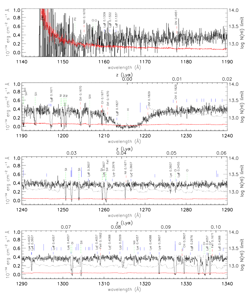
Figure 1: PKS 0405–123 data and $1\sigma$ errors (red) binned by 3 pixels for presentation only. Grey dash-triple dotted curve: 80% detection threshold in $\log N(\mbox{{H~{}I}})$ (right axis). Long, bold (red) ticks: Ly$\alpha$ lines with metals. Long/medium/short unlabelled (blue) ticks: Ly$\alpha$ forest ($z$ on upper axis) with $\log\mbox{$N_{HI}$}\geq 13.3$, $13.1\leq\log\mbox{$N_{HI}$}<13.3$ in the weak survey (§ 2), other Ly$\alpha$ lines respectively. Higher order Lyman lines are labelled. Medium dashed (red) ticks: intervening metal lines. Medium dotted (green) ticks: Galactic metal absorption.

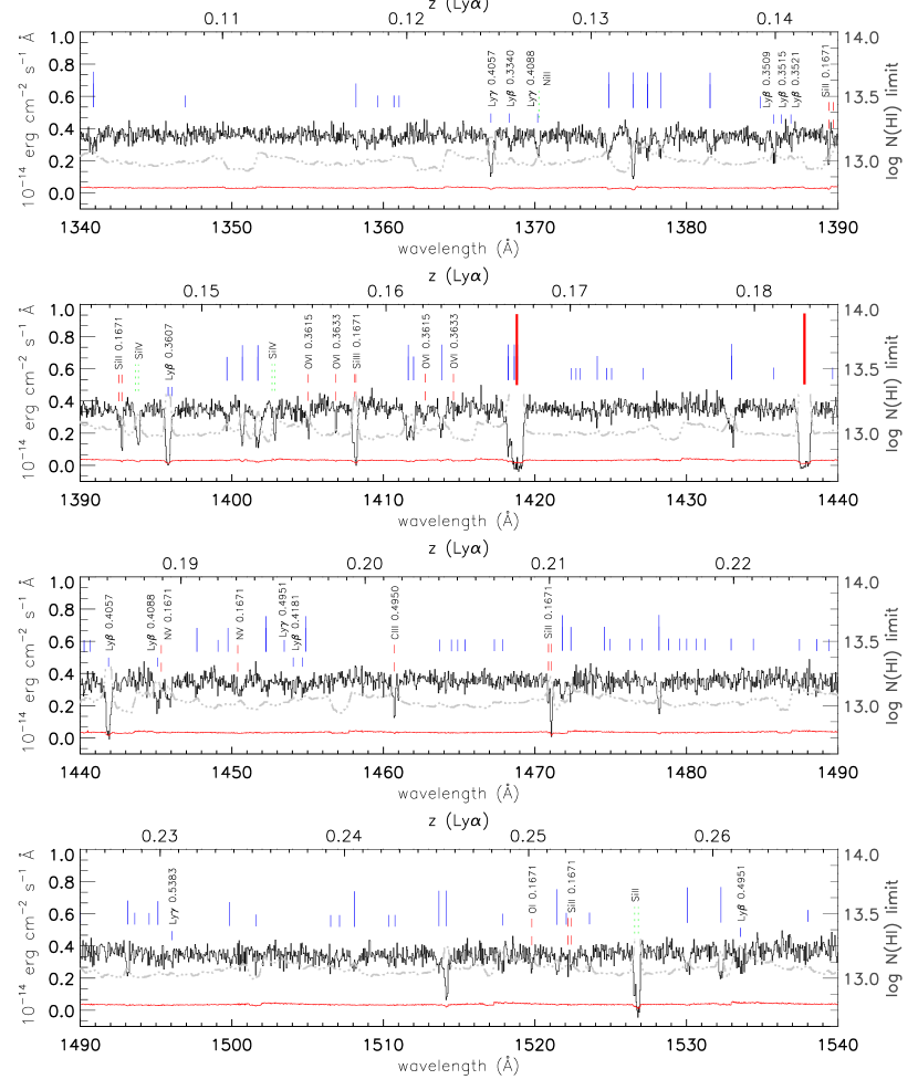
Figure 1: Continued.

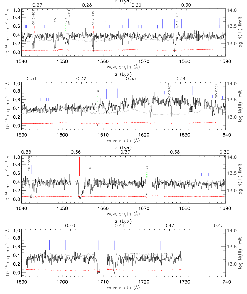
Figure 1: Continued.

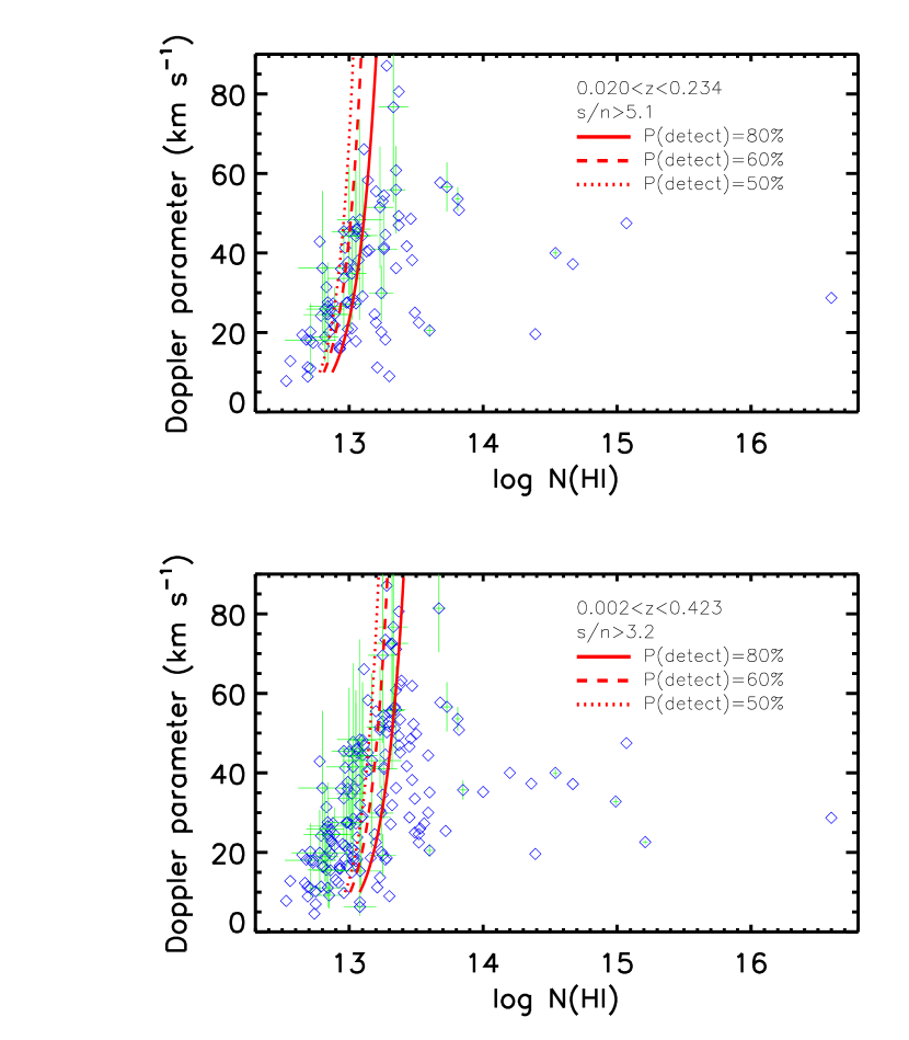
Figure 2: H I column densities and Doppler parameters. Top: Ly$\alpha$ forest sample over $0.020<z<0.234$, which is the redshift range used for our sample of $\log\mbox{$N_{HI}$}\geq 13.1$ (s/n ratio $>5.1$ per pixel, $b=40$ km s^-1). Open diamonds: data points. For clarity, only error bars for every third point are shown. Solid, dashed and dotted lines indicate the boundaries of the 80%, 60% and 50% detection probabilities from simulations in § 4. Below: As above, but for the Ly$\alpha$ forest sample over $0.002<z<0.423$, which is used for our sample of $\log\mbox{$N_{HI}$}\geq 13.3$ (s/n ratio $>3.2$ per pixel, $b=40$ km s^-1).

Figure 3: Comparison of H I column densities and Doppler parameters. Left: H I column densities for the fits done by Carswell and Williger. Right: Doppler parameters. Only systems in the strong and weak samples, and for which similar sets of Lyman series lines were fitted, are shown.

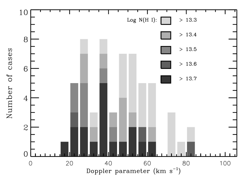
Figure 4: Ly$\alpha$ Doppler parameter distribution for a series of minimum $\log\mbox{$N_{HI}$}$ thresholds. The tail at high values is likely a result of unresolved blends.

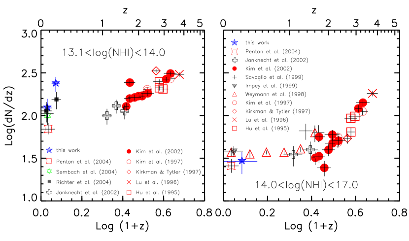
Figure 5: Left: Ly$\alpha$ forest redshift density $dN/dz$ for $13.1<\log\mbox{$N_{HI}$}<14.0$. The high and low redshift stars correspond to high and low redshift halves of our sample, respectively, and show clear evidence of cosmic variance. Right: $14.0<\log\mbox{$N_{HI}$}<17.0$ (right). Error bars show redshift bins and Poissonian errors in $dN/dz$.

Figure 6: Redshift density for Ly$\alpha$ absorbers with $13.1\leq\log\mbox{$N_{HI}$}<14.0$ where the detection probability for a system with $\log\mbox{$N_{HI}$}=13.1$ is 80% . Errors are based on Poisson statistics. Dotted line: expected value for uniform distribution in $z$.

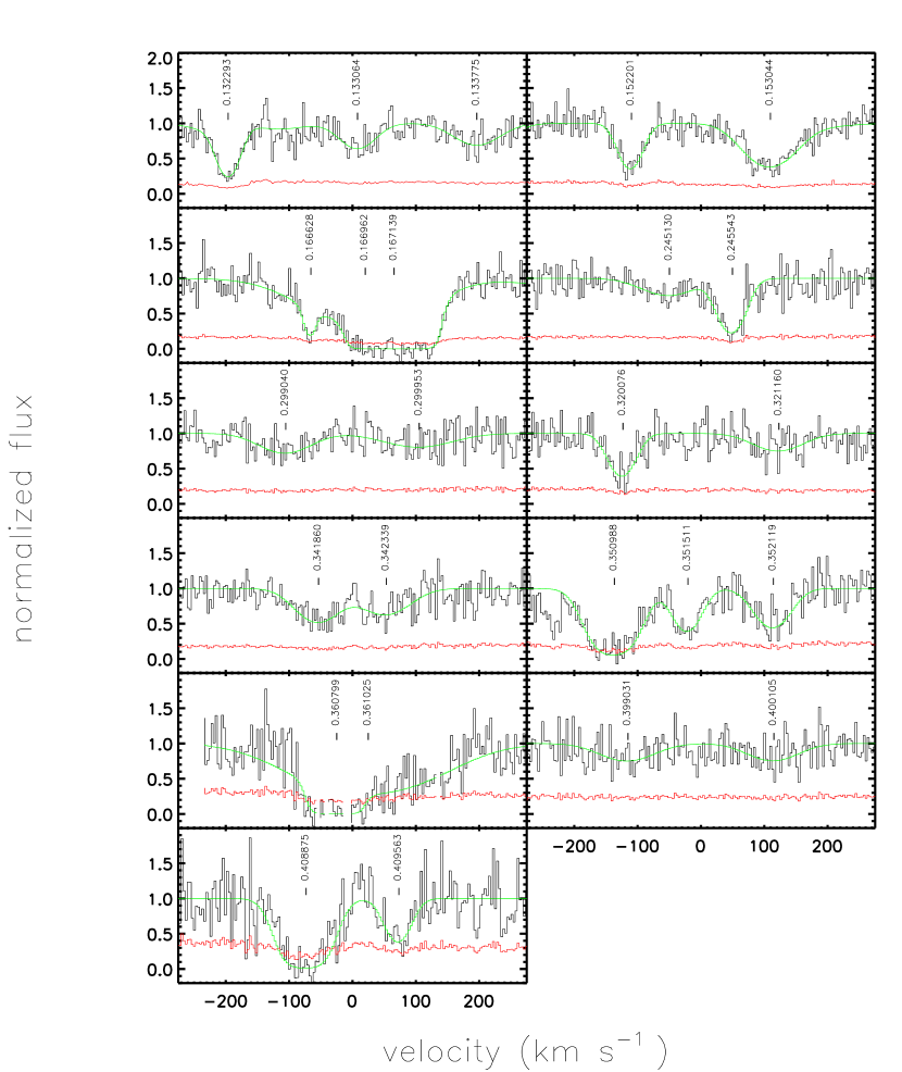
Figure 7: Ly$\alpha$ pairs with velocity separation $\Delta v<250$ km s^-1 for the strong sample. The data, $1\sigma$ error array and Voigt profile fit are shown. Ly$\alpha$ lines are marked by ticks and redshifts. For clarity, noise spikes have been suppressed.

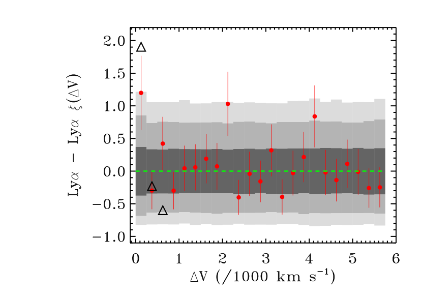
Figure 8: Two point correlation function for the strong Ly$\alpha$ sample ($\log\mbox{$N_{HI}$}\geq 13.3$), which is the column density threshold with the most significant signal. Shaded regions denote 68, 95, 99% confidence limits from 10⁴ Monte Carlo simulations. The value at $\Delta v<250$ km s^-1 has a probability of occurrence from unclustered data of $P=0.005$. Simulated line lists have been filtered to eliminate pairs with velocity splittings of $\Delta v<43$ km s^-1. Error bars show example $1\sigma$ Poissonian errors. The triangles show expected values from the simulations of Davé, Katz, & Weinberg (2003) for the same column density threshold; the simulation box artificially lowers the value of $\xi$ in the higher two velocity bins. The data differ from the simulation at $\Delta v<250$ km s^-1 at the 1.2 $\sigma$ level.

Figure 9: CFHT r-band image centered on PKS 0405–123. The field size is 9 arcmin (2.9 local frame Mpc at $z=0.4$), and north and east are indicated by the compass. Galaxies correspond to numbers in Table The Low-Redshift Ly$\alpha$ Forest toward PKS 0405–123^1,2. PKS 0405–123 is designated by Q.

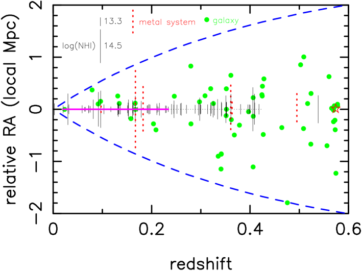
Figure 10: Ly$\alpha$ absorbers and galaxies toward PKS 0405–123, projected onto the declination plane. Vertical lines: Ly$\alpha$ systems, with length proportional to $\log\mbox{$N_{HI}$}$. Dashed lines and arrows: metal absorbers. Dots: galaxies. Thick line at RA=0: $z$ limits where survey is complete to $\log\mbox{$N_{HI}$}=13.1$; only absorbers corresponding to the local 80% detection probability threshold are shown. Thin line at RA=0: $z$ limits where survey is complete to $\log\mbox{$N_{HI}$}=13.3$. Star: PKS 0405–123. Dashed cone: scope corresponding to a 5 arcmin radius.

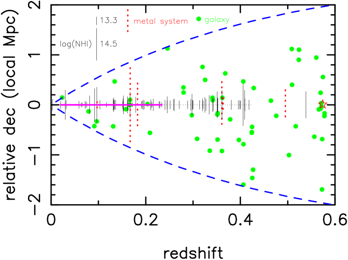
Figure 11: As Fig. 10, but projected onto the right ascension plane.

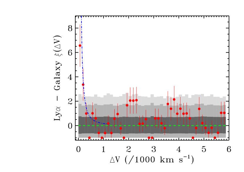
Figure 12: Two point correlation function in velocity space for the Ly$\alpha$ forest and galaxies within 2 Mpc projected distance, with $\log\mbox{$N_{HI}$}\geq 13.5$, the threshold at which the correlation significance is maximum. Shaded regions: 68, 95, 99% confidence limits from $10^{4}$ Monte Carlo simulations. Dash-dotted line: Galaxy-galaxy correlation function from Table 1 of Zehavi et al. (2004), weighted by the number of galaxies, interpolated for $M_{r}=-20$ and set to $z=0.2$. Error bars show example $1\sigma$ Poissonian errors.

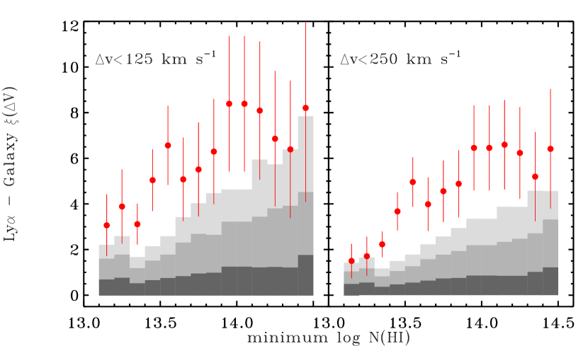
Figure 13: Two point correlation function in velocity space for the Ly$\alpha$ forest and galaxies within 2 Mpc projected distance, as a function of minimum absorber H I column density threshold, for $\Delta v<125$ km s^-1 (left panel) and $\Delta v<250$ km s^-1 (right panel). Symbols and shading are as in Figure 12. There is a marginal effect that the weakest absorbers have their strongest signal at $\Delta v<125$ km s^-1, while the strongest ones strengthen the significance of their signal out to $\Delta v<250$ km s^-1. Such behavior would be consistent with higher column density systems having a longer correlation length with galaxies, which would be expected from larger density perturbations.

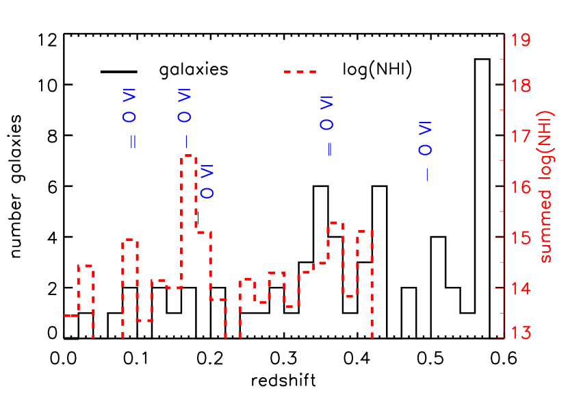
Figure 14: Galaxy counts (solid lines, left axis) and summed Ly$\alpha$ forest H I column density (dashed lines, right axis) counting $\log\mbox{$N_{HI}$}\geq 13.3$ at $0.002<z<0.423$, as a function of redshift toward PKS 0405–123. Redshifts of O VI absorbers are indicated with ticks. Although the galaxy counts are incomplete, and the STIS Ly$\alpha$ forest data are limited to $z<0.42$, there is a striking correlation between the local galaxy density and local H I column density in the Ly$\alpha$ forest. The Spearman rank coefficient for this binning is $\rho=0.67$ with a two-tailed probability of $p_{\rho}=0.001$. The Kendall rank coefficient is $\tau=0.56$ with a corresponding two-tailed probability of $p_{\tau}=0.0004$.

References

- Adelberger et al. (2003) Adelberger, K. L., Steidel, C. C., Shapley, A. E., Pettini, M. 2003, ApJ, 584, 45
- Berlind et al. (2003) Berlind, A. A., Blanton, M. R., Hogg, D. W., Weinberg, D. H., Davé, R., Eisenstein, D. J., Katz, N. 2003, ApJ, submitted, astro-ph/0406633
- Bouché, Murphy & Peroux (2004) Bouché, N., Murphy, M. T. & Péroux, C. 2004, MNRAS, 354, L25
- Bowen et al. (1995) Bowen, D. V., Blades, J. C., & Pettini, M. 1995, ApJ, 448, 634
- Bowen et al. (2002) Bowen, D. V., Pettini, M., Blades, J. C. 2002, ApJ, 580, 169
- Carswell, Schaye, & Kim (2002) Carswell, R. F., Schaye, J., & Kim, T.-S. 2002, ApJ, 578, 43
- Chen et al. (2001) Chen, H.-W., Lanzetta, K. M., Webb, J. K., Barcons, X. 2001, ApJ, 559, 654
- Chen & Prochaska (2000) Chen, H.-W. & Prochaska, J. X. 2000, ApJ, 543, 9
- Chen et al. (2005) Chen, H.-W. & Prochaska, J. X., Weiner, B. J., Mulchaey, J. S., Williger, G. M. 2005, ApJ, 629, L25, astro-ph/0507621
- Cowie et al. (1995) Cowie, L. L., Songaila, A., Kim, T.-S., & Hu, E. M. 1995, AJ, 109, 1522
- Cristiani et al. (1995) Cristiani, S., D’Odorico, S., Fontana, A., Giallongo, E., Savaglio, S. 1995, MNRAS, 273, 1016
- Crotts (1987) Crotts, A. P. S. 1987, MNRAS, 228, 41P
- Davé (1997) Davé, R. 1997, in Proc. IAGUSP Workshop, “Young Galaxies and QSO Absorbers”, eds. S. Viegas, R. Gruenwald, R. de Carvalho (San Francisco: ASP Conference Series v.114), p.67, astro-ph/9609060
- Davé et al. (1998) Davé, R., Hellsten, U., Hernquist, L., Katz, N., Weinberg, D. H. 1998, ApJ, 509, 661
- Davé et al. (2001) Davé, R. et al. 2001, ApJ, 552, 473
- Davé et al. (1999) Davé, R., Hernquist, L., Katz, N., Weinberg, D. H. 1999, ApJ, 511, 521