Pulsar timing and the detection of black hole binary systems in globular clusters

Abstract

The possible existence of intermediate mass binary black holes (IMBBHs) in globular clusters (GCs) offers a unique geometry in which to detect space-time oscillations. For certain pulsar-IMBBH configurations possible within a GC, the usual far-field plane wave approximation for the IMBBH metric perturbation severely underestimates the magnitude of the induced pulsar pulse time-of-arrival (TOA) fluctuations. In this letter, the expected TOA fluctuations induced by an IMBBH lying close to the line-of-sight between a pulsar and the Earth are calculated for the first time. For an IMBBH consisting of $10M_{\odot}$ and $10^{3}M_{\odot}$ components, a 10 year orbital period, and located 0.1 lyr from the Earth-Pulsar line of sight, the induced pulsar timing residual amplitude will be of order 5 to 500 ns.

1. Introduction

The unique stability of the electromagnetic pulses emitted by radio pulsars could allow one to detect the presence of gravitational wave radiation. It is normally assumed that the pulsar, Earth, and all points along the line-of-sight between the pulsar and the Earth are located far enough away from the source that the space-time oscillations may be treated as gravitational plane waves (Sazhin, 1978; Detweiler, 1979). Recently, it has been suggested that intermediate mass black hole binary systems may form in the centers of Globular Clusters (GCs) (Miller, 2002; Will, 2004; Miller & Colbert, 2004). Given the high density of radio pulsars in GCs together with the relatively small scale length (100 pc) of a GC, it is possible to find a pulsar whose line-of-sight will pass closer to the binary system than its end points. It is even possible that the pulsar itself may lie close to the binary system. It is shown in this letter that this scenario differs from the plane gravitational wave case in two important ways. First, the amplitude of the induced residuals depends on the distance of closest approach, or impact parameter, between the binary system and the Earth-pulsar line-of-sight. Second, since the closest distance may be well within one gravitational wavelength, the near-field terms will play the dominant role in inducing the observed pulsar pulse arrival time fluctuations.

In this letter, the effect of the gravitational field of a binary system on pulsar timing residuals are calculated. This is the first time both near and far field terms are included in this calculation and no assumptions are made about the structure of the emitted gravitational wave front. The results are accurate to order $(v/c)^{2}$ and $(d/r)^{2}$ where $v$ is the characteristic relative velocity of the mass-energy within the source, $c$ is the speed of light, $d$ is the length scale of the binary system, and $r$ is the smallest distance between the binary system and the Earth-pulsar line of sight. The general expressions for the timing residuals derived here may be applied to pulsar timing data to constrain the properties of putative black hole binary systems.

It should be noted that the 20 new millisecond pulsars recently discovered in the dense globular cluster Terzan 5 (Ransom et al., 2005) may provide an interesting application of these results. The large number of pulsars together with this cluster’s high central density ($\approx 10^{6}L_{\odot}/\mathrm{pc}^{3}$) make it a good candidate to detect or at least limit the existence of an intermediate mass binary black hole (IMBBH) system in its core.

In the next section, the general effect of a binary system on the arrival times of pulses emitted by a pulsar is calculated. We make use of geometric units where $G=c=1$. Order of magnitude estimates of the induced timing residuals are also made for astrophysically relevant systems. The results are summarized in the last section.

2. Calculating the Residuals

The curvature of space-time will cause the observed pulsar frequency to vary as a function of time. The timing residuals, $R(t)$, are given by(Detweiler, 1979)

$$R(t)=\int_{0}^{t}\frac{\nu_{o}-\nu_{e}}{\nu_{e}}dt\;,$$ (1)

where $t$ is time, $\nu_{o}$ is the observed frequency, and $\nu_{e}$ is the emitted frequency. The frequency shifts will be calculated using perturbative methods. Given the four velocity of an observer, $V^{\mu}$, the observed pulse frequency is given by $\nu=-V^{\mu}K_{\mu}$ where $K_{\nu}$ is the dual to the photon four velocity. Let $V^{\mu}=\bar{V}^{\mu}+\delta V^{\mu}$ and $K_{\mu}=\bar{K}_{\mu}+\delta K_{\mu}$, where the barred quantities are the unperturbed values, and $\delta V$ and $\delta K$ are the corresponding perturbations. For the purposes of this discussion, we choose the unperturbed four-velocities of both the emitter and the observer to be 1 in the time direction and zero for the three spatial components. To lowest order, the timing residuals are given by

$$R(t)=\int_{0}^{t}\frac{\delta K_{0}^{o}-\delta K_{0}^{e}+(\delta V^{o\mu}-\delta V^{e\mu})\bar{K}_{\mu}}{\bar{K}_{0}}dt\;.$$ (2)

The last term on the right hand side is the standard Doppler shift due to the relative velocity between the source and the emitter. The first two terms are determined by the actual path of the photons as they travel towards the receiver.

The geodesic equations will be used to solve for both $\delta K$ and $\delta V$. To lowest order, these equations take the following form:

$$\frac{d\delta K_{\alpha}}{d\lambda}-\frac{1}{2}g_{\mu\nu,\alpha}\bar{K}^{\mu}\bar{K}^{\nu} = 0\;,$$ (3)

$$\frac{d\delta V_{\alpha}}{d\tau}-\frac{1}{2}g_{\mu\nu,\alpha}\bar{V}^{\mu}\bar{V}^{\nu} = 0\;,$$ (4)

where $\lambda$ is the affine parameter along the light-ray path, $\tau$ is the proper time of the observer, and $g_{\mu\nu}$ is the space-time metric. The metric is assumed to be of the form $\eta_{\mu\nu}+h_{\mu\nu}$ where $\eta_{\mu\nu}$ is the flat Minkowsky metric and $h_{\mu\nu}$ is a small perturbation given, at space-time location $(t,\vec{r})$, by:

$$h_{\mu\nu}(t,\vec{r})=\int\frac{\bar{T}_{\mu\nu}(t-|\vec{r}-\vec{r}^{\prime}|,\vec{r}^{\prime})}{|\vec{r}-\vec{r}^{\prime}|}d^{3}\vec{r}^{\prime}\;,$$ (5)

where $\bar{T}_{\mu\nu}$ is the trace-reversed stress energy tensor of the region generating the space-time perturbation.

The timing residual due to ray path propagation will be calculated to first order in $h$ using Eq. (3) rewritten in integral form as:

$$\frac{\delta K^{o}_{0}-\delta K^{e}_{0}}{\bar{K}_{0}} = \int_{z_{e}}^{z_{o}}H(t+z,b\hat{y}+z\hat{z})dz$$ (6)

$$H(t,\vec{r}) = \frac{1}{2}(h_{00,0}+h_{zz,0}+2h_{0z,0}),$$ (7)

given in the black hole barycentered coordinate system shown in Fig. 1, with $\hat{z}$ pointing parallel to the light ray from the radio emitter to the observer (so that $z=\bar{K}^{0}\lambda$), and $\hat{x}$ pointing from the black hole binary barycenter to the closest point on that ray. The emitter and observer positions $z_{e}$ and $z_{o}$, and the impact parameter $b$, are defined in Fig. 1.

Using Eq. (5), $h_{\mu\nu}$ can be calculated using standard perturbative techniques to order $(v/c)^{2}$ and $(d/r)^{2}$ where $v$ is the characteristic velocity of the source elements relative to their center of mass, and $d$ is the characteristic size scale of the source. Remarkably, $H$ can be written to this order as $H=dF/dz$, where $F$ is given by:

$$F(t,\vec{r}) = \frac{\dot{Q}_{rr}-\dot{Q}_{i}^{i}}{(r-z)r}+\frac{\dot{Q}_{rr}+\dot{Q}_{zz}-2\dot{Q}_{rz}}{(r-z)^{2}}+$$ (8)

$$\frac{\ddot{Q}_{rr}+\ddot{Q}_{zz}-2\ddot{Q}_{rz}}{r-z}.$$

$Q_{ij}$ is the second moment of the mass-energy distribution defined as

$$Q_{ij}=\int T^{00}r_{i}^{\prime}r_{j}^{\prime}d^{3}\vec{r}^{\prime},$$ (9)

and the “$\dot{}$” represents the time derivative. Given that the mass-energy distribution is usually specified in the ($\hat{x},\hat{y},\hat{z}$) coordinate system, it is useful to note that $Q_{rr}=Q_{zz}\cos^{2}\theta+2Q_{zx}\cos\theta\sin\theta+Q_{xx}\sin^{2}\theta$, $Q_{rz}=Q_{zz}\cos\theta+Q_{zx}\sin\theta$, and $Q_{i}^{i}=Q_{xx}+Q_{yy}+Q_{zz}$, where $r=\sqrt{z^{2}+b^{2}}$ and $\theta=\arccos{z/r}$.

Next, the contribution due to the 4-velocity of the observer and emitter will be calculated. Eq. (4) determines the acceleration of the body in question. Under the assumption that the body does not move appreciably under the influence of the metric perturbation so that the time derivatives of $r$ may be ignored,

$$\frac{\delta V^{\mu}\bar{K}_{\mu}}{\bar{K}_{0}}=G(t,\vec{r})-G(0,\vec{r})$$ (10)

where

$$G(t,\vec{r}) = \frac{2\ddot{Q}_{rz}-\left(1+\frac{z}{r}\right)\frac{\ddot{Q}_{rr}}{2}-\left(1+\frac{z}{r}\right)\frac{\ddot{Q}_{i}^{i}}{2}}{r}+$$ (11)

$$\frac{3\dot{Q}_{rz}-3\dot{Q}_{rr}\left(1+\frac{z}{r}\right)-\frac{\dot{Q}_{i}^{i}}{2}}{r^{2}}+$$

$$\frac{3Q_{rz}-\frac{3}{2}\left(1+\frac{5z}{r}\right)Q_{rr}+\left(1+\frac{3z}{r}\right)\frac{Q_{i}^{i}}{2}}{r^{3}}+$$

$$\int_{0}^{t}\left(\frac{3Q_{rz}+\frac{3z}{2r}Q_{i}^{i}-\frac{15z}{2r}Q_{rr}}{r^{4}}\right)dt^{\prime}$$

Using Eqs. (2), (6), and (10), the complete residual may be written as

$$R(t) =\int_{0}^{t} \{F(t^{\prime},\vec{r}_{o})-F(t_{\mathrm{ret}},\vec{r}_{e})+$$ (12)

$$G(t^{\prime},\vec{r}_{o})-G(t_{\mathrm{ret}},\vec{r_{e}})\}\,dt^{\prime}$$

where $t_{\mathrm{ret}}=t^{\prime}-[z_{o}-z_{e}]$. Note that the terms which will ultimately give rise to secular terms (i.e. $G(0,\vec{r})$) are not included in the above expression.

The above derivation assumes that the pulsar and observer are stationary in the barycentric frame of the binary system. However, for relative velocities $\ll c$, Eqs. 8, 11, and 12 give the correct leading-order behavior of the residual, provided we allow $z$ and $r$ to be functions of $t$.

For the case when $z_{e}$ goes to negative infinity and $z_{o}$ goes to positive infinity, one can show that the expected residual does not go to zero. Instead it limits to:

$$R(t)=2\int_{0}^{t}\frac{\dot{Q}_{xx}(t^{\prime}-r_{o})-\dot{Q}_{yy}(t^{\prime}-r_{o})}{b(t^{\prime})^{2}}\;dt^{\prime}$$ (13)

Now when the source of the gravitational perturbation is a massive binary system, we can give an explicit form for the quadrapole moment in the barycentric frame:

$$Q_{ij}=\mu s_{i}s_{j}\;,$$ (14)

where $\mbox{\boldmath$s$\unboldmath}=\mbox{\boldmath$s$\unboldmath}_{2}-\mbox{\boldmath$s$\unboldmath}_{1}$ is the separation vector and $\mu=m_{1}m_{2}/(m_{1}+m_{2})$ is the reduced mass of the binary system with component masses $m_{1}$ and $m_{2}$. Using standard astrometric notation, we can write this directly in terms of the inclination $i$ of the orbit to the plane of the sky, the position angle $\Omega$ of the ascending node, the argument of periapse $\omega$, and the true anomaly $\upsilon$ as shown in Fig. 2. There $\hat{r}_{o}$ points towards the observer, $\hat{\delta}$ points towards the North celestial pole, $\hat{s}_{p}$ is the direction of the separation vector at periapse, $\hat{L}$ points along the orbital angular momentum axis, and $\hat{u}$ points towards the ascending node of the orbit. Defining a second unit vector $\hat{w}=\hat{L}\times\hat{u}$ in the plane of the orbit, we can write the motion of the binary in that coordinate system as:

$$\mbox{\boldmath$s$\unboldmath}=\textstyle a\frac{1-e^{2}}{1+e\cos\upsilon}\{\cos(\omega+\upsilon)\hat{u}+\sin(\omega+\upsilon)\hat{w}\}$$ (15)

where $a$ is the orbital semi-major axis and $e$ is the eccentricity. Noting that $\hat{x}^{\prime}=\hat{x}\cos\theta_{o}-\hat{z}\sin\theta_{o}$ is the projection of $\hat{x}$ into the plane of the sky, and defining its position angle $B$ in the same sense as $\Omega$, the separation vector in the $(\hat{x},\hat{y},\hat{z})$ coordinate system is:

$$s = \hat{x}[\;\;\,s_{u}\cos(\Omega-B)\cos\theta_{o}-s_{w}\sin(\Omega-B)\cos\theta_{o}\cos i+s_{w}\sin\theta_{o}\sin i]$$ (16)

$$+ \hat{y}[\;\;\,s_{u}\sin(\Omega-B)+s_{w}\cos(\Omega-B)\cos i]$$

$$+ \hat{z}[-s_{u}\cos(\Omega-B)\sin\theta_{o}+s_{w}\sin(\Omega-B)\sin\theta_{o}\cos i+s_{w}\cos\theta_{o}\sin i]\;.$$

Here we have taken $\upsilon$ to be our independent parameter, which must be evaluated at appropriate retarded times. The time derivatives can be computed analytically using Kepler’s law $\dot{\upsilon}=(2\pi/P)(1+e\cos\upsilon)^{2}/(1-e^{2})^{3/2}$, where $P=2\pi\sqrt{a^{3}/M_{t}}$ is the orbital period and $M_{t}=m_{1}+m_{2}$ the total mass of the system. Many standard techniques exist for computing the full time dependence of $\upsilon(t)$, one of the more generic being to solve numerically the transcendental equation for the eccentric anomaly $E$:

$$\textstyle t-t_{p}=\frac{2\pi}{P}\left(E-e\sin E\right)\;,$$ (17)

where $t_{p}$ is a time of periapse passage, and then to compute $\upsilon$ via:

$$\textstyle\tan\left(\frac{\upsilon}{2}\right)=\sqrt{\frac{1+e}{1-e}}\tan\left(\frac{E}{2}\right)\;.$$ (18)

For simplicity, though, we will continue to write the expressions in terms of (retarded) $\upsilon$.

Solving explicitly for the case where $b\ll r_{e},r_{o}$ and $b$ is effectively constant over the time of observation, Eq. (13) becomes:

$$R(t) = \textstyle 2\frac{\mu a^{2}}{b^{2}}\left(\frac{1-e^{2}}{1+e\cos\upsilon}\right)^{2}\Big{[}\sin 2(\omega+\upsilon)\sin 2(\Omega-B)\cos i+$$ (19)

$$\{\sin^{2}(\omega+\upsilon)\cos^{2}i-\cos^{2}(\omega+\upsilon)\}\cos 2(\Omega-B)\Big{]}\;.$$

Next, order of magnitude estimates are made for the amplitude of the induced residuals using the above results. Two cases will be considered. In case I, both the pulsar and the observer are infinitely far away from the gravitational wave source but the impact parameter is finite. In case II, the observer is infinitely far away, but the pulsar is at $|z_{e}|\sim b\ll P$ (i.e. the pulsar is in the near zone of the gravitational field).

In case I, the amplitude of the induced residuals can be estimated using Eq. (19): $R_{I}\sim 2\mu a^{2}/b^{2}=2\mu M_{t}^{2/3}(P/2\pi)^{4/3}/b^{2}$. For the nominal case of a binary system with $10M_{\odot}$ and $10^{3}M_{\odot}$ components, a 10 year orbital period, and an impact parameter of 0.1 lyr, one obtains the following order of magnitude estimates:

$$R_{I} \sim 5\mbox{ns}\left(\frac{\mu}{10M_{\odot}}\right)\left(\frac{M_{t}}{10^{3}M_{\odot}}\right)^{2/3}\left(\frac{b}{.1~{}\mbox{lyr}}\right)^{-2}\left(\frac{P}{10~{}\mbox{yr}}\right)^{4/3}$$ (20)

In case II, the residuals induced by the motion of the binary system will be dominated by the last term in Eq. (11). Hence an estimate for the residual amplitude is given by $R_{II}\sim(3/4)\mu M_{t}^{2/3}(P/2\pi)^{10/3}/b^{4}$. For the same system discussed above, one obtains the following:

$$R_{II} \sim 500\mathrm{ns}\left(\frac{\mu}{10M_{\odot}}\right)\left(\frac{M_{t}}{10^{3}M_{\odot}}\right)^{2/3}\left(\frac{b}{.1~{}\mbox{lyr}}\right)^{-4}\left(\frac{P}{10~{}\mbox{yr}}\right)^{10/3}$$ (21)

In order to understand the above scaling, note that the impact parameter, $b$, is the only external scale factor in the problem and that the residuals are proportional to the quadrapole moment $Q\sim\mu a^{2}$. A simple dimensional argument therefore gives $R$ scaling as $\mu a^{2}/b^{2}$, times $P/b$ for every time integral of $Q$ in the leading-order term. Case I involves no time integrals while Case II has two. Kepler’s law is then used to write $a$ in terms of the orbital period.

3. Application and Discussion

General expressions for the periodic timing residuals induced by a binary system were calculated. It was shown that systematic variations in the pulsar timing residuals depend not only on the location of the pulsar and the observer, but also on how close the binary system is to the pulsar observer line-of-sight. As long as the line-of-sight impact parameter is finite, a non-zero residual amplitude can still occur even if both the pulsar and the observer are infinitely far away from the binary system. For a given impact parameter, the residuals calculated using case I and case II represent the range of possible residual amplitudes provided that $z_{e}\lesssim 0$. In other words, the pulsar must be near or behind the binary system.

Globular clusters present an interesting opportunity to discover intermediate mass binary black holes using pulsar timing. Table 1 shows the timing residuals, for cases I and II, that a $10M_{\odot}+10^{3}M_{\odot}$ binary system with a 10 year period would induce on known pulsars near (as specified by the impact parameter $b$) to the cores of their respective clusters. All pulsars in the table have periods $<10$ ms. By way of comparison, the root-mean-square (RMS) timing noise for millisecond pulsars is approaching the level of 100ns or better (van Straten et al., 2001). New efforts like the Parkes Pulsar Timing Array (PPTA) project are actively working to improve the RMS noise level. The proposed square kilometer array (SKA) project will provide timing precisions as low as 10 ns in the next 10–20 years and will also uncover all pulsars beamed at Earth within globular clusters(Cordes et al., 2004; Kramer et al., 2004).

Of course, a single pulsar could never definitely detect a binary system, although it could be suggestive. In order to make a strong case, timing residual oscillations must be seen in two or more pulsars and these oscillation must be consistent with the same binary system. The 20 millisecond pulsars in Terzan 5 may offer such an opportunity(Ransom et al., 2005).

Part of this research was carried out at the Jet Propulsion Laboratory, California Institute of Technology, under a contract with the National Aeronautics and Space Administration and funded through the internal Research and Technology Development program.

Figure 1.— System configuration and coordinate system.

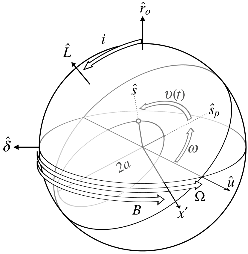
Figure 2.— Binary orbital parameters.

Table 1Residuals induced in globular cluster pulsars by a $10M_{\odot}+10^{3}M_{\odot}$, 10-year binary

Globular Cluster	Pulsar	$b$ (lyr)	RI (ns)	RII (ns)	Reference
47 Tuc	J0024-7204O	0.26	0.8	11	Freire et al. (2003)
47 Tuc	J0024-7204W	0.34	0.5	4	Camilo et al. (2000)
NGC 6266	J1701-3006B	0.18	1.6	50	Possenti et al. (2003)
NGC 6624	B1820-30A	0.37	0.4	3	Biggs et al. (1994)
M28 (NGC 6626)	B1821-24	0.12	4	200	Rutledge et al. (2004)
NGC 6752	J1910-5959B	0.38	0.4	2	D’Amico et al. (2002)
NGC 6752	J1910-5959E	0.49	0.2	0.9	D’Amico et al. (2002)
M15 (NGC 7078)	B2127+11D	0.19	1.4	40	Anderson (1993)
M15 (NGC 7078)	B2127+11H	0.37	0.4	3	Anderson (1993)

References

- Anderson (1993) Anderson, S. B. 1993, Ph.D. Thesis
- Biggs et al. (1994) Biggs, J. D., Bailes, M., Lyne, A. G., Goss, W. M., Fruchter, A. S., & Biggs, J. D. 1994, MNRAS, 267, 125
- Camilo et al. (2000) Camilo, F., Lorimer, D. R., Freire, P., Lyne, A. G., & Manchester, R. N. 2000, ApJ, 535, 975
- Cordes et al. (2004) Cordes, J. M., Kramer, M., Lazio, T. J. W., Stappers, B. W., Backer, D. C., & Johnston, S. 2004, New Astronomy Review, 48, 1413
- D’Amico et al. (2002) D’Amico, N., Possenti, A., Fici, L., Manchester, R. N., Lyne, A. G., Camilo, F., & Sarkissian, J. 2002, ApJ, 570, L89
- Detweiler (1979) Detweiler, S. 1979, ApJ, 234, 1100
- Freire et al. (2003) Freire, P. C., Camilo, F., Kramer, M., Lorimer, D. R., Lyne, A. G., Manchester, R. N., & D’Amico, N. 2003, MNRAS, 340, 1359
- Freire et al. (2001) Freire, P. C., Camilo, F., Lorimer, D. R., Lyne, A. G., Manchester, R. N., & D’Amico, N. 2001, MNRAS, 326, 901
- Kramer et al. (2004) Kramer, M., Backer, D. C., Cordes, J. M., Lazio, T. J. W., Stappers, B. W., & Johnston, S. 2004, New Astronomy Review, 48, 993
- Lommen & Backer (2001) Lommen, A. N., & Backer, D. C. 2001, ApJ, 562, 297
- Miller (2002) Miller, M. C. 2002, ApJ, 581, 438
- Miller & Colbert (2004) Miller, M. C., & Colbert, E. J. M. 2004, International Journal of Modern Physics D, 13, 1
- Possenti et al. (2003) Possenti, A., D’Amico, N., Manchester, R. N., Camilo, F., Lyne, A. G., Sarkissian, J., & Corongiu, A. 2003, ApJ, 599, 475
- Ransom et al. (2005) Ransom, S. M., Hessels, J. W. T., Stairs, I. H., Freire, P. C. C., Camilo, F., Kaspi, V. M., & Kaplan, D. L. 2005, Science, 307, 892
- Rutledge et al. (2004) Rutledge, R. E., Fox, D. W., Kulkarni, S. R., Jacoby, B. A., Cognard, I., Backer, D. C., & Murray, S. S. 2004, ApJ, 613, 522
- Sazhin (1978) Sazhin, M. V. 1978, Sov. Astron., 22, 36
- van Straten et al. (2001) van Straten, W., Bailes, M., Britton, M., Kulkarni, S. R., Anderson, S. B., Manchester, R. N., & Sarkissian, J. 2001, Nature, 412, 158
- Will (2004) Will, C. M. 2004, ApJ, 611, 1080