Cosmological parameters from combined second- and third-order aperture mass statistics of cosmic shear

We present predictions for cosmological parameter constraints from combined measurements of second- and third-order statistics of cosmic shear. We define the generalized third-order aperture mass statistics $\langle M_{\rm ap}^{3}\rangle$ and show that it contains much more information about the bispectrum of the projected matter density than the skewness of the aperture mass. From theoretical models as well as from $\Lambda$CDM ray-tracing simulations, we calculate $\langle M_{\rm ap}^{2}\rangle$ and $\langle M_{\rm ap}^{3}\rangle$ and their dependence on cosmological parameters. The covariances including shot noise and cosmic variance of $M_{\rm ap}^{2}$, $M_{\rm ap}^{3}$ and their cross-correlation are calculated using ray-tracing simulations. We perform an extensive Fisher matrix analysis, and for various combinations of cosmological parameters, we predict 1-$\sigma$-errors corresponding to measurements from a deep 29 square degree cosmic shear survey. Although the parameter degeneracies can not be lifted completely, the (linear) combination of second- and third-order aperture mass statistics reduces the errors significantly. The strong degeneracy between $\Omega_{\rm m}$ and $\sigma_{8}$, present for all second-order cosmic shear measures, is diminished substantially, whereas less improvement is found for the near-degenerate pair consisting of the shape parameter $\Gamma$ and the spectral index $n_{\rm s}$. Uncertainties in the source galaxy redshift $z_{0}$ increase the errors of all other parameters.

1 Introduction

In recent years, weak gravitational lensing by the large-scale matter distribution in the Universe has become an important tool for cosmology. Cosmic shear surveys have yielded constraints on cosmological parameters without the need for modeling the relation between luminous and dark matter (bias). In particular, the power spectrum normalization $\sigma_{8}$ has been obtained with less than 10 % uncertainty (van Waerbeke et al. 2005).

On the one hand, the observed sky area and thus the number of faint background galaxies increased dramatically with the advent of wide-field imaging cameras mounted onto large telescopes. On the other hand, measurement errors have decreased with further understanding of systematics together with new image analysis methods. These two advances were crucial in the evolution of cosmic shear towards a high-precision cosmology tool.

Cosmic shear is sensitive to inhomogeneities in the projected matter distribution out to redshifts of order unity, depending on the depth of the survey. It probes scales where fluctuations have started to grow non-linearly due to gravitational instabilities. These non-linearities along with projection effects erase most of the primordial features such as baryon wiggles in the power spectrum. Thus, cosmological parameters cannot be determined uniquely using second-order statistics alone; there exist substantial near-degeneracies, e.g. between $\Omega_{\rm m}$ and $\sigma_{8}$.

Because these degeneracies manifest themselves in a different way for shear statistics of different order, they can be lifted by combining e.g. second- and third-order statistics. An example is the reduced skewness of the convergence or projected surface mass density $\kappa$, which has been shown to not, or only weakly, depend on $\sigma_{8}$ and thus to be able to break the near-degeneracy with $\Omega_{\rm m}$ (Bernardeau et al. 1997; van Waerbeke et al. 1999).

Although the convergence cannot be observed directly, Schneider et al. (1998) defined the so-called aperture mass statistics ${M_{\rm ap}}$, which is a local convolution of $\kappa$ with a compensated filter, and which can be measured directly from the ellipticities of the background galaxies.

The first significant non-zero third-order cosmic shear signal was found by Bernardeau et al. (2002), who measured an integral over the three-point correlation function (3PCF) of shear in the VIRMOS-DESCART survey. From the same data, aperture mass skewness was detected later by Pen et al. (2003), and an upper limit for $\Omega_{\Lambda}$ was derived. A ${M_{\rm ap}}$ skewness detection at the $2\sigma$-level was obtained from the CTIO survey by Jarvis et al. (2004) who also derived handy expressions for the ${M_{\rm ap}}$ skewness in terms of the 3PCF. Both detections of $\langle M_{\rm ap}^{3}\rangle$ were obtained by integrating over the measured 3PCF.

In this paper, we demonstrate the improvement of cosmological parameter determination from cosmic shear, using combined measurements of the second- and generalized third-order aperture mass statistics. This latter quantity was introduced by Schneider et al. (2004) as the third-order correlator of ${M_{\rm ap}}$ for three different aperture radii, $\langle M_{\rm ap}^{3}(\theta_{1},\theta_{2},\theta_{3})\rangle\equiv\langle{M_{\rm ap}}(\theta_{1}){M_{\rm ap}}(\theta_{2}){M_{\rm ap}}(\theta_{3})\rangle$. Unlike the skewness $\langle M_{\rm ap}^{3}(\theta,\theta,\theta)\rangle\equiv\langle{M_{\rm ap}}(\theta){M_{\rm ap}}(\theta){M_{\rm ap}}(\theta)\rangle$, which depends on only one filter scale $\theta$, the generalized third-order aperture mass statistics contains information about the convergence bispectrum in principle over the full Fourier-space.

The reasons of employing ${M_{\rm ap}}$ instead of the shear correlation functions are multiple:

• $M_{\rm ap}$ is a scalar quantity, therefore odd powers of it such as $M_{\rm ap}^{3}$ have non-trivial expectation values. In contrast, no scalar can be formed from tri-linear combinations of the eight components of the 3PCF of shear (Schneider & Lombardi 2003; Takada & Jain 2003; Zaldarriaga & Scoccimarro 2003).

• From the aperture mass statistics, we get a measure of the residual systematics by its ability to separate the E- from the B-mode (Crittenden et al. 2002; Schneider et al. 2002). This is true for both second- and third-order.

• The integral relations between $\langle M_{\rm ap}^{3}\rangle$ and the bispectrum are much easier and numerically faster to evaluate than for the 3PCF (Schneider et al. 2004). The reason is that $\langle M_{\rm ap}^{3}\rangle$ is a local measure of the bispectrum, whereas the integral kernel for the 3PCF is a highly oscillating function with infinite support.

This paper is organized as follows. In Sect. 2, we describe the theoretical models that are employed for the power and bispectrum. We give the definition of the second- and generalized third-order aperture mass statistics and their relation to the power and bispectrum in Sect. 3, followed by a short description of the ray-tracing simulations. Section 4 addresses the calculation of the covariance matrices of ${M_{\rm ap}^{2}}$, ${M_{\rm ap}^{3}}$ and their cross-correlation. Finally, in Sect. 5 we present our results on cosmological parameter constraints from a Fisher matrix analysis.

2 Models of the power- and bispectrum

Statistical weak gravitational lensing on large scales probes the projected density field of the matter in the Universe, also called convergence $\kappa$. All second-order statistics of the convergence can be expressed as functions of the two-point correlation function (2PCF) of $\kappa$ or its Fourier transform, the power spectrum $P_{\kappa}$. Analogously, third-order statistics are related to the 3PCF of $\kappa$; its Fourier transform is the bispectrum $B_{\kappa}$.

The 3-D dark matter power spectrum has been extensively modeled using numerical simulations. Halo model approaches as well as fitting formulae give very accurate descriptions of the quasi-linear and highly non-linear regime on intermediate and small scales (Peacock & Dodds 1996; Smith et al. 2003; Cooray & Sheth 2002). Throughout this work, we employ the fitting formula of Peacock & Dodds (1996), which was also used by Scoccimarro & Couchman (2001) for their modeling of the bispectrum.

On the other hand, the bispectrum of the cosmological dark matter distribution is less securely known. It is well established that the primordial density fluctuations were Gaussian (e.g. Spergel et al. 2003). In the limit of linear perturbations, they remain Gaussian – thus the power spectrum alone contains all information about the large-scale structure. However, gravitational clustering is a non-linear process and, in particular at small scales, the mass distribution evolves to become highly non-Gaussian.

The bispectrum $B_{\kappa}$ of the convergence is defined by the following equation:

$$\left\langle\hat{\kappa}(\@vec{\ell}_{1})\hat{\kappa}(\@vec{\ell}_{2})\hat{\kappa}(\@vec{\ell}_{3})\right\rangle=(2\pi)^{2}\delta_{\rm D}(\@vec{\ell}_{1}+\@vec{\ell}_{2}+\@vec{\ell}_{3})$$ (1)

$$\hskip 30.00005pt\times\left[B_{\kappa}(\@vec{\ell}_{1},\@vec{\ell}_{2})+B_{\kappa}(\@vec{\ell}_{2},\@vec{\ell}_{3})+B_{\kappa}(\@vec{\ell}_{3},\@vec{\ell}_{1})\right],$$

where $\hat{\kappa}$ is the Fourier transform of $\kappa$ and $\delta_{\rm D}$ is Dirac’s delta function.

We assume the field $\kappa$ to be statistically isotropic, thus its bispectrum only depends on the moduli $\ell_{1},\ell_{2}$ of the wave vectors and their enclosed angle $\varphi$, $B_{\kappa}(\@vec{\ell}_{1},\@vec{\ell}_{2})\equiv b_{\kappa}(\ell_{1},\ell_{2},\varphi)$. Because of parity symmetry, $b_{\kappa}$ is an even function of $\varphi$.

In this work, we employ hyper-extended perturbation theory (HEPT, Scoccimarro & Couchman 2001) for a $\Lambda$CDM Universe as a model for the bispectrum. The HEPT fitting formula fits the $N$-body simulations with an accuracy of $\begin{array}[]{c}<\\ \sim\end{array}$ 15 percent, which is sufficient for our purpose. In HEPT, we can write

$$b_{\kappa}(\ell_{1},\ell_{2},\varphi)=\sum_{m=0}^{2}F_{2}^{(m)}(\ell_{1},\ell_{2})\cos^{m}(\varphi)\,\bar{b}_{\kappa}^{(m)}(\ell_{1},\ell_{2}),$$ (2)

with $F_{2}^{(0)}=10/7$, $F_{2}^{(1)}=\ell_{1}/\ell_{2}+\ell_{2}/\ell_{1}$, $F_{2}^{(2)}=4/7$. The functions $\bar{b}_{\kappa}^{(m)}$ are projections of the 3-D bispectrum of density fluctuations $\delta$ which in the quasi-linear regime are given in terms of the power spectrum $P_{\delta}$. The projection is calculated using Limber’s equation, and yields

$$\bar{b}^{(m)}_{\kappa}(\ell_{1},\ell_{2})=\int\limits_{0}^{w_{\rm hor}}\frac{{\mathrm{d}}w}{f_{K}(w)}G^{3}(w)f^{(m)}(w,\ell_{1})f^{(m)}(w,\ell_{2})$$ (3)

$$\hskip 30.00005pt\times P_{\delta}\left(\frac{\ell_{1}}{f_{K}(w)}\right)P_{\delta}\left(\frac{\ell_{2}}{f_{K}(w)}\right).$$

Here, $f_{K}(w)$ is the comoving angular distance ($f_{K}\equiv\rm{id}$ for a flat Universe) and $w$ is the comoving distance. The lens efficiency function $G$ is

$$G(w)=\frac{3}{2}\left(\frac{H_{0}}{c}\right)^{2}\frac{\Omega_{\rm m}}{a(w)}\int\limits_{w}^{w_{\rm hor}}{\mathrm{d}}w^{\prime}p(w^{\prime})\frac{f_{K}(w^{\prime}-w)}{f_{K}(w^{\prime})},$$ (4)

where $p$ denotes the probability distribution of the comoving number density of source galaxies. For the ray-tracing simulations we will assume that all source galaxies are at redshift $z_{0}\approx 1$.

In quasi-linear perturbation theory (PT), $f^{(0)}=f^{(1)}=f^{(2)}=1.$ In HEPT however, we have to insert for $f^{(m)},\,m=0,1,2$ the fitting functions $a$, $b$ and $c$ respectively, as given in eqs. (10 - 12) of Scoccimarro & Couchman (2001). These coefficients depend on the wave vector $\ell$ measured in units of some non-linear scale $\ell_{\rm NL}(w)$, the local spectral index of the linear power spectrum $n(\ell)$ and weakly on the power spectrum normalization $\sigma_{8}$ and the linear growth factor. The HEPT fitting functions $a$, $b$ and $c$ parametrize a non-linear generalization of PT and were obtained by Scoccimarro & Couchman (2001) using $N$-body simulations. In the large-scale limit, these functions approach unity to recover the PT results. For very small scales, $a$ is constant, $b$ and $c$ vanish, so that the bispectrum (2) becomes independent of $\varphi$ and thus the reduced bispectrum, which is basically the ratio of $b_{\kappa}$ and the square of the power spectrum, becomes independent of the triangle configuration and takes the value of the hierarchical amplitude of stable clustering.

For the sake of completeness, we also give the power spectrum of the convergence,

$$P_{\kappa}(\ell)=\int{\mathrm{d}}w\,G^{2}(w)P_{\delta}\left({\ell}\over{f_{K}(w)}\right).$$ (5)

3 Second- and third-order aperture mass

3.1 Definition

The aperture mass, introduced by Kaiser et al. (1994) and Schneider (1996), is defined as the integral over the filtered surface mass density $\kappa$ in an aperture, centered at some point $\@vec{\vartheta}$. Alternatively, it can be expressed in terms of the tangential shear $\gamma_{\rm t}(\@vec{\vartheta}^{\prime})=-\Re[\gamma(\@vec{\vartheta}^{\prime})\exp(-2{\rm i}\varphi)]$, where $\varphi$ is the polar angle of the vector $\@vec{\vartheta}^{\prime}-\@vec{\vartheta}$, such that the tangential component of the shear is understood with respect to the aperture center $\@vec{\vartheta}$. With a filter function $U_{\theta}$, the definition reads

$${M_{\rm ap}}(\theta,\@vec{\vartheta}) = \int{\mathrm{d}}^{2}\vartheta^{\prime}\,U_{\theta}(|\@vec{\vartheta}-\@vec{\vartheta}^{\prime}|)\,\kappa(\@vec{\vartheta}^{\prime})$$ (6)

$$= \int{\mathrm{d}}^{2}\vartheta^{\prime}\,Q_{\theta}(|\@vec{\vartheta}-\@vec{\vartheta}^{\prime}|)\,\gamma_{\rm t}(\@vec{\vartheta}^{\prime}),$$

the second equality holds if $U_{\theta}$ is a compensated filter function, i.e. $\int{\mathrm{d}}\vartheta\,\vartheta\,U_{\theta}(\vartheta)=0$, and

$$Q_{\theta}(\vartheta)=\frac{2}{\vartheta^{2}}\int\limits_{0}^{\vartheta}{\mathrm{d}}\vartheta^{\prime}\,\vartheta^{\prime}\,U_{\theta}(\vartheta^{\prime})-U_{\theta}(\vartheta).$$ (7)

It is the second equality in (6) which makes the aperture mass statistics so useful, because it can be estimated by averaging over the (weighted) tangential ellipticities in an aperture. The integrals (6) can be written as convolution,

$${M_{\rm ap}}(\theta,\@vec{\vartheta})=\left(U_{\theta}*\kappa\right)(\@vec{\vartheta})=\Re\left(Q^{\prime}_{\theta}*\gamma\right)(\@vec{\vartheta}),$$ (8)

where we defined the modified filter function

$$Q^{\prime}_{\theta}(\vartheta)=-Q_{\theta}(\vartheta){\rm e}^{-2{\rm i}\arctan(\theta_{2}/\theta_{1})}.$$ (9)

The first moment of (8) vanishes, because of the compensated nature of the filter $U_{\theta}$.

The second moment or dispersion of (8) (Schneider et al. 1998) has been measured with great success in numerous cosmic shear surveys (e.g. van Waerbeke et al. 2005; Jarvis et al. 2003; Hoekstra et al. 2002; Hamana et al. 2003). Because it separates the E- from the B-mode, it is an extremely useful tool to assess measurement errors and systematics. Moreover, $\langle M_{\rm ap}^{2}\rangle$ is a local measure of the power spectrum and therefore very sensitive to cosmological parameters.

The next-higher order quantity is the third moment or skewness of (8) (Schneider et al. 1998; Jarvis et al. 2004). However, a logical step is to generalize this statistics and allow for correlations on different filter scales $\theta_{1},\theta_{2}$ and $\theta_{3}$ (Schneider et al. 2004). We denote this new quantity with $\langle M_{\rm ap}^{3}(\theta_{1},\theta_{2},\theta_{3})\rangle\equiv\langle{M_{\rm ap}}(\theta_{1}){M_{\rm ap}}(\theta_{2}){M_{\rm ap}}(\theta_{3})\rangle$, in contrast to the case of three equal filter scales, $\langle M_{\rm ap,d}^{3}(\theta)\rangle\equiv\langle M_{\rm ap}^{3}(\theta,\theta,\theta)\rangle$.

We expect the generalized aperture mass to carry much more information than the ‘diagonal’ case $\langle M_{\rm ap,d}^{3}\rangle$. The latter basically samples the bispectrum for equilateral triangles only, whereas $\langle M_{\rm ap}^{3}\rangle$ probes the bispectrum essentially over the full $\ell$-space, as was shown in Schneider et al. (2004), see also Fig. 1.

Throughout this paper, we employ the filter functions given by Crittenden et al. (2002),

$$U_{\theta}(\vartheta)=\frac{1}{2\pi\theta^{2}}\left(1-\frac{\vartheta^{2}}{2\theta^{2}}\right){\rm e}^{-\frac{\vartheta^{2}}{2\theta^{2}}};\;Q_{\theta}(\vartheta)=\frac{\vartheta^{2}}{4\pi\theta^{4}}{\rm e}^{-\frac{\vartheta^{2}}{2\theta^{2}}}.$$ (10)

The disadvantage of these functions is their infinite support. Although decreasing exponentially, they are significantly non-zero up to about three times the aperture radius $\theta$. However, the usage of filter functions with finite support, e.g. the polynomial filters from Schneider et al. (1998), would involve much more cumbersome expressions for $\langle M_{\rm ap}^{3}\rangle$ as a function of the 3PCF, which makes the aperture mass statistics very unhandy when it has to be inferred from real data.

3.2 Theoretical calculations of the aperture mass statistics

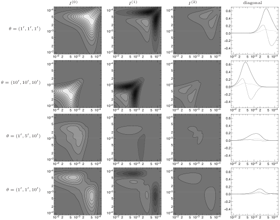
Figure 1: The filter functions $I^{(m)}$ (16) for the generalized third-order aperture mass statistics as a function of the bispectrum (15). Contours of the $I^{(m)}$ for $m=0,1,2$ from left to right are plotted for different values of $\theta_{i}$ as a function of $\ell_{1}$ and $\ell_{2}$ (in units of inverse radians). The dashed contours indicate negative values. The right-most panels show the profile along the diagonal of $I^{(m)}$, where the solid, dashed and dotted lines correspond to $m=0,1$ and 2 respectively.

The second- and third-order aperture mass statistics can be calculated as integrals over the power spectrum and the bispectrum of the convergence $\kappa$, respectively. For second order, we have

$$\left\langle{M_{\rm ap}^{2}(\theta)}\right\rangle=\int\frac{{\mathrm{d}}\ell\,\ell}{2\pi}P_{\kappa}(\ell)\hat{U}^{2}(\theta\ell),$$ (11)

where $\hat{U}(\theta\ell)={\cal F}[U_{\theta}](\ell)=(\theta\ell)^{2}/2\cdot\exp[-(\theta\ell)^{2}/2]$ is the Fourier transform of the filter function $U_{\theta}$. The generalized third-order aperture mass statistics can be written as

$$\left\langle{M_{\rm ap}^{3}(\theta_{1},\theta_{2},\theta_{3})}\right\rangle\equiv\langle M_{\rm ap}(\theta_{1})M_{\rm ap}(\theta_{2})M_{\rm ap}(\theta_{3})\rangle$$ (12)

$$= \int\frac{{\mathrm{d}}^{2}\ell_{1}}{(2\pi)^{2}}\int\frac{{\mathrm{d}}^{2}\ell_{2}}{(2\pi)^{2}}\,B_{\kappa}(\@vec{\ell}_{1},\@vec{\ell}_{2})$$

$$\times\sum\limits_{(i,j,k)\in S_{3}}\hat{U}(\theta_{i}|\@vec{\ell}_{1}|)\,\hat{U}(\theta_{j}|\@vec{\ell}_{2}|)\,\hat{U}(\theta_{k}|\@vec{\ell}_{1}+\@vec{\ell}_{2}|),$$

where $S_{3}$ is the symmetric permutation group of $(123)$, thus the summation is performed over even permutations of $i,j,k$ (Schneider et al. 2004).

Both integrals (11) and (12) are easily calculated numerically due to the exponential cut-off of $\hat{U}$ for large $\ell$. Eq. (12) can be simplified further if the bispectrum can be factorized as in (2). Then, terms of the form

$$K^{(m)}(\theta\ell_{1},\theta\ell_{2})=$$ (13)

$$\hskip 20.00003pt\int\limits_{0}^{2\pi}{\mathrm{d}}\varphi\cos^{m}(\varphi)\,\hat{U}\left(\theta\sqrt{\ell_{1}^{2}+\ell_{2}^{2}+2\ell_{1}\ell_{2}\cos\varphi}\right),$$

for $m=0,1,2$ can be separated and carried out analytically,

$$K^{(0)}(t_{1},t_{2}) = \pi{\rm e}^{-\frac{1}{2}(t_{1}^{2}+t_{2}^{2})}\left[(t_{1}^{2}+t_{2}^{2}){\rm I}_{0}(t_{1}t_{2})-2t_{1}t_{2}{\rm I}_{1}(t_{1}t_{2})\right],$$

$$K^{(1)}(t_{1},t_{2}) = \pi{\rm e}^{-\frac{1}{2}(t_{1}^{2}+t_{2}^{2})}\left[2t_{1}t_{2}{\rm I}_{0}(t_{1}t_{2})\right.$$ (14)

$$\left.-(2+t_{1}^{2}+t_{2}^{2}){\rm I}_{1}(t_{1}t_{2})\right]$$

$$K^{(2)}(t_{1},t_{2}) = \pi{\rm e}^{-\frac{1}{2}(t_{1}^{2}+t_{2}^{2})}\bigg{[}(2+t_{1}^{2}+t_{2}^{2}){\rm I}_{0}(t_{1}t_{2})$$

$$\left.-\left(\frac{t_{1}^{2}+t_{2}^{2}+4}{t_{1}t_{2}}+2t_{1}t_{2}\right){\rm I}_{1}(t_{1}t_{2})\right],$$

where ${\rm I}_{n}$ is the modified Bessel function of order $n$. We get for (12)

$$\left\langle{M_{\rm ap}^{3}(\theta_{1},\theta_{2},\theta_{3})}\right\rangle=(2\pi)^{-3}\int{\mathrm{d}}\ell_{1}\,\ell_{1}\int{\mathrm{d}}\ell_{2}\,\ell_{2}$$ (15)

$$\hskip 30.00005pt\times\sum_{m=0}^{2}I^{(m)}(\theta_{1},\theta_{2},\theta_{3};\ell_{1},\ell_{2})\,\bar{b}_{\kappa}^{(m)}(\ell_{1},\ell_{2}),$$

with

$$I^{(m)}(\theta_{1},\theta_{2},\theta_{3};\ell_{1},\ell_{2})=F_{2}^{(m)}(\ell_{1},\ell_{2})$$ (16)

$$\hskip 30.00005pt\times\sum\limits_{(i,j,k)\in S_{3}}\hat{U}(\theta_{i}\ell_{1})\,\hat{U}(\theta_{j}\ell_{2})K^{(m)}(\theta_{k}\ell_{1},\theta_{k}\ell_{2}).$$

One sees in Fig. 1 that the functions $I^{(m)}$ as defined in the previous equation are relatively well localized which makes $\langle M_{\rm ap}^{3}\rangle$ a local measure of the bispectrum. Further, for equal filter scales, only the region around the diagonal of the $\bar{b}_{\kappa}^{(m)}$ is probed, corresponding to equilateral triangles in Fourier space. When different filter scales are taken into account, other parts further away from the diagonal of $\bar{b}_{\kappa}^{(m)}$ can contribute to the integral. Although in this latter case the amplitude of $I^{(m)}$ is lower, the generalized aperture mass, probing the bispectrum for general triangles in Fourier space, contains much more information about the bispectrum and cosmology than the ‘diagonal’ one. This approach to sample the bispectrum on a large region of Fourier space is similar to a previous study (Takada & Jain 2004), who have used all triangle configurations of the convergence bispectrum in order to predict tight constraints on cosmological parameters from cosmic shear. In contrast to that work, we use moments of the aperture mass statistics (which are direct weak lensing observables) as real-space probes of the convergence power spectrum and bispectrum.

3.3 Ray-tracing simulations

We use 36 $\Lambda$CDM ray-tracing simulations, kindly provided by T. Hamana (for more details see Ménard et al. 2003) in order to calculate the second- and third-order aperture mass statistics and their covariances (Sect. 4) . Each field consists of $1024^{2}$ data points in $\kappa$ and $\gamma$, the pixel size is $0.2^{\prime}$. We assume our galaxies to be given on a regular grid – every pixel corresponds to a galaxy, thus our source galaxy density is 25 per square arc minute. We note here that the Poisson noise is much smaller than the shape noise of the ellipticities, and that apertures with radii smaller than one arc minute are discarded due to discreteness effects in the ray-tracing and in the underlying $N$-body simulations.

All source galaxies are located at a redshift of about unity. See Table 1 for the fiducial values of the parameters.

Table 1: Fiducial values of the cosmological parameters that are used for the theoretical model to match the ray-tracing simulations. If the shape parameter $\Gamma$ is interpreted as Sugiyama’s $\Gamma$ (Sugiyama 1995), our fiducial model corresponds to $\Omega_{\rm b}=0.04$ and $h=0.7$.

$\Omega_{\rm m}$	$\Omega_{\Lambda}$	$\Gamma$	$\sigma_{8}$	$n_{\rm s}$	$z_{0}$
0.3	0.7	0.1723	0.9	1.0	0.9772

Figure 2: $\langle M_{\rm ap}^{2}\rangle$ and $\langle M_{\rm ap}^{3}\rangle$ from the 36 $\Lambda$CDM simulations (solid lines) as compared to theoretical predictions (dashed and dotted lines). The error bars are the rms values from the 36 fields. $\langle M_{\rm ap}^{3}\rangle$ is calculated from the simulations for aperture radii smaller than one sixth of the field size. PD = Peacock & Dodds (1996), HEPT = Scoccimarro & Couchman (2001), PT = (quasi-)linear perturbation theory.

Because the field $\kappa$ is given on a regular grid, moments of the aperture mass statistics (8) can be calculated very quickly using FFT, with the ensemble averages replaced by the average over all aperture centers $\@vec{\vartheta}$. However, since for discrete Fourier transforms, periodic boundary conditions are assumed, which is not the case for the ray-tracing simulations, points near the borders have to be excluded from the averaging. This leads to smaller effective area and therefore to an overestimation of the covariance of the $M_{\rm ap}$-statistics, which increases with the aperture radius. In order to avoid this, one could calculate $\langle M_{\rm ap}^{2}\rangle$ and $\langle M_{\rm ap}^{3}\rangle$ from the shear correlation functions, which takes into account the complete area. This approach is not chosen here because of the time-consuming calculation of the 3PCF. The correction scheme we apply to the covariance matrices is described in Sect. 4.1.

Figs. 2 and 3 show $\langle M_{\rm ap}^{2}\rangle$ and $\langle M_{\rm ap}^{3}\rangle$ from the $\Lambda$CDM simulations and the theoretical predictions based on HEPT. The non-linear fitting formulae reproduce reasonably well the results from the simulations for angular scales above $\sim$ 1 arc minute. The largest aperture which can be put onto the field without being too close to the border is for $\theta_{\rm max}=a/6=34^{\prime}$, where $a=204.8^{\prime}$ is the field size.

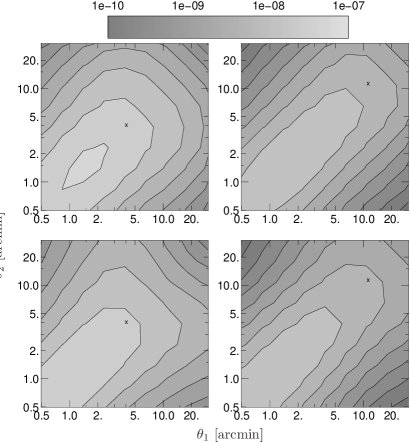
Figure 3: Contours of $\langle M_{\rm ap}^{3}(\theta_{1},\theta_{2},\theta_{3})\rangle$ from simulations (upper row) and from the HEPT model (lower row). In each panel $\theta_{3}$ is fixed to the value indicated by the cross. These are 3.87 arc minutes (left column) and 10.77 arc minutes (right column).

For comparison, we calculate $\langle M_{\rm ap}^{3}\rangle$ by integrating over the 3PCF, using eqs. (62) and (71) from Schneider et al. (2004). Although we use the fast tree-code algorithm of Jarvis et al. (2004) to calculate the 3PCF, it is still very time-taking since a fine binning of the 3PCF is needed (see below). Our results are shown in Fig. 4 and represent the average over three of the ray-tracing fields. $\langle M_{\rm ap}^{3}\rangle$ as calculated via apertures cannot be determined for large radii because of the border effects, as mentioned above. Since $\langle M_{\rm ap}^{3}\rangle$ obtained via integrating over the 3PCF is based on the simulated shear field, we use the $\gamma$ fields instead of the $\kappa$ fields in order to calculate $\langle M_{\rm ap}^{3}\rangle$ via the FFT aperture method, using the second equality in (8). With $M_{\perp}(\theta)=\Im\left(Q^{\prime}_{\theta}*\gamma\right)$, we also determine the statistics $\langle M_{\rm ap}^{2}M_{\perp}\rangle$, $\langle M_{\rm ap}M_{\perp}^{2}\rangle$ and $\langle M_{\perp}^{3}\rangle$ as indicators of a B-mode. $\langle M_{\rm ap}M_{\perp}^{2}\rangle$ is expected to vanish if the ray-tracing simulations are B-mode-free. The two quantities with odd power in $M_{\perp}$ can only be non-zero for a convergence field which is not parity-invariant (Schneider 2003). We found all three statistics to be three and more orders of magnitude below the pure E-mode, confirming that the ray-tracing simulations contain virtually no B-mode and are parity-invariant. However, when inferred from the 3PCF, $\langle M_{\rm ap}M_{\perp}^{2}\rangle$ is at a couple of percent of the E-mode. This is most probable due to the binning of the 3PCF — the B-mode gets smaller when we refine the binning. In our calculations, we use a logarithmic bin width of $b=0.075$. As can be seen in Fig. 4, there is good agreement between the two methods, except for very small angular scales (where the B-mode is of the order 10%) and large aperture radii (where a significant fraction of the field near the border can not be taken into account with the aperture method).

Figure 4: $\langle M_{\rm ap,d}^{3}\rangle(\theta)$ from apertures (bold line), and from the integration over the 3PCF (thin line). Also plotted are the B-mode signals from the integration method $\langle M_{\rm ap}M_{\perp}^{2}\rangle$ (dashed), $\langle M_{\rm ap}^{2}M_{\perp}\rangle$ (dotted) and $\langle M_{\perp}^{3}\rangle$ (dash-dotted). The curves represent the mean from three of the ray-tracing fields.

Integrating over the 3PCF is the preferred method in the case of real data, since the determination of correlation functions is not affected by unusable regions which makes placing apertures onto the observed field very ineffective. However, the calculation of the 3PCF is very time-consuming even using the fast tree-code algorithm. Moreover, a relatively fine binning of the 3PCF is needed in order not to introduce a B-mode from the integration of the 3PCF, and the computation time goes as $b^{-3.3}$ (Jarvis et al. 2004) where $b$ is the logarithmic bin width. With $b=0.075$, the integration method takes about a factor 500 longer than the aperture method using FFT.

3.4 Dependence on cosmological parameters

The goal of this paper is to study the ability of weak lensing measurements of the aperture mass statistics to constrain cosmological parameters. It is therefore instructive to show the dependence of the aperture mass on various cosmological parameters, and to compare its second- and third-order moments. The more different the dependencies are for the second- and third-order statistics, the better will be the improvement on the parameter constraints when combining both.

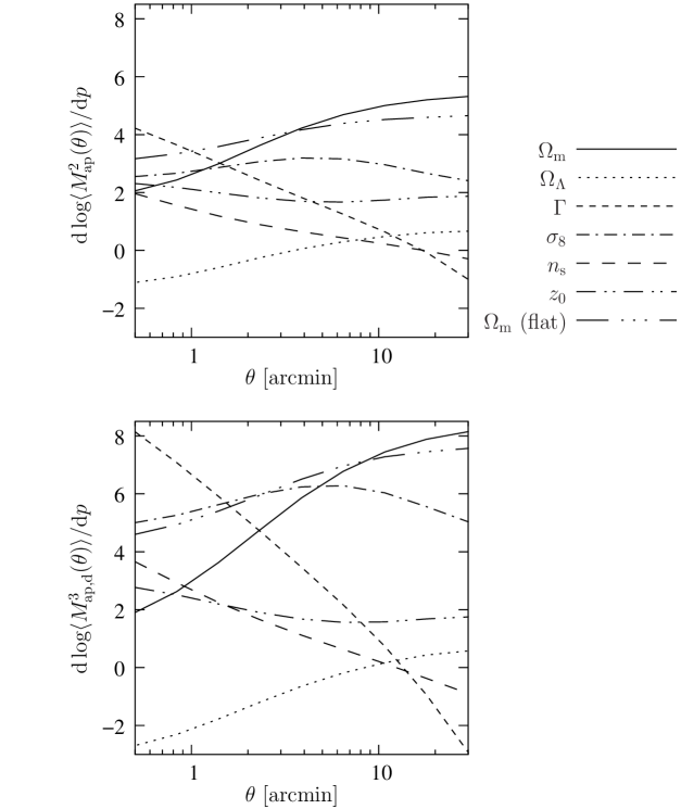
Figure 5: Logarithmic derivatives of $\langle M_{\rm ap}^{2}\rangle$ and $\langle M_{\rm ap,d}^{3}\rangle$ with respect to some cosmological parameters as indicated in the figure legend.

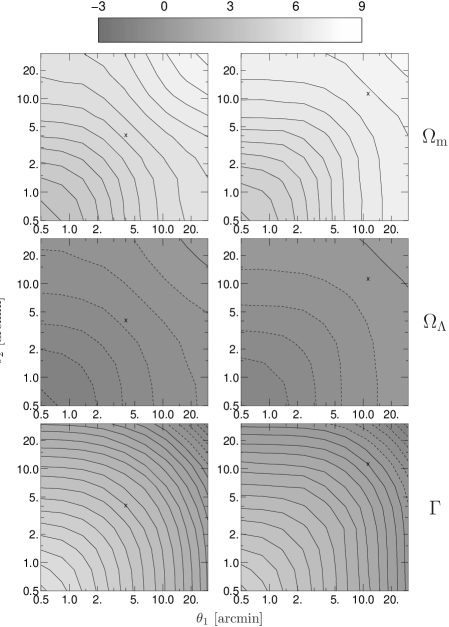
Figure 6: Contours of ${\mathrm{d}}\log\langle M_{\rm ap}^{3}(\theta_{1},\theta_{2},\theta_{3})\rangle/{\mathrm{d}}p$ from the HEPT model, with $p=\Omega_{\rm m},\Omega_{\Lambda},\Gamma$ from top to bottom. In each panel $\theta_{3}$ is fixed to the value indicated by the cross. These are 3.87 (left column) and 10.77 arcminutes (right column).

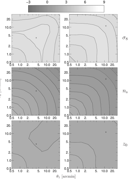
Figure 7: Contours of ${\mathrm{d}}\log\langle M_{\rm ap}^{3}(\theta_{1},\theta_{2},\theta_{3})\rangle/{\mathrm{d}}p$ from the HEPT model, with $p=\sigma_{8},n_{\rm s},z_{0}$ from top to bottom. In each panel $\theta_{3}$ is fixed to the value indicated by the cross. These are 3.87 (left column) and 10.77 arcminutes (right column).

In Figs. 5 - 7, the logarithmic derivatives of the aperture mass statistics with respect to cosmological parameters used here are shown. In all cases, the curves shown in Fig. 5 are quite featureless, their similarity is due to the near-degeneracies between the parameters. For example, we find that the ratios ($\partial\langle M_{\rm ap}^{2}\rangle/\partial n_{\rm s})/(\partial\langle M_{\rm ap}^{2}\rangle/\partial\Gamma)$ $\approx$ $(\partial\langle M_{\rm ap,d}^{3}\rangle/\partial n_{\rm s})/(\partial\langle M_{\rm ap,d}^{3}\rangle/\partial\Gamma)$ are roughly equal and constant as a function of the aperture radius $\theta$. Therefore, we expect these two parameters to have the same near-degeneracy for both statistics.

The ratio of derivatives with respect to $\Omega_{\rm m}$ and $\sigma_{8}$ are slowly increasing functions of $\theta$, with significant differences between $\langle M_{\rm ap}^{2}\rangle$ and $\langle M_{\rm ap,d}^{3}\rangle$. From that we can infer that the reduced skewness $s_{3}=\langle M_{\rm ap,d}^{3}\rangle/\langle M_{\rm ap}^{2}\rangle^{2}$ breaks the $\Omega_{\rm m}$ - $\sigma_{8}$ degeneracy of second-order cosmic shear statistics. From Fig. 5 one sees that $\partial\log\langle M_{\rm ap,d}^{3}\rangle/\partial\sigma_{8}\approx 2\partial\log\langle M_{\rm ap}^{2}\rangle/\partial\sigma_{8}$, so $\partial s_{3}/\partial\sigma_{8}\approx 0$ — $s_{3}$ is indeed nearly independent of $\sigma_{8}$, as predicted from quasi-linear perturbation theory (Bernardeau et al. 1997; Schneider et al. 1998).

4 Covariance matrices of aperture mass statistics

4.1 Definition and Notation

Let $M_{i}$ be an estimator of some statistics, e.g. of the second-order aperture mass $\langle M_{\rm ap}^{2}(\theta_{i})\rangle$ for some aperture radius $\theta_{i}$. The covariance matrix of this estimator is defined as

$${\rm Cov}(M)_{ij}=\left\langle{M_{i}M_{j}}\right\rangle-\big{\langle}{M_{i}}\big{\rangle}\left\langle{M_{j}}\right\rangle.$$ (17)

In case of the generalized third-order aperture mass $\langle M_{\rm ap}^{3}(\theta_{i},\theta_{j},\theta_{k})\rangle$, the covariance depends on six scalar quantities, namely the $2\times 3$ filter scales involved. In order to obtain a two-dimensional matrix, we relabel all non-degenerate combinations of filter triplets ($\langle M_{\rm ap}^{3}\rangle$ is invariant under permutations of its arguments) with a single index. The resulting $\langle M_{\rm ap}^{3}(\theta_{1},\theta_{2},\theta_{3})\rangle$-vector is organized such that $(\theta_{1},\theta_{2},\theta_{3})$ is in lexical order, we further demand that $\theta_{1}\leq\theta_{2}\leq\theta_{3}$. Note that the labeling order does not play a role in the later analysis. For a number of $N$ distinct filter scales, there are ${N+2\choose 3}=N(N+1)(N+2)/6$ different combinations.

We define the two covariance matrices ${\hbox{$Cov$}}(M_{\rm ap}^{2})$ and ${\hbox{$Cov$}}(M_{\rm ap}^{3})$ for the second- and generalized third-order aperture mass statistics, respectively. Further, for the skewness of $M_{\rm ap}$, which is a function of only one filter scale, $M_{\rm ap,d}^{3}(\theta)\equiv M_{\rm ap}^{3}(\theta,\theta,\theta)$, we define the covariance matrix ${\hbox{$Cov$}}(M_{\rm ap,d}^{3})$.

The averaging in eq. (17) is performed over the different simulations. Because of the small number of realizations, we split up each of the 36 fields into 4 subfields, corresponding to a survey of area $A=102.4^{\prime 2}$, and average over the resulting 144 subfields. Adjacent subfields do not represent fully independent realizations of the convergence field, but the correlations are negligible: when averaging over only a bootstrapped subset of subfields, we get no systematic deviation but only a noisier estimate of the covariance. Note that because of the splitting, the maximum usable aperture radius is now 17 arc minutes.

We take into account apertures with centers not closer to the border than three times the aperture radius $\theta$. This results in an effective area $A_{\rm eff}(\theta)$ which is smaller than the original area $A=a^{2}$, namely $A_{\rm eff}(\theta)=(a-6\theta)^{2}$. Since the covariance is anti-proportional to the observed area, we can easily apply a correction scheme, and multiply each covariance matrix entry ${\rm Cov}(\theta_{1},\theta_{2})$ by $\sqrt{A_{\rm eff}(\theta_{1})A_{\rm eff}(\theta_{2})}/A$ in the case of $\langle M_{\rm ap}^{2}\rangle$ and $\langle M_{\rm ap,d}^{3}\rangle$. For the generalized third-order aperture mass, where each matrix element corresponds to two triplets of aperture radii, the effective area corresponding to the maximum radius of each triplet is inserted into the correction factor. This correction makes sure that the covariance matrix corresponds to the same survey area $A$ for all aperture radii.

For the Fisher matrix analysis of constraints on cosmological parameters (Sect. 5), we scale the covariances, obtained from the 2.9 square degree fields, to a corresponding survey area of 29 square degree, by dividing them by 10, making use of their $1/A$-dependence. Note that this increase of survey area is not equivalent of extending a single patch on the sky, since this additional observed area will not sample independent but correlated parts of the large-scale structure and the decrease in cosmic variance will be less than the increase in area. Our scaling of the area corresponds to observing 10 independent lines of sight, each one 2.9 square in area.

4.2 Adding intrinsic ellipticities

In order to realistically model the noise coming from the intrinsic ellipticities of the source galaxies, one would have to add a random ellipticity to each shear value. It has been shown that this is equivalent to adding a noise term to the convergence $\kappa$ (van Waerbeke 2000). For mass reconstructions, this noise has to be added to a smoothed $\kappa$ map, however, in our case, no smoothing is required, thus, to each pixel of $\kappa$ we add a random Gaussian variable with dispersion $\sigma_{\varepsilon}=0.3/\sqrt{2}$. In the case of $\langle M_{\rm ap}^{2}\rangle$, this yields the predicted amplitude to the variance without need of smoothing, as can be seen in Fig. 8. The shot-noise contribution to the variance is in good agreement with the Monte-Carlo method from Kilbinger & Schneider (2004).

The shot-noise term of the variance of $M_{\rm ap}^{3}$ agrees very well with the analytical expectation (30), except for large $\theta$, where only few apertures can be placed onto the field which are not too close to the border. Apparently, adding intrinsic random ellipticities to each grid point without smoothing introduces no artefacts.

4.3 Gaussianized fields

For Gaussian random fields, Schneider et al. (2002) found analytic expressions for the covariance of ${M_{\rm ap}^{2}}$, which were integrated via a Monte-Carlo method by Kilbinger & Schneider (2004). In order to compare the results presented in this work with the Monte-Carlo approach as a sanity check, we transform the ray-tracing simulations into Gaussian fields without changing the power spectrum. This is achieved by multiplying the Fourier transform $\hat{\kappa}$ of each convergence field by random phases (destroying the phase correlations). Then for each Fourier mode $\@vec{k}$, we pick a $\hat{\kappa}(\@vec{k})$ value randomly from one of the 36 fields.

Destroying the phase correlations for each individual field independently would not have led to the desired goal. Randomizing the phases cancels the connected 4-point term (kurtosis) of each individual realization, but not the kurtosis of the underlying ensemble. Our estimator of the covariance is independent of the kurtosis of each individual realization, because we first determine $\langle M_{\rm ap}^{2}\rangle$ for each field and then average the square of this quantity over all fields – thus for this averaging, only second-order quantities are taken into account. The process of remixing the $\hat{\kappa}$-fields in Fourier space annihilates the kurtosis of the underlying ensemble, and the resulting fields represent realizations of a Gaussian random field.

In Fig. 8, the variance (diagonal of the covariance) of $M_{\rm ap}^{2}$ is plotted. The results from this work are in fairly good agreement with the Kilbinger & Schneider (2004) Monte-Carlo method, although the cosmic variance term from the ray-tracings is slightly higher than the one from the Monte-Carlo method.

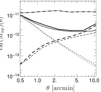
Figure 8: The variance of $\langle M_{\rm ap}^{2}\rangle$ from the Gaussianized $\Lambda$CDM simulations (bold lines), in comparison with the Monte-Carlo method from Kilbinger & Schneider (2004) (thin lines), for a survey area of $A={102.4^{\prime}}^{2}$. The dotted lines give the variance from shot noise only (due to the intrinsic ellipticity dispersion), the dashed curves correspond to cosmic variance only. The solid line include both error sources; note that it is not the sum of the other two curves – there is a non-vanishing mixed term. The dash-dotted line indicates the cosmic variance term for the non-Gaussian case.

Figure 9: Contour plots of the cosmic-variance-only term of the covariance of ${M_{\rm ap}^{2}}$, for the Monte-Carlo method (upper left panel), the Gaussianized ray-tracing fields (upper right) and the original fields (lower panel), for a survey area of $A={102.4^{\prime}}^{2}$. The contours are logarithmically spaced.

It is clear from this figure that non-Gaussianity increases the noise level on the diagonal by an enormous amount, about two orders of magnitude at $\sim 1^{\prime}$. The ratio of the non-Gaussian to the Gaussian variance is $\propto\theta^{-2}$ for small $\theta$ and gets less steep for larger $\theta$.

On nearly all scales, cosmic variance dominates the shot noise. From Fig. 9, we see that due to mode-coupling, high cross-correlations between different angular scales are introduced, present on the off-diagonal of the covariance.

4.4 The case of $\langle M_{\rm ap}^{3}\rangle$

As for the second-order case, the variance of the aperture mass skewness, ${\rm var}(M_{\rm ap,d}^{3}(\theta))={\rm var}(M_{\rm ap}^{3}(\theta,\theta,\theta))$ is dominated by cosmic variance which is larger than the shot noise on all but very small scales.

The covariance matrix of ${M_{\rm ap}^{3}}$ is not diagonal-dominant, and shows a self-similar pattern with many secondary diagonals, originating from the reordering of $\langle M_{\rm ap}^{3}(\theta_{1},\theta_{2},\theta_{3})\rangle$ into a single vector, which inevitably creates repeating entries of similar combinations of aperture radii. The correlation of $\langle M_{\rm ap}^{2}\rangle$ for two aperture radii $\theta_{1}\geq\theta_{2}$ is a quickly decreasing function of the ratio $\theta_{1}/\theta_{2}$. In the case of $\langle M_{\rm ap}^{3}\rangle$ however, there are many combinations of filter scales which show a high correlation. This fact together with the small sample of realizations of $\kappa$-fields causes the covariance matrix to be very ill-conditioned. For our Fisher matrix analysis (Sect. 5.2), we have to invert the covariance matrix. We find stable results for the matrix inverting when the ratio of adjacent aperture radii is chosen not to be too small, i.e. larger than about 1.5.

One way to determine whether our estimate of the covariance of ${M_{\rm ap}^{3}}$ is reasonable would involve 6-point statistics, which is not feasible analytically. Instead, we slightly modify the aperture radii used in the analysis and get a rough estimate of the accuracy of this method. We comment on the stability of our results in Sect. 5.5.

5 Constraints on cosmological parameters

From the simulated data, we “observe” a data vector $\@vec{M}$, which in our case consists of the values of $\langle M_{\rm ap}^{2}\rangle$ and/or $\langle M_{\rm ap}^{3}\rangle$ as a function of angular scales. Using a theoretical model, and approximating our observables as Gaussian variables, we construct a likelihood function ${\cal L}(\@vec{M};\@vec{p})$, which depends on a number of model parameters $\@vec{p}=(p_{1},p_{2},\ldots,p_{n})$. The likelihood is ${\cal L}\propto\exp(-\chi^{2}/2)$ with

$$\chi^{2}(\@vec{M};\@vec{p})=\hbox to0.0pt{$\displaystyle\sum_{kl}\left(M_{k}(\@vec{p})-M_{k}(\@vec{p}_{0})\right)({\rm Cov}^{-1})_{kl}$\hss}$$ (18)

$$\times\left(M_{l}(\@vec{p})-M_{l}(\@vec{p}_{0})\right).$$

where the indices $k$ and $l$ run over the individual data points.

5.1 The input data

We distinguish the following five cases for the input data vector $\@vec{M}$ and its covariance $Cov$:

1. (‘2’) $M_{l}=\langle M_{\rm ap}^{2}(\theta_{l})\rangle$, $Cov$ = covariance of $M_{\rm ap}^{2}$.

2. (‘3’) $M_{l}=\langle{M_{\rm ap,d}^{3}(\theta_{l})}\rangle$, $Cov$ = covariance of $M_{\rm ap,d}^{3}$.

3. (‘3d’) $M_{l}=\langle M_{\rm ap}^{3}(\theta_{i},\theta_{j},\theta_{k})\rangle$ for a combination of three filter radii which after relabeling corresponds to index $l$ as described in Sect. 4.1. $Cov$ = covariance of $M_{\rm ap}^{3}$.

4. (‘2+3d’) $M_{l}=$ some element from the concatenated data vector containing $\langle M_{\rm ap}^{2}\rangle$ and $\langle M_{\rm ap,d}^{3}\rangle$. $Cov$ is a block matrix containing the covariances of $M_{\rm ap}^{2}$ and ${M_{\rm ap,d}^{3}}$ on the diagonal and the cross-correlation on the off-diagonal.

5. (‘2+3’) $M_{l}=$ some element from the concatenated data vector containing $\langle M_{\rm ap}^{2}\rangle$ and $\langle M_{\rm ap}^{3}\rangle$. $Cov$ is a block matrix containing the covariances of $M_{\rm ap}^{2}$ and ${M_{\rm ap}^{3}}$ on the diagonal and the cross-correlation on the off-diagonal.

Our choice of the survey geometry corresponds to ten uncorrelated fields, each of size $A=102.4^{\prime 2}$. In order to get the covariances of the aperture mass statistics, we split each of the 36 ray-tracing simulations into four subfields and calculate the rms over the 144 resulting fields. We devide the resulting covariance matrices by a factor of 10, which then correspond to a total survey area of $A=10\cdot 102.4^{\prime 2}=29$ square degree. We use six different filter radii, logarithmically spaced between 1 and 15 arc minutes and thus have six data points for each of $\langle M_{\rm ap}^{2}\rangle$ and $\langle M_{\rm ap,d}^{3}\rangle$ and 56 for $\langle M_{\rm ap}^{3}\rangle$.

5.2 Fisher matrix

It would be desirable to calculate the full $n$-dimensional likelihood function in order to make predictions about error bars and directions of degeneracies between parameters. This, however, is extremely time-consuming even for sparse sampling in parameter space, because for every $\@vec{p}$, the bispectrum and the aperture mass statistics have to be calculated involving three-dimensional integrals.

Instead, we use the Fisher information matrix (Kendall & Stuart 1969; Tegmark et al. 1997) which gives us a local description of the likelihood ${\cal L}$ at its maximum. The Fisher matrix is defined as

$$\vec{F}_{ij}=\left\langle\frac{\partial^{2}[-\ln\cal L]}{\partial p_{i}\partial p_{j}}\right\rangle=\left(\frac{\partial^{2}[-\ln\cal L]}{\partial p_{i}\partial p_{j}}\right)_{\@vec{p}=\@vec{p}_{0}},$$ (19)

where $\@vec{p}_{0}$ denotes the “true” parameter values, in our case the input parameters of the simulations, see Table 1. The second equality in (19) holds if the maximum likelihood estimator of $\@vec{p}_{0}$ is unbiased. The Fisher matrix is the expectation value of the Hessian matrix of $({-\ln\cal L})$ at $\@vec{p}=\@vec{p}_{0}$, which in the case of an unbiased maximum likelihood estimator coincides on average with $\cal L$’s maximum – thus it is a measure of how fast ${\cal L}$ falls off from the maximum.

The smallest possible variance $\sigma$ of any unbiased estimator of some parameter $p_{i}$ is given by the Cramér-Rao inequality

$$\sigma(p_{i})\geq\sqrt{(F^{-1})_{ii}}\;;$$ (20)

the expression on the right-hand side is called the minimum variance bound (MVB).

Under the assumption that the parameter dependence of the covariance can be neglected, we get from eq. (18) and (19):

$$F_{ij}=\sum_{kl}\left(\frac{\partial M_{k}}{\partial p_{i}}\right)\left({\rm Cov}^{-1}\right)_{kl}\left(\frac{\partial M_{l}}{\partial p_{j}}\right).$$ (21)

The derivatives of the aperture mass statistics with respect to the parameters $p_{i}$ are calculated numerically from the HEPT model, using polynomial extrapolation of finite differences (Press et al. 1992). The Fisher matrix for the four combinations of second- and third-order statistics considered in this work is given in Table 2.

Table 2: Fisher matrix for the five different input data as listed in Sect. 5.1, denoted by ‘2’, ‘3’, ‘3d’, ‘2+3d’ and ‘2+3’, respectively. The survey is 29 square degree, all entries are given in units of $10^{4}$.

		$\Omega_{\rm m}$	$\Omega_{\Lambda}$	$\Gamma$	$\sigma_{8}$	$n_{\rm s}$	$z_{0}$
	$\Omega_{\rm m}$	$1.766$	$-0.268$	$1.543$	$1.597$	$0.601$	$1.079$
	$\Omega_{\Lambda}$	$-0.268$	$0.239$	$-0.784$	$-0.424$	$-0.336$	$-0.413$
	$\Gamma$	$1.543$	$-0.784$	$2.875$	$1.905$	$1.202$	$1.630$
2	$\sigma_{8}$	$1.597$	$-0.424$	$1.905$	$1.618$	$0.766$	$1.200$
	$n_{\rm s}$	$0.601$	$-0.336$	$1.202$	$0.766$	$0.507$	$0.674$
	$z_{0}$	$1.079$	$-0.413$	$1.630$	$1.200$	$0.674$	$0.975$
	$\Omega_{\rm m}$	$1.698$	$-0.315$	$1.260$	$1.848$	$0.478$	$0.661$
	$\Omega_{\Lambda}$	$-0.315$	$0.445$	$-1.304$	$-0.852$	$-0.552$	$-0.452$
	$\Gamma$	$1.260$	$-1.304$	$3.952$	$2.803$	$1.653$	$1.389$
3	$\sigma_{8}$	$1.848$	$-0.852$	$2.803$	$2.705$	$1.137$	$1.146$
	$n_{\rm s}$	$0.478$	$-0.552$	$1.653$	$1.137$	$0.701$	$0.579$
	$z_{0}$	$0.661$	$-0.452$	$1.389$	$1.146$	$0.579$	$0.544$
	$\Omega_{\rm m}$	$0.263$	$-0.079$	$0.291$	$0.342$	$0.109$	$0.119$
	$\Omega_{\Lambda}$	$-0.079$	$0.146$	$-0.422$	$-0.255$	$-0.177$	$-0.141$
	$\Gamma$	$0.291$	$-0.422$	$1.236$	$0.794$	$0.513$	$0.418$
3d	$\sigma_{8}$	$0.342$	$-0.255$	$0.794$	$0.635$	$0.319$	$0.284$
	$n_{\rm s}$	$0.109$	$-0.177$	$0.513$	$0.319$	$0.214$	$0.173$
	$z_{0}$	$0.119$	$-0.141$	$0.418$	$0.284$	$0.173$	$0.144$
	$\Omega_{\rm m}$	$3.256$	$-0.071$	$1.844$	$2.322$	$0.713$	$1.757$
	$\Omega_{\Lambda}$	$-0.071$	$0.363$	$-0.999$	$-0.466$	$-0.434$	$-0.379$
	$\Gamma$	$1.844$	$-0.999$	$3.613$	$2.405$	$1.527$	$1.924$
2+3d	$\sigma_{8}$	$2.322$	$-0.466$	$2.405$	$2.180$	$0.974$	$1.592$
	$n_{\rm s}$	$0.713$	$-0.434$	$1.527$	$0.974$	$0.653$	$0.799$
	$z_{0}$	$1.757$	$-0.379$	$1.924$	$1.592$	$0.799$	$1.337$
	$\Omega_{\rm m}$	$7.046$	$0.348$	$2.457$	$4.440$	$0.939$	$3.219$
	$\Omega_{\Lambda}$	$0.348$	$0.764$	$-1.775$	$-0.740$	$-0.773$	$-0.435$
	$\Gamma$	$2.457$	$-1.775$	$5.846$	$3.925$	$2.486$	$2.756$
2+3	$\sigma_{8}$	$4.440$	$-0.740$	$3.925$	$4.162$	$1.597$	$2.635$
	$n_{\rm s}$	$0.939$	$-0.773$	$2.486$	$1.597$	$1.076$	$1.159$
	$z_{0}$	$3.219$	$-0.435$	$2.756$	$2.635$	$1.159$	$2.169$

5.3 Minimum Variance Bounds (MVBs)

For various combinations of cosmological parameters, we compute the MVBs from the Fisher information matrix (21). As the covariance scales with $A^{-1}$ (where $A$ is the observed area), the MVB is roughly proportional to $1/\sqrt{A}$. First, the analysis is done for only two parameters, in order to graphically display the MVBs. Then, simultaneous MVBs for three and more parameters are calculated.

5.3.1 Two parameters

In Fig. 10, we show the MVBs as ellipses in two-dimensional subspaces of the parameter space. The hidden parameters are fixed. In all cases, the combination of $\langle M_{\rm ap}^{2}\rangle$ and $\langle M_{\rm ap}^{3}\rangle$ leads to a substantial reduction in the 1-$\sigma$-error. As expected, the generalized third-order aperture mass statistics yields much better constraints than the ‘diagonal’ version $\langle{M_{\rm ap,d}^{3}}\rangle$. The direction of degeneracy is slightly different for some parameter pairs, most notably when the source redshift parameter $z_{0}$ is involved, making the combination of the statistics very effective in these cases. The $\Omega_{\rm m}$-$\sigma_{8}$-degeneracy is lifted partially and the combined Fisher matrix analysis yields a large improvement on the error of the two parameters. Contrary to that, the pair $(\Gamma,n_{\rm s})$ is degenerate to a high level for both $\langle M_{\rm ap}^{2}\rangle$ and $\langle M_{\rm ap}^{3}\rangle$ as well as for their combination.

Note that the combined 1-$\sigma$-errors are not completely determined by the product of the likelihoods of $\langle M_{\rm ap}^{2}\rangle$ and $\langle M_{\rm ap}^{3}\rangle$. The combined covariance is not the direct product of the covariances of $\langle M_{\rm ap}^{2}\rangle$ and $\langle M_{\rm ap}^{3}\rangle$ because of the contribution from the cross-correlation between both statistics.

It is not surprising that the directions of degeneracy between parameters are more or less similar for $\langle M_{\rm ap}^{2}\rangle$ and $\langle M_{\rm ap}^{3}\rangle$, with larger differences existing when $z_{0}$ is one of the free parameters. Both statistics depend on the convergence power spectrum, because in HEPT as well as in quasi-linear PT, the bispectrum of the matter fluctuations is given in terms of the power spectrum (3). The differences between $\langle M_{\rm ap}^{2}\rangle$ and $\langle M_{\rm ap}^{3}\rangle$ mainly come from their different dependence on the projection prefactor and the lens efficiency $G$ (eq. 4). The projection is most sensitive to the source redshift, and of all parameters, changes in $z_{0}$ show up in a most distinct way for $\langle M_{\rm ap}^{2}\rangle$ and $\langle M_{\rm ap}^{3}\rangle$.

Since the degeneracy directions between $\langle M_{\rm ap}^{2}\rangle$ and the skewness $\langle M_{\rm ap,d}^{3}\rangle$ are very similar, not much improvement is obtained when these two statistics are combined and therefore, the corresponding error ellipses are not drawn in Fig. 10.

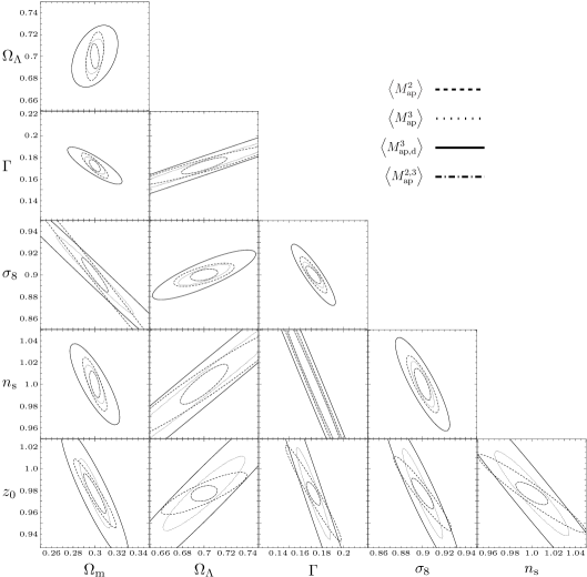
Figure 10: 1-$\sigma$-error ellipses from the Fisher matrix. The hidden parameters are kept fixed. Dashed line: $\langle M_{\rm ap}^{2}\rangle$, dotted line: $\langle M_{\rm ap}^{3}\rangle$, solid line: $\langle{M_{\rm ap,d}^{3}}\rangle$, dash-dotted line: combination of $\langle M_{\rm ap}^{2}\rangle$ and $\langle M_{\rm ap}^{3}\rangle$ as described in Sect. 5.1. If one of the parameters is $\Omega_{\rm m}$, a flat Universe is assumed (except for the $\Omega_{\rm m}$-$\Omega_{\Lambda}$-plot). The assumed survey area is 29 square degree.

5.3.2 Three and more parameters

We calculate the MVBs for three and more parameters simultaneously for various combinations of parameters and for each input data as described in Sect. 5.1. The results are given in Table 3. All hidden parameters are fixed to their fiducial values, see Table 1. If not both $\Omega_{\rm m}$ and $\Omega_{\Lambda}$ vary, a flat Universe is assumed.

In most of the cases, the error bars from the generalized third-order aperture mass statistics $\langle M_{\rm ap}^{3}\rangle$ are smaller than those from its second-order counterpart $\langle M_{\rm ap}^{2}\rangle$. This trend gets stronger the more free cosmological parameters are involved, since the measurement of $\langle M_{\rm ap}^{3}\rangle$ provides more data points and therefore more degrees of freedom. The skewness of the aperture mass $\langle M_{\rm ap,d}^{3}\rangle$ yields by far the worst constraints on the parameters.

In all of the cases, the combination of $\langle M_{\rm ap}^{2}\rangle$ and $\langle M_{\rm ap}^{3}\rangle$ results in an improvement on the parameter constraints. This improvement can be rather small, e.g. in the cases when both $\Gamma$ and $n_{\rm s}$ are involved. Then the combined MVB is dominated mainly by the MVB of $\langle M_{\rm ap}^{3}\rangle$, and the additional information from $\langle M_{\rm ap}^{2}\rangle$ is unimportant. However, for a number of parameter combinations, the combined error represents an improvement of a factor two and more, indicating that the dependence of the two statistics on the cosmological parameters is different to some degree, and their combination lifts the degeneracy substantially. Amongst other, this occurs for the pair $\Omega_{\rm m}$ and $\sigma_{8}$. Even if a rather good constraint on these two parameters from $\langle M_{\rm ap}^{3}\rangle$ is combined with a large MVB, the combined error can be reduced by a factor of two and more, thus the most prominent parameter degeneracy for second-order cosmic shear between $\Omega_{\rm m}$ and $\sigma_{8}$ can partially be broken by adding third-order statistics.

When $\langle M_{\rm ap}^{2}\rangle$ is combined with the generalized aperture-mass statistics (the case ‘2+3’) and the skewness (‘2+3d’), the first combination always yields better parameter constraints than the latter. For three free parameters, the first combination is typically a factor of two better, if more parameters are involved, the improvement factor is even larger, up to a factor of ten when all six parameters are free. Thus, the preference of $\langle M_{\rm ap}^{3}\rangle$ over the skewness of ${M_{\rm ap}}$ is justified also when it is combined with the second-order aperture mass statistics.

In general, constraints on the cosmological constant $\Omega_{\Lambda}$ are weaker than for the other parameters, and although the combination of second- and third order aperture mass statistics gives some improvement on the error, $\Omega_{\Lambda}$ remains the least known parameter.

Table 3: MVBs for various combinations of three and more cosmological parameters, corresponding to a 29 square degree survey. The hidden parameters are kept fixed. ‘2’, ‘3’, ‘3d’, ‘2+3d’ and ‘2+3’ stand for the five different input data as described in Sect. 5.1. If $\Omega_{\Lambda}$ is not a free parameter, a flat Universe is assumed.

	$\Omega_{\rm m}$	$\Omega_{\Lambda}$	$\Gamma$	$\sigma_{8}$	$n_{\rm s}$	$z_{0}$
2	0.077			0.104		0.035
3	0.041			0.053		0.047
3d	0.189			0.219		0.116
2+3d	0.027			0.030		0.029
2+3	0.016			0.016		0.019
2	0.087		0.015	0.119
3	0.063		0.017	0.078
3d	0.267		0.043	0.300
2+3d	0.027		0.012	0.044
2+3	0.015		0.008	0.024
2	0.083			0.110	0.029
3	0.059			0.072	0.035
3d	0.222			0.242	0.077
2+3d	0.026			0.040	0.025
2+3	0.014			0.022	0.017
2	0.017		0.093		0.200
3	0.010		0.051		0.113
3d	0.343		0.158		0.347
2+3d	0.010		0.063		0.138
2+3	0.005		0.035		0.078
2	0.087	0.106		0.113
3	0.057	0.089		0.067
3d	0.244	0.328		0.263
2+3d	0.033	0.056		0.047
2+3	0.019	0.037		0.028
2	0.095	0.744	0.353	0.285
3	0.065	0.117	0.053	0.085
3d	0.387	0.817	0.490	0.542
2+3d	0.066	0.243	0.078	0.053
2+3	0.028	0.088	0.026	0.030
2	0.569		0.270	0.552		0.645
3	0.080		0.033	0.088		0.091
3d	1.113		0.498	1.084		1.332
2+3d	0.218		0.090	0.224		0.213
2+3	0.069		0.031	0.072		0.069
2	0.674	2.447	2.199	1.857	1.618
3	0.065	0.127	0.065	0.085	0.125
3d	7.306	1.349	7.613	9.686	8.344
2+3d	0.075	0.263	0.101	0.070	0.186
2+3	0.031	0.094	0.043	0.034	0.090
2	3.554	5.535	2.677	3.719	2.169	3.553
3	0.110	0.328	0.084	0.092	0.140	0.220
3d	7.532	23.48	11.87	10.43	13.15	17.83
2+3d	0.928	1.101	0.620	0.996	0.701	0.812
2+3	0.079	0.124	0.050	0.080	0.090	0.072

5.4 Correlation between parameters

The correlation coefficient of the inverse Fisher matrix

$$r_{ij}=\frac{F^{-1}_{ij}}{\sqrt{F^{-1}_{ii}F^{-1}_{jj}}}$$ (22)

is a measure of the correlation between the $i^{\rm th}$ and $j^{\rm th}$ parameter. For $i\neq j$, it can vary between -1 and 1. In the two-dimensional case, $r_{12}=r_{21}=0$ corresponds to an error ellipse with major and minor axes parallel to the coordinate (parameter) axes – the probability distribution of the parameters factorizes. For $r_{12}\rightarrow 1$, the ellipse degenerates to a line.

Table 4 shows the correlation coefficient between all cosmological parameters considered in this work. For the combination of $\langle M_{\rm ap}^{2}\rangle$ and $\langle M_{\rm ap,d}^{3}\rangle$ (‘2+3d’), the correlation is very large for all parameter pairs, the difference to unity in some cases is only of the order of $10^{-3}$. The degeneracy directions of $\langle M_{\rm ap}^{2}\rangle$ and $\langle M_{\rm ap,d}^{3}\rangle$ are very similar, thus the combination of the two causes the correlation between parameters to be very high.

Table 4: The correlation coefficient $r_{ij}$ (22) of the inverse Fisher matrix (22). ‘2’, ‘3’, ‘3d’, ‘2+3d’ and ‘2+3’ stand for the five different input data as described in Sect. 5.1. Note that the correlation matrix $r$ is symmetric and unity on the diagonal.

		$\Omega_{\Lambda}$	$\Gamma$	$\sigma_{8}$	$n_{\rm s}$	$z_{0}$
	$\Omega_{\rm m}$	$-$0.80	0.71	$-$0.94	$-$0.79	$-$0.98
	$\Omega_{\Lambda}$		$-$0.15	0.56	0.28	0.90
	$\Gamma$			$-$0.90	$-$0.98	$-$0.57
2	$\sigma_{8}$				0.95	0.87
	$n_{\rm s}$					0.67
	$\Omega_{\rm m}$	$-$0.81	$-$0.31	$-$0.84	0.35	$-$0.81
	$\Omega_{\Lambda}$		0.66	0.41	$-$0.29	0.92
	$\Gamma$			$-$0.15	$-$0.69	0.63
3	$\sigma_{8}$				$-$0.14	0.38
	$n_{\rm s}$					$-$0.46
	$\Omega_{\rm m}$	$-$0.29	0.43	$-$0.81	$-$0.43	$-$0.24
	$\Omega_{\Lambda}$		0.74	$-$0.33	$-$0.74	1.00
	$\Gamma$			$-$0.88	$-$1.00	0.77
3d	$\sigma_{8}$				0.87	$-$0.37
	$n_{\rm s}$					$-$0.77
	$\Omega_{\rm m}$	$-$0.99	0.98	$-$1.00	$-$0.97	$-$1.00
	$\Omega_{\Lambda}$		$-$0.94	0.98	0.96	0.97
	$\Gamma$			$-$0.99	$-$0.98	$-$0.99
2+3d	$\sigma_{8}$				0.97	1.00
	$n_{\rm s}$					0.96
	$\Omega_{\rm m}$	$-$0.87	0.46	$-$0.99	$-$0.12	$-$0.92
	$\Omega_{\Lambda}$		$-$0.20	0.83	0.24	0.65
	$\Gamma$			$-$0.55	$-$0.66	$-$0.52
2+3	$\sigma_{8}$				0.17	0.90
	$n_{\rm s}$					$-$0.04

5.5 Stability

In order to check our Fisher matrix analysis for consistency and stability towards small changes of the input data, we redo our calculations with slightly different aperture radii. For changes of a couple of percent in the aperture radii, the resulting Fisher matrix elements vary of the order of up to 10 percent. The MVBs (see Sect. 5.2) fluctuate by about the same amount if two or three parameters are considered to be determined from the data simultaneously. However, for four and five free parameters, the MVBs are less stable, since the Fisher matrix is numerically very ill-conditioned and the inversion is a non-linear operation. In general, the MVBs for $\langle M_{\rm ap}^{3}\rangle$ are less stable than the ones for $\langle M_{\rm ap}^{2}\rangle$.

The eigenvectors of $F_{ij}^{-1}$ are less affected by a different sampling of aperture radius. Angles between original and modified eigenvectors are typically only a few degree. The variation of the correlation coefficient $r_{ij}$ (22) is less than $\sim 0.1$ if up to four parameters are considered. For a higher-dimensional Fisher matrix however, the variation can be higher, similar to the case of the MVB.

6 Summary and Conclusion

The power spectrum of large-scale (dark-)matter fluctuations was until recently the most important quantity that has been measured – directly or indirectly – by cosmic shear. Interesting constraints on cosmological parameters like $\Omega_{\rm m}$ and $\sigma_{8}$ have been obtained from second-order cosmic shear statistics.

The bispectrum of density fluctuations contains complementary information about structure evolution and cosmology. It is a measure of the non-Gaussianity of the large-scale structure. Current cosmic shear surveys are at the detection limit of measuring a non-Gaussian signal significantly, and future observations will certainly determine the bispectrum with high accuracy.

Combined measurements of the power and the bispectrum yield additional constraints on cosmological parameters and partially lift degeneracies between them. The second- and generalized third-order aperture mass statistics are local measures of the power and bispectrum, respectively. In this work, we made predictions about cosmological parameter estimations from combined measurements of these two weak lensing statistics. Using $\Lambda$CDM ray-tracing simulations, we calculated the covariance of $M_{\rm ap}^{2}$ and $M_{\rm ap}^{3}$ and their cross-correlation. We performed an extensive Fisher matrix analysis and obtained minimum variance bounds (MBVs) for a variety of combinations of cosmological parameters.

The generalized third-order aperture mass statistics (Schneider et al. 2004) is the correlator of ${M_{\rm ap}}$ for three different aperture radii. In contrast to the skewness of ${M_{\rm ap}}$ which probes the bispectrum for equilateral triangles only, the generalized third-order aperture mass is in principle sensitive to the bispectrum on the complete $\ell$-space. Therefore, it contains much more information about cosmology than the skewness alone.

The direction of degeneracy between the cosmological parameters considered here are similar for second- and third-order statistics. However, in most cases the combination of $\langle M_{\rm ap}^{2}\rangle$ and $\langle M_{\rm ap}^{3}\rangle$ gives substantial improvement on the predicted parameter constraints. The MVBs decrease by a factor of two or more for most of the parameter combinations. When the source redshift $z_{0}$ is not fixed but also to be determined from the data, the errors on the other parameters increase and the improvement by combining $\langle M_{\rm ap}^{2}\rangle$ and $\langle M_{\rm ap}^{3}\rangle$ is lowered.

We combined the second-order aperture mass statistics $\langle M_{\rm ap}^{2}\rangle$ with both the skewness and the generalized third-order aperture mass. The latter combination gives much better parameter constraints than the first one. For six parameters to be determined from the data simultaneously, the corresponding MVBs are better by a factor of about 10 for each parameter.

The $\Omega_{\rm m}$-$\sigma_{8}$-degeneracy is very prominent for both the second- and the third-order statistics of ${M_{\rm ap}}$ individually. However, by combining the two, the degeneracy is partially lifted – the 1-$\sigma$-errors of both parameters drop by a factor of two or more, depending on which other parameters are also considered to be determined from the data. The $n_{\rm s}$-$\Gamma$-degeneracy, however, can not be broken by combining $\langle M_{\rm ap}^{2}\rangle$ and $\langle M_{\rm ap}^{3}\rangle$, the determination of this pair of parameters is dominated by $\langle M_{\rm ap}^{3}\rangle$.

For the given range of 1 to 15 arc minutes for the aperture radii considered in this work the generalized third-order aperture mass statistics is dominant for the determination of most of the cosmological parameter combinations. The measurement error from $\langle M_{\rm ap}^{2}\rangle$ is in general larger than the one from $\langle M_{\rm ap}^{3}\rangle$. However, in most of the cases, even a weak constraint from $\langle M_{\rm ap}^{2}\rangle$ alone contributes valuable information to the combination of the two statistics, and the combined error is much smaller than the one from the individual measurements.

If the range of apertures is extended, would we expect the resulting improvement on the parameter estimation from the third-order aperture mass statistics to be higher than from second-order? For the former, the number of data points increases with the third power of the number of aperture radii, whereas for the latter, the increase is only linear. Thus, for an increase in the number of measured apertures, the constraints using $\langle M_{\rm ap}^{3}\rangle$ should improve more than those from $\langle M_{\rm ap}^{2}\rangle$. On the other hand, the data points are not at all uncorrelated; in fact, as it is shown in this work (Sect. 4.4), the correlation can be very strong for various combinations of aperture radius triples. Moreover, for large scales ($\theta\begin{array}[]{c}>\\ \sim\end{array}30^{\prime}$, see Fig. 2), the linear regime of the large-scale structure is probed, where non-Gaussian contributions are small, and the information content of third-order shear statistics is diminished. We conclude that angular scales up to about 30 arc minutes will be a good choice for the measurement of the generalized third-order aperture mass statistics of cosmic shear. The combination of this statistics with $\langle M_{\rm ap}^{2}\rangle$ will improve the resulting constraints on cosmological parameters quite substantially.

Appendix A Covariance of $M_{\rm ap}^{3}$ for shot-noise only

Analogous to Schneider et al. (2002), we analytically calculate the variance of $M_{\rm ap}^{3}$ in the case of shot-noise only, by integrating over the covariance of the shear 3PCF. An unbiased estimator of the natural component $\Gamma^{(0)}$ of the 3PCF (Schneider & Lombardi 2003) is

$$\hat{\Gamma}^{(0)}(T_{x})=\frac{1}{N_{\rm T}(T_{x})}\sum_{ijk}{\cal E}(ijk)\Delta_{T_{x}}(ijk),$$ (23)

where $T_{x}$ represents a triangle of points $\@vec{\vartheta}_{i},\@vec{\vartheta}_{j}$ and $\@vec{\vartheta}_{k}$, uniquely given e.g. by two side lengths $x_{1},x_{2}$ and the angle $\varphi$ between them. $N_{\rm T}(T_{x})$ is the number of triangles within the bin containing $T_{x}$, and ${\cal E}(ijk)$ an estimator of $\Gamma^{(0)}$; it is the following linear combination of products of ellipticities of three galaxies at positions $\@vec{\vartheta}_{i},\@vec{\vartheta}_{j}$ and $\@vec{\vartheta}_{k}$, i.e.

$${\cal E} = (\varepsilon_{\rm ttt}-\varepsilon_{{\rm t}\times\times}-\varepsilon_{\times{\rm t}\times}-\varepsilon_{\times\times{\rm t}})+$$ (24)

$${\rm i}(\varepsilon_{{\rm tt}\times}+\varepsilon_{{\rm t}\times{\rm t}}+\varepsilon_{\times{\rm tt}}-\varepsilon_{\times\times\times}),$$

where $\varepsilon_{\mu\nu\lambda}=\varepsilon_{\mu\nu\lambda}(\@vec{\vartheta}_{i},\@vec{\vartheta}_{j},\@vec{\vartheta}_{k})=\varepsilon_{\mu}(\@vec{\vartheta}_{i})\varepsilon_{\nu}(\@vec{\vartheta}_{j})\varepsilon_{\lambda}(\@vec{\vartheta}_{j})$ for $\mu,\nu,\lambda\in\{$‘${\rm t}$’,‘$\times$’$\}$, see eqs. (2) and (19) in Schneider & Lombardi (2003). The summation in (23) is performed over all possible triples of points $(\@vec{\vartheta}_{i},\@vec{\vartheta}_{j},\@vec{\vartheta}_{k})$, $\Delta_{T_{x}}(ijk)$ is unity if the triangle given by $(\@vec{\vartheta}_{i},\@vec{\vartheta}_{j},\@vec{\vartheta}_{k})$ is in the same bin as $T_{x}$, and zero otherwise.

The covariance of $\hat{\Gamma}^{(0)}$ consists of four terms, which are proportional to $\sigma_{\varepsilon}^{6}$, $\sigma_{\varepsilon}^{4}$, $\sigma_{\varepsilon}^{2}$ and $\sigma_{\varepsilon}^{0}$, respectively. In the case of vanishing cosmic variance, only the first term contributes; it reads

$${\rm Cov}(\hat{\Gamma}^{(0)},\hat{\Gamma}^{(0)};T_{x},T_{y})=\frac{1}{N_{\rm T}(T_{x})N_{\rm T}(T_{y})}$$ (25)

$$\times\sum_{ijklmn}\left\langle{\cal E}^{(\rm s)}(ijk){\cal E}^{(\rm s)*}(lmn)\right\rangle\Delta_{T_{x}}(ijk)\Delta_{T_{y}}(lmn),$$

where the superscript ‘s’ indicates the intrinsic (‘source’) ellipticity.

The term in angular brackets is non-zero only if the two triangles given by $(\@vec{\vartheta}_{i},\@vec{\vartheta}_{j},\@vec{\vartheta}_{k})$ and $(\@vec{\vartheta}_{l},\@vec{\vartheta}_{m},\@vec{\vartheta}_{n})$ are identical (under the assumption that different galaxies are intrinsically uncorrelated), and factorizes into a sum of products of three two-point terms, each of the form $\langle\varepsilon_{\mu}(\@vec{\vartheta}_{i})\varepsilon_{\mu^{\prime}}(\@vec{\vartheta}_{l})\rangle\delta_{il}\delta_{\mu\mu^{\prime}}$. With $\langle\varepsilon_{\rm t}\varepsilon_{\rm t}\rangle=\langle\varepsilon_{\times}\varepsilon_{\times}\rangle=\sigma_{\varepsilon}^{2}/2$ and $\langle\varepsilon_{\rm t}\varepsilon_{\times}\rangle=0$, the term in angular brackets becomes $8\cdot[\sigma_{\varepsilon}^{2}/2]^{3}=\sigma_{\varepsilon}^{6}$. The sum reduces to a triple sum over $\Delta_{T_{x}}(ijk)$ which is just the number of triangles in the respective bin. Finally, we get

$${\rm Cov}(\hat{\Gamma}^{(0)},\hat{\Gamma}^{(0)};T_{x},T_{y})=\frac{\sigma_{\varepsilon}^{6}}{N_{\rm T}(T_{x})}\bar{\delta}(T_{x},T_{y}),$$ (26)

where $\bar{\delta}(T_{x},T_{y})$ is zero if the two triangles $T_{x}$ and $T_{y}$ are in different bins, and unity otherwise.

The covariance of $M_{\rm ap}^{3}$ is obtained by integrating over the covariance of the 3PCF. This can be done analytically for the case when all six aperture radii are equal (this corresponds to the variance of $M_{\rm ap,d}^{3}$) and in the absence of a B-mode. We write eq. (62) of Schneider et al. (2004) in the following way, abbreviating the integral kernel with $R_{\theta}$,

$$\left\langle M^{3}_{\rm ap}(\theta_{1},\theta_{2},\theta_{3})\right\rangle=\int{\mathrm{d}}y_{1}\int{\mathrm{d}}y_{2}\int{\mathrm{d}}\psi$$ (27)

$$\times\tilde{\Gamma}^{(0)}_{\rm cen}(y_{1},y_{2},\psi)R_{\theta}(y_{1},y_{2},\psi).$$

where $\tilde{\Gamma}^{(0)}_{\rm cen}$ denotes the 3PCF in the center-of-mass projection, expressed as a function of triangle sides as described in Schneider et al. (2004).

Before we proceed, we note that for any function $f$,

$$\int{\mathrm{d}}y_{1}\int{\mathrm{d}}y_{2}\int{\mathrm{d}}\psi f(y_{1},y_{2},\psi)\bar{\delta}(T_{x},T_{y})$$ (28)

$$=f(x_{1},x_{2},\varphi)\Delta x_{1}\Delta x_{2}\Delta\varphi,$$

where $\Delta x_{1}$, $\Delta x_{2}$, $\Delta\varphi$ are given by the bin size in which the triangle $T_{x}$ is situated.

For simplicity, we assume that boundary effects due to the finite field size can be neglected. Then the number of triangles within the bin characterized by $(x_{1},x_{2},\varphi)$ is $N_{\rm T}(T_{x})=N\cdot(2\pi x_{2}\Delta x_{2}\,n)\cdot(\Delta x_{1}\Delta\varphi\,n)=2\pi An^{3}x_{1}\Delta x_{1}x_{2}\Delta x_{2}\Delta\varphi$, where $N$ is the total number of galaxies and $n$ is the galaxy density ($n=N/A$ for $A$ being the survey area). Thus,

$${\rm var}(M_{\rm ap,d}^{3};\theta)=\frac{\sigma_{\varepsilon}^{6}}{2\pi An^{3}}\int\frac{{\mathrm{d}}x_{1}}{x_{1}}\int\frac{{\mathrm{d}}x_{2}}{x_{2}}\int{\mathrm{d}}\varphi\,R^{2}_{\theta}(x_{1},x_{2},\varphi).$$ (29)

Solving the integral, we get

$${\rm var}(M_{\rm ap,d}^{3};\theta)=\frac{11}{15552\,\pi^{2}}\frac{\sigma_{\varepsilon}^{6}}{An^{3}\,\theta^{4}}=10^{-16}\left(\frac{\sigma_{\varepsilon}}{0.3}\right)^{6}$$ (30)

$$\times\left(\frac{A}{9\,{\rm deg}^{2}}\right)^{-1}\left(\frac{n}{25\,{\rm arcmin}^{-2}}\right)^{-3}\left(\frac{\theta}{\rm 1arcmin}\right)^{-4}.$$

Note that the variance of $M_{\rm ap}^{2}$ (Schneider et al. 2002) has the same dependence on the observed area $A$, but is only quadratically invsere as a function of both $n$ and $\theta$.

References

- Bernardeau et al. (2002) Bernardeau, F., Mellier, Y., & van Waerbeke, L. 2002, A&A, 389, L28
- Bernardeau et al. (1997) Bernardeau, F., van Waerbeke, L., & Mellier, Y. 1997, A&A, 322, 1
- Cooray & Sheth (2002) Cooray, A. & Sheth, R. 2002, Phys. Rep., 372, 1
- Crittenden et al. (2002) Crittenden, R. G., Natarajan, P., Pen, U.-L., & Theuns, T. 2002, ApJ, 568, 20
- Hamana et al. (2003) Hamana, T., Miyazaki, S., Shimasaku, K., et al. 2003, ApJ, 597, 98
- Hoekstra et al. (2002) Hoekstra, H., Yee, H. K. C., & Gladders, M. D. 2002, ApJ, 577, 595
- Jarvis et al. (2003) Jarvis, M., Bernstein, G., Fischer, P., & Smith, D. 2003, AJ, 125, 1014
- Jarvis et al. (2004) Jarvis, M., Bernstein, G., & Jain, B. 2004, MNRAS, 352, 338
- Kaiser et al. (1994) Kaiser, N., Squires, G., Fahlman, G., & Woods, D. 1994, in Clusters of galaxies, Proceedings of the XIVth Moriond Astrophysics Meeting, Méribel, France, 269, also astro-ph/9407004
- Kendall & Stuart (1969) Kendall, M. G. & Stuart, A. 1969, The Advanced Theory of Statistics, Vol. II (London: Griffin)
- Kilbinger & Schneider (2004) Kilbinger, M. & Schneider, P. 2004, A&A, 413, 465, Also astro-ph/0308119
- Ménard et al. (2003) Ménard, B., Hamana, T., Bartelmann, M., & Yoshida, N. 2003, A&A, 403, 817
- Peacock & Dodds (1996) Peacock, J. A. & Dodds, S. J. 1996, MNRAS, 280, L19
- Pen et al. (2003) Pen, U., Zhang, T., van Waerbeke, L., et al. 2003, ApJ, 592, 664
- Press et al. (1992) Press, W. H., Teukolsky, S. A., Flannery, B. P., & Vetterling, W. T. 1992, Numerical Recipes in C (Cambridge University Press)
- Schneider (1996) Schneider, P. 1996, MNRAS, 283, 837
- Schneider (2003) Schneider, P. 2003, A&A, 408, 829
- Schneider et al. (2004) Schneider, P., Kilbinger, M., & Lombardi, M. 2004, A&A, 431, 9
- Schneider & Lombardi (2003) Schneider, P. & Lombardi, M. 2003, A&A, 397, 809
- Schneider et al. (1998) Schneider, P., van Waerbeke, L., Jain, B., & Kruse, G. 1998, MNRAS, 296, 873
- Schneider et al. (2002) Schneider, P., van Waerbeke, L., Kilbinger, M., & Mellier, Y. 2002, A&A, 396, 1
- Schneider et al. (2002) Schneider, P., van Waerbeke, L., & Mellier, Y. 2002, A&A, 389, 729
- Scoccimarro & Couchman (2001) Scoccimarro, R. & Couchman, H. M. P. 2001, MNRAS, 325, 1312
- Smith et al. (2003) Smith, R. E., Peacock, J. A., Jenkins, A., et al. 2003, MNRAS, 341, 1311
- Spergel et al. (2003) Spergel, D. N., Verde, L., Peiris, H. V., et al. 2003, ApJS, 148, 175
- Sugiyama (1995) Sugiyama, N. 1995, ApJS, 100, 281
- Takada & Jain (2003) Takada, M. & Jain, B. 2003, ApJ, 583, L49
- Takada & Jain (2004) —. 2004, MNRAS, 348, 897
- Tegmark et al. (1997) Tegmark, M., Taylor, A., & Heavens, A. 1997, ApJ, 480, 22
- van Waerbeke (2000) van Waerbeke, L. 2000, MNRAS, 313, 524
- van Waerbeke et al. (1999) van Waerbeke, L., Bernardeau, F., & Mellier, Y. 1999, A&A, 342, 15
- van Waerbeke et al. (2005) van Waerbeke, L., Mellier, Y., & Hoekstra, H. 2005, A&A, 429, 75
- Zaldarriaga & Scoccimarro (2003) Zaldarriaga, M. & Scoccimarro, R. 2003, ApJ, 584, 559