MHD Turbulence: Properties of Alfven, Slow and Fast Modes

Abstract

We summarise basic properties of MHD turbulence. First, MHD turbulence is not so messy as it is believed. In fact, the notion of strong non-linear coupling of compressible and incompressible motions along MHD cascade is not tenable. Alfven, slow and fast modes of MHD turbulence follow their own cascades and exhibit degrees of anisotropy consistent with theoretical expectations. Second, the fast decay of turbulence is not related to the compressibility of fluid. Rates of decay of compressible and incompressible motions are very similar. Third, the properties of Alfven and slow modes are similar to their counterparts in the incompressible MHD. The properties of fast modes are similar to accoustic turbulence, which does require more studies. Fourth, the density at low Mach numbers and logarithm of density at higher Mach numbers exhibit Kolmogorov-type spectrum.

1 What is MHD Turbulence?

A fluid of viscosity $\nu$ becomes turbulent when the rate of viscous dissipation, which is $\sim\nu/L^{2}$ at the energy injection scale $L$, is much smaller than the energy transfer rate $\sim V_{L}/L$, where $V_{L}$ is the velocity dispersion at the scale $L$. The ratio of the two rates is the Reynolds number $Re=V_{L}L/\nu$. In general, when $Re$ is larger than $10-100$ the system becomes turbulent. Chaotic structures develop gradually as $Re$ increases, and those with $Re\sim 10^{3}$ are appreciably less chaotic than those with $Re\sim 10^{8}$. Observed features such as star forming clouds are very chaotic for $Re>10^{8}$. This makes it difficult to simulate realistic turbulence. The currently available 3D simulations containing 512 grid cells along each side can have $Re$ up to $\sim O(10^{3})$ and are limited by their grid sizes. Therefore, it is essential to find “scaling laws” in order to extrapolate numerical calculations ($Re\sim O(10^{3})$) to real astrophysical fluids ($Re>10^{8}$). We show below that even with its limited resolution, numerics is a great tool for testing scaling laws.

Kolmogorov theory provides a scaling law for incompressible non-magnetized hydrodynamic turbulence (Kolmogorov 1941). This law provides a statistical relation between the relative velocity $v_{l}$ of fluid elements and their separation $l$, namely, $v_{l}\sim l^{1/3}$. An equivalent description is to express spectrum $E(k)$ as a function of wave number $k$ ($\sim 1/l$). The two descriptions are related by $kE(k)\sim v_{l}^{2}$. The famous Kolmogorov spectrum is $E(k)\sim k^{-5/3}$. The applications of Kolmogorov theory range from engineering research to meteorology (see Monin & Yaglom 1975) but its astrophysical applications are poorly justified and the application of the Kolmogorov theory can lead to erroneous conclusions (see reviews by Lazarian et al. 2003 and Lazarian & Yan 2003).

Let us consider incompressible MHD turbulence first. There have long been understanding that the MHD turbulence is anisotropic (e.g. Shebalin et al. 1983). Substantial progress has been achieved recently by Goldreich & Sridhar (1995; hereafter GS95), who made an ingenious prediction regarding relative motions parallel and perpendicular to magnetic field B for incompressible MHD turbulence. An important observation that leads to understanding of the GS95 scaling is that magnetic field cannot prevent mixing motions of magnetic field lines if the motions are perpendicular to the magnetic field. Those motions will cause, however, waves that will propagate along magnetic field lines. If that is the case, the time scale of the wave-like motions along the field, i.e. $\sim l_{\|}/V_{A}$, ($l_{\|}$ is the characteristic size of the perturbation along the magnetic field and $V_{A}=B/\sqrt{4\pi\rho}$ is the local Alfven speed) will be equal to the hydrodynamic time-scale, $l_{\perp}/v_{l}$, where $l_{\perp}$ is the characteristic size of the perturbation perpendicular to the magnetic field. The mixing motions are hydrodynamic-like. They obey Kolmogorov scaling, $v_{l}\propto l_{\perp}^{1/3}$, because incompressible turbulence is assumed. Combining the two relations above we can get the GS95 anisotropy, $l_{\|}\propto l_{\perp}^{2/3}$ (or $k_{\|}\propto k_{\perp}^{2/3}$ in terms of wave-numbers). If we interpret $l_{\|}$ as the eddy size in the direction of the local magnetic field. and $l_{\perp}$ as that in the perpendicular directions, the relation implies that smaller eddies are more elongated. The latter is natural as it the energy in hydrodynamic motions decreases with the decrease of the scale. As the result it gets more and more difficult for feeble hydrodynamic motions to bend magnetic field lines.

GS95 predictions have been confirmed numerically (Cho & Vishniac 2000; Maron & Goldreich 2001; Cho, Lazarian & Vishniac 2002a, hereafter CLV02a; see also CLV03a); they are in good agreement with observed and inferred astrophysical spectra (see CLV03a). What happens in a compressible MHD? Does any part of GS95 model survives? Literature on the properties of compressible MHD is very rich (see reviews by Pouquet 1999; Cho & Lazarian 2003b and references therein). Higdon (1984) theoretically studied density fluctuations in the interstellar MHD turbulence. Matthaeus & Brown (1988) studied nearly incompressible MHD at low Mach number and Zank & Matthaeus (1993) extended it. In an important paper Matthaeus et al. (1996) numerically explored anisotropy of compressible MHD turbulence. However, those papers do not provide universal scalings of the GS95 type.

The complexity of the compressible magnetized turbulence with magnetic field made some researchers believe that the phenomenon is too complex to expect any universal scalings for molecular cloud research. Alleged high coupling of compressible and incompressible motions is often quoted to justify this point of view (see discussion of this point below).

In what follows we discuss the turbulence in the presence of regular magnetic field which is comparable to the fluctuating one. Therefore for most part of our discussion, we shall discuss results obtained for $\delta V\sim\delta B/\sqrt{4\pi\rho}\sim B_{0}/\sqrt{4\pi\rho}$, where $\delta B$ is the r.m.s. strength of the random magnetic field. However, we would argue that our choice is not so restrictive as it may be seen. Indeed, at the scales where the velocity perturbations are much larger than the Alfven velocity, the dynamical importance of magnetic field is small. Therefore we expect that at those scales turbulent motions are close to hydrodynamic ones. At smaller scales where the local turbulent velocity gets smaller than the Alfven speed we believe that our picture will be approximately true. We think that the local magnetic field should act as $B_{0}$, while the small scale perturbations happen in respect to that local field. This reasoning is in agreement with calculations in Cho, Lazarian & Vishniac (2003b) and Cho & Lazarian (2003a).

2 Does the Decay of MHD Turbulence Depend on Compressibility?

Many astrophysical problems, e.g. the turbulent support of molecular clouds (see review by McKee 1999), critically depends on the rate of turbulence decay. For a long time magnetic fields were thought to be the means of making turbulence less dissipative. Therefore it came as a surprise when numerical calculations by Mac Low et al. (1998) and Stone, Ostriker, & Gammie (1998) indicated that compressible MHD turbulence decays as fast as the hydrodynamic turbulence. This gives rise to a erroneous belief that it is the compressibility that is responsible for the rapid decay of MHD turbulence.

This point of view has been challenged in Cho & Lazarian (2002, 2003a, henceforth CL02 and CL03, respectively). In these papers a technique of separating different MHD modes was developed and used (see Fig. 1). This allowed us to follow how the energy was redistributed between these modes.

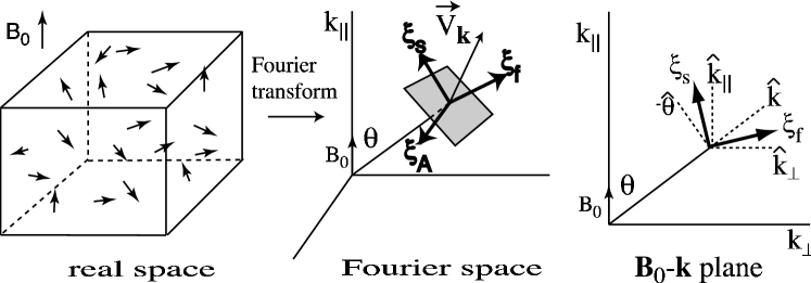
Figure 1: Separation method. We separate Alfven, slow, and fast modes in Fourier space by projecting the velocity Fourier component ${\bf v_{k}}$ onto bases ${\bf\xi}_{A}$, ${\bf\xi}_{s}$, and ${\bf\xi}_{f}$, respectively. Note that ${\bf\xi}_{A}=-\hat{\bf\varphi}$. Slow basis ${\bf\xi}_{s}$ and fast basis ${\bf\xi}_{f}$ lie in the plane defined by ${\bf B}_{0}$ and ${\bf k}$. Slow basis ${\bf\xi}_{s}$ lies between $-\hat{\bf\theta}$ and $\hat{\bf k}_{\|}$. Fast basis ${\bf\xi}_{f}$ lies between $\hat{\bf k}$ and $\hat{\bf k}_{\perp}$.

Should the different MHD modes be strongly coupled when the turbulence is strong? A naive answer is “yes”. Indeed, strong turbulence implies strong field line wondering. This mixes up Alfven and fast modes. In addition, one can show through calculations that the magnetic non-linearities result in the drainage of energy from Alfvenic cascade. However, a remarkable feature of the GS95 model is that Alfven perturbations cascade to small scales over just one wave period, which gets shorter and shorter as we move along the cascade. The competing effects coupling different modes usually require more time. We note that as the consequence of this reasoning we should assume that the properties of the Alfvenic cascade (incompressible cascade!) should not strongly depend on the sonic Mach number.

Are the arguments above correct? The generation of compressible motions (i.e. radial components in Fourier space) from Alfvenic turbulence is a measure of mode coupling. How much energy in compressible motions is drained from Alfvenic cascade? According to closure calculations (Bertoglio, Bataille, & Marion 2001; see also Zank & Matthaeus 1993), the energy in compressible modes in hydrodynamic turbulence scales as $\sim M_{s}^{2}$ if $M_{s}<1$. CL03 conjectured that this relation can be extended to MHD turbulence if, instead of $M_{s}^{2}$, we use $\sim(\delta V)_{A}^{2}/(a^{2}+V_{A}^{2})$. (Hereinafter, we define $V_{A}\equiv B_{0}/\sqrt{4\pi\rho}$, where $B_{0}$ is the mean magnetic field strength.) However, since the Alfven modes are anisotropic, this formula may require an additional factor. The compressible modes are generated inside the so-called Goldreich-Sridhar cone, which takes up $\sim(\delta V)_{A}/V_{A}$ of the wave vector space. The ratio of compressible to Alfvenic energy inside this cone is the ratio given above. If the generated fast modes become isotropic (see below), the diffusion or, “isotropization” of the fast wave energy in the wave vector space increase their energy by a factor of $\sim V_{A}/(\delta V)_{A}$. This results in

$$\frac{(\delta V)_{rad}^{2}}{(\delta V)_{A}^{2}}\sim\left[\frac{V_{A}^{2}+a^{2}}{(\delta V)^{2}_{A}}\frac{(\delta V)_{A}}{V_{A}}\right]^{-1},$$ (1)

where $(\delta V)_{rad}^{2}$ and $(\delta V)_{A}^{2}$ are energy of compressible and Alfven modes, respectively. Eq. (1) suggests that the drain of energy from Alfvenic modes is marginal along the cascade when the amplitudes of perturbations are weak. Results of calculations shown in Fig. 2 support the theoretical predictions.

We may summarize this issue in the following way. For the incompressible motions to decay fast, there is no requirement of coupling with compressible motions. The marginal coupling of the compressible and incompressible modes allows us to study these modes separately.

Figure 2: Mode coupling studies. (a)left: Square of the r.m.s. velocity of the compressible modes. We use $144^{3}$ grid points. Only Alfven modes are allowed as the initial condition. “Pluses” are for low $\beta$ cases ($0.02\leq\beta\leq 0.4$). “Diamonds” are for high $\beta$ cases ($1\leq\beta\leq 20$). (b)middle: Generation of fast modes. Snapshot is taken at t=0.06 from a simulation (with $144^{3}$ grid points) that started off with Alfven modes only. Initially, $\beta$ (ratio of gas to magnetic pressure, $P_{g}/P_{mag}$) $=0.2$ and $M_{s}$ (sonic Mach number) $\sim 1.6$. (c)right: Comparison of decay rates. Decay of Alfven modes is not much affected by other (slow and fast) modes. We use $216^{3}$ grid points. Initially, $\beta=0.02$ and $M_{s}\sim 4.5$ for the solid line and $M_{s}\sim 7$ for the dotted line. Note that initial data are, in some sense, identical for the solid and the dotted lines. The sonic Mach number for the solid line is smaller because we removed fast and slow modes from the initial data before the decay simulation. For the dotted line, we did not remove any modes from the initial data. From CL03.

3 What are the scalings for velocity and magnetic field?

Some hints about effects of compressibility can be inferred from the GS95 seminal paper. More discussion was presented in Lithwick & Goldreich (2001), which primary deals with electron density fluctuations in the regime of high $\beta$, i.e. ($\beta\equiv P_{gas}/P_{mag}\gg 1$). As the incompressible regime corresponds to $\beta\rightarrow\infty$, so it is natural to expect that for $\beta\gg 1$ the GS95 picture would persist. Lithwick & Goldreich (2001) also speculated that for low $\beta$ plasmas the GS95 scaling of slow modes may be applicable. A detailed study of compressible mode scalings is given in CL02 and CL03.

Our considerations above about the mode coupling can guide us in the discussion below. Indeed, if Alfven cascade evolves on its own, it is natural to assume that slow modes exhibit the GS95 scaling. Indeed, slow modes in gas pressure dominated environment (high $\beta$ plasmas) are similar to the pseudo-Alfven modes in incompressible regime (see GS95; Lithwick & Goldreich 2001). The latter modes do follow the GS95 scaling. In magnetic pressure dominated environments or low $\beta$ plasmas, slow modes are density perturbations propagating with the sound speed $a$ parallel to the mean magnetic field. Those perturbations are essentially static for $a\ll V_{A}$. Therefore Alfvenic turbulence is expected to mix density perturbations as if they were passive scalar. This also induces the GS95 spectrum.

The fast waves in low $\beta$ regime propagate at $V_{A}$ irrespectively of the magnetic field direction. In high $\beta$ regime, the properties of fast modes are similar, but the propagation speed is the sound speed $a$. Thus the mixing motions induced by Alfven waves should marginally affect the fast wave cascade. It is expected to be analogous to the acoustic wave cascade and hence be isotropic.

Results of numerical calculations from Cho & Lazarian (CL03, Cho & Lazarian 2004) for magnetically dominated media similar to that in molecular clouds are shown in Fig. 3. They support theoretical considerations above.

Figure 3: $M_{s}\sim 2.2$, $M_{A}\sim 0.7$, $\beta\sim 0.2$, and $216^{3}$ grid points. (a) Spectra of Alfvén modes follow a Kolmogorov-like power law. (b) Eddy shapes (contours of same second-order structure function, $SF_{2}$) for velocity of Alfvén modes shows anisotropy similar to the GS95 ($r_{\|}\propto r_{\perp}^{2/3}$ or $k_{\|}\propto k_{\perp}^{2/3}$). The structure functions are measured in directions perpendicular or parallel to the local mean magnetic field in real space. We obtain real-space velocity and magnetic fields by inverse Fourier transform of the projected fields. (c) Spectra of slow modes also follow a Kolmogorov-like power law. (d) Slow mode velocity shows anisotropy similar to the GS95. We obtain contours of equal $SF_{2}$ directly in real space without going through the projection method, assuming slow mode velocity is nearly parallel to local mean magnetic field in low $\beta$ plasmas. (e) Spectra of fast modes are compatible with the IK spectrum. (f) The magnetic $SF_{2}$ of fast modes shows isotropy. From CL02

Figure 4: left panel: Mach number is 0.35, central panel: Mach number is 7 (figures are from CL03), right panel: Mach number is 7, power spectra of: solid – density, crosses – velocity, triangles – logarithm of density, squares – density restricted from above by $2\rho_{0}$, short streak is a Kolmogorov scaling, $k^{-5/3}$.

4 What is the scaling of fast waves?

At both low and high $\beta$ fast magnetosonic waves have nearly isotropic dispersion relation, which makes them similar to simple acousic waves. In fact, the analytical dependence of the wave speed on the angle between ${\bf k}$ and ${\bf B}$ is the same for the values of $\alpha=c_{S}^{2}/V_{A}^{2}=\beta(\gamma/2)$ equal to $x$ or $1/x$. So the case of $\alpha=1$ represents most anisotropy possible. In the so called wave turbulence approach perturbations of physical quantities are represented as a combination of weakly interacting waves. (Zakharov, 1965; Zakharov, Sagdeev, 1970; Kats, Kontorovich, 1973)

In the leading order three wave processes waves obey conservation laws $\omega=\omega_{1}+\omega_{2}$, $\bf{k}={\bf k_{1}}+{\bf k_{2}}$. The form of resonant surfaces that came from solving above equations play crucial role in the nature of wave interactions. For a nondispersive acousic wave $\omega=ck$ and the resonance occurs only when all three ${\bf k}$ are collinear. It could be shown that despite the anisotropy, even for the case of $\alpha=1$ fast MHD waves can interact only along rays. In this sense both sound and fast waves are a special case in the theory of weak or wave turbulence.

The decomposition into interacting waves is conducted by the change to normal variables $a_{i}(k)$, $a_{i}^{*}(k)$, which are the classic versions of creation and annihilation operators, and leaving only quadratic and qubic terms of the power series of the Hamiltonian with respect to $a$ This method could not be questioned until the perturbation amplitudes are small, however, usually, wave turbulence approach takes another step of assuming the randomness of phases, which allows to write the the kinetic equation for the $\langle a_{k}a^{*}_{k}\rangle$, or the occupation numbers of the waves. The applicability of this approach is seriosly questioned in the case of nondispersive waves and collinear interaction, since waves, travelling in the same direction with the same speed have an infinite time to interact, hence their phases should reveal growing deviation from randomness. This is clearly demonstrated on the analythically solvable one-dimentional Burgers equation. In this case shocks are formed after finite time, even with arbitrarily small nonlinearity. Shocks could be described as a collection of waves with specific phases.

However the validity of the kinetic equation approach has been advocated recently in 3D in the framework of the generalized kinetic equation, in which waves are slightly damped (L’vov, et al. 2000). In the above paper slight defocusing of isotropisation of the distribution function reported and the damping is estimated from the nonlinear interaction itself.

The kinetic equation approach is thought to work much better in the case of dispersive waves, which allow for noncollinear three wave interactions. For example, if $\omega=k^{1+\epsilon}$, $\epsilon>0$, triangle inequality allows for such interactions, while for $\epsilon<0$ it doesn’t. It was shown (L’vov, Falkovich, 1981) that the above dispersion with $\epsilon>0$ lead to focusing, i.e. anisotropic part of the distribution increases faster with k than isotropic one. This effect could be understood from the simple physical picture of the resonantly interacting three waves with ${\bf k}$ being the sum of ${\bf k}_{1}$ and ${\bf k}_{2}$ and $k<k_{1}+k_{2}$. The angle between ${\bf k}_{1}$ and ${\bf k}_{2}$ is in most cases larger than the angle between ${\bf k}$ and ${\bf k}_{1}$ or ${\bf k}_{2}$.

Even in the case of dispersive waves the validity of kinetic equation approach has been questioned (see, e.g. Majda et al. 1997) in 1-dimensional case by numerical simulations. In this case various types of structures that violate the randomness of phase has been proposed (Zakharov, et al, 2004)

Self-similar solutions for several types of waves were constructed in the kinetic equation approach using Zakharov transformations in ${\bf k}$ space in the collisional integral. (Zakharov, 1965; Katz, Kontorovich, 1973). For the particular case of the acoustic wave turbulent 1D energy density was predicted to scale like $k^{-3/2}$.

5 What is the scaling of density?

Density at low Mach numbers follow the GS95 scaling when the driving is incompressible (CL03). However, CL03 showed that this scaling substantially changes for high Mach numbers. Fig. 4 shows that at high Mach numbers density fluctuations get isotropic. Moreover, our present studies confirm the CL03 finding that the spectrum of density gets substantially flatter than the GS95 one (see also Cho & Lazarian 2004). Note, that a model of random shocks would produce a spectrum steeper than the GS95 one.

The study of the density perturbation scaling properties and statistics regarless of the perturbation origin (slow or fast modes) in numerical simulations or observations could be a model-independent test for applicability of the incompressible MHD approach in small scales. Indeed, incompressible MHD requires divergent-free motions, and set the density constant everywhere. Flatter density spectrum has been reported in both low-beta MHD and purely hydrodynamic high Mach simulations.

In the highly compressible case we expect significant non-linear perturbations of density, but what the nature of these perturbations? In a compressible isothermal hydrodynamics equations are invariant under transformation $\rho\rightarrow C\rho$, it is, then, natural to consider $\log\rho$ so that equations have additive symmetry. If we expect the log-density buildup to be a random process, then a PDF of log-density will be gaussian. It was confirmed in high-Mach hydrodynamic 1D simulations. For the arbitrary polytropic equation of state $\gamma\not=1$ the PDF developed power-law tails on both sides. (Passot, Vazquez-Semadeni, 1998)

Our figure 4 confirmes that the flattening of the density spectra 3D simulations is due to very high density spikes, normally present in both MHD and purely hydrodynamic data. Indeed, both the spectra of log-density and the spectra of density, constrained from above by several $\rho_{0}$ do not have flattening, but bear good resemblance to the velocity spectra, and have scaling close to Kolmogorov. A simple removal of high density peaks also results in the Kolmogorov-type spectrum, which confirms the origin of peaks due to high density clupms produced by large scale driving.

It should be noted that this result holds true even in the case of relatively highly magnetized fluid, with $M_{A}$ of 0.5. It is natural to suggest then that a random buildup of log-density, which in magnetized case will be governed by slow mode and be essentially 1-dimensional, works as well in this case, even though MHD equations no longer posess the symmetry of $\log\rho\rightarrow\log\rho+C$.

The result that a highly compressible turbulence leaves the density field perturbed by 2-3 orders of magnitude, and even higher in small areas might undermine certain models of incompressible turbulent transport, that require weak interaction of waves making transport non-local.

6 Is MHD turbulence and Hydro turbulence similar?

Not only Kolmogorov scaling indicate the similarity between the hydro and MHD turbulence. Studies of higher order correlations when the motions perpendicular to the local magnetic field are considered show high degree of similarity between the magnetized and non-magnetized turbulence (CLV02b). This is suggestive that motions perpendicular to local magnetic field are essentially hydrodynamic. For some problems, e.g. turbulent heat transport (see Cho et al 2003), this entails similar results with and without ${\bf B}$.

Nevertheless, the most important difference between hydro and magnetic turbulence is the scale-dependent anisotropy of the latter. This peculiar type of anisotropy entails dramatic consequencies for the transport of cosmic rays or acceleration of charged dust (see Yan & Lazarian 2004 and references therein).

7 Summary

1. MHD turbulence is not a mess. The turbulent cascade consists of Alfven, slow and fast modes cascades. Fast modes follow accoustic turbulence cascade, while Alfven and slow modes are similar to their counterparts in incompressible MHD.

2. Fast decay of MHD turbulence is not due to strong coupling of compressible and incompressible motions. The transfer of energy from Alfven to compressible modes is small. The Alfven mode develops on its own and decays fast.

3. Density fluctuations follow the scaling of Alfvenic part of the cascade only at small Mach numbers. At large Mach numbers the log-density shows Kolmogorov spectrum.

AcknowledgmentsWe are grateful to Jungyeon Cho for data and nice discussion. We acknowledge NSF grant AST 0307869 and the NSF Center for Magnetic Self-Organization in the Laboratory and Astrophysical Plasmas.

References

- [1] Bell A.R., Lucek S.G., 2001, MNRAS 321, 433-438
- Bertoglio et al. (2001) Bertoglio J.-P., Bataille F., Marion J.-D., 2001, Phys. Fluids, 13, 290
- Boldyrev et al. (2002) Boldyrev S., Nordlund Å., Padoan P., 2002a, Phys. Rev. Lett. 89, 031102
- Cho & Lazarian (2002a) Cho J., Lazarian A., 2002a, Phy. Rev. Lett., 88, 245001 (CL02)
- (5) Cho J., Lazarian A., 2003a, MNRAS, 345, 325 (CL03)
- (6) Cho J., Lazarian A., 2003b, preprint (astro-ph/0301462)
- (7) Cho J., Lazarian A., 2004, preprint (astro-ph/0411031)
- Cho et al. (2003) Cho J., Lazarian A., Honein A., Knaepen B., Kassinos S., Moin P., 2003, ApJ, 589, L77
- Cho et al. (2002a) Cho J., Lazarian A., Vishniac E., 2002a, ApJ, 564, 291 (CLV02a)
- Cho et al. (2002b) Cho J., Lazarian A., Vishniac E., 2002b, ApJ, 566, L49 (CLV02b)
- Cho et al. (2003a) Cho J., Lazarian A., Vishniac E., 2003a, in Turbulence and Magnetic Fields in Astrophysics, eds. E. Falgarone, T. Passot (Springer LNP), p56 (astro-ph/0205286) (CLV03a)
- Cho et al. (2003b) Cho J., Lazarian A., Vishniac E., 2003b, ApJ, 595, 812
- Cho & Vishniac (2000b) Cho J., Vishniac E., 2000, ApJ, 539, 273
- (14) Cohen R.H, Kulsrud R.M., 1974, Phys. Fluids, 17, 12, 2219
- Del Zanna, Velli, & Londrillo (2001) Del Zanna L., Velli M., Londrillo P., 2001, A&A, 367, 705
- (16) Galtier S., Nazarenko S.V., Newell A.C., Pouquet A., 2000, J. Plasma Phys., 63(5), 447-488
- Goldreich & Sridhar (1995) Goldreich P., Sridhar S., 1995, ApJ, 438, 763 (GS95)
- (18) Goldstein M.L., 1978, Astrophys. J. 219, 700
- Higdon (1984) Higdon J. C., 1984, ApJ, 285, 109
- (20) Jayanti V., Hollweg J. V., 1993, J. Geophys. Res. 98, 13247
- (21) Kats A.V., Kontorovich V.M., 1973, Zh. Eksp. Teor. Fiz. 64, 153 [Sov. Phys. JETP 37, 80 (1973)]
- Kolmogorov (1941) Kolmogorov A., 1941, Dokl. Akad. Nauk SSSR, 31, 538
- Lazarian et al. (2003) Lazarian A., Petrosian V., Yan H., Cho J., 2003, in press (astro-ph/0301181)
- Lazarian, Vishniac & Cho (2003) Lazarian A., Vishniac E. T., Cho J., 2004, ApJ, 603, 180 (LVC04)
- Lazarian & Yan (2002) Lazarian A., Yan H., 2003, in “Astrophysical Dust” eds. A. Witt & B. Draine, APS, in press
- Lithwick & Goldreich (2001) Lithwick Y., Goldreich P., 2001, ApJ, 562, 279
- (27) L’vov V.S., Fal’kovich G.E., 1981, Zh. Eksp. Teor. Fiz. 80, 592 [Sov. Phys. JETP 53, 299]
- (28) L’vov V.S., L’vov Yu.V., Pomyalov A., 2000, Phys. Rev. E 61, 3, 2586
- (29) Mac Low M.-M., Klessen R., Burkert A., Smith M., 1998, Phys. Rev. Lett., 80, 2754
- (30) Majda A.J., McLaughlin D.W., Tabak E.G., 1997, J. Nonlin. Sci. 6, 9-44
- Maron & Goldreich (2001) Maron J., Goldreich P. 2001, ApJ, 554, 1175
- Matthaeus & Brown (1988) Matthaeus W. H., Brown M. R. 1988, Phys. Fluids, 31(12), 3634
- Matthaeus et al. (1996) Matthaeus W. H., Ghosh S., Oughton S., Roberts D. A., 1996, J. Geophysical Res., 101(A4), 7619
- (34) McKee C., 1999, The Origin of Stars and Planetary Systems. Eds. Charles J. Lada and Nikolaos D. Kylafis. Kluwer, p.29
- (35) Monin A.S., Yaglom A.M., 1975, Statistical Fluid Mechanics: Mechanics of Turbulence, vol. 2, The MIT Press
- (36) Nazarenko S.V., Newell A.C., Galtier S., 2001, Physica D 152-153 646-652
- (37) Nordlund A., Padoan P., 2003, in Turbulence and Magnetic Fields in Astrophysics, eds. E. Falgarone & T. Passot (Springer LNP), p.271
- (38) Passot T., Vázquez-Semadeni E., 1998, Phys. Rev. E 58(4), 4501-4510
- (39) Porter D., Pouquet A., Woodward P., 2002, Phys. Rev. E, 66, 026301
- (40) Pouquet A. 1999, in Interstellar Turbulence, p.87
- (41) Ptuskin V.S., Zirakashvili V.N., 2003, A&A, 403, 1
- Shebalin et al. (1983) Shebalin J. V., Matthaeus W. H., Montgomery D. C., 1983, J. Plasma Phys., 29, 525
- Stone, Ostriker, & Gammie (1998) Stone J., Ostriker E., Gammie C., 1998, ApJ, 508, L99
- (44) Vestuto J. G., Ostriker E. C., Stone, J. M., 2003, ApJ, 590, 858
- (45) Zakharov V.E., 1965, Prikl. Mekh. Teor. Fiz. 4, 35
- (46) Zakharov V., Dias F., Pushkarev A., 2004, Phys Rep. 398, 1-65
- (47) Zakharov V.E., Sagdeev R.Z., 1970, Dokl. Akad. Nauk SSSR 192, 297 [Soviet Phys.-Doklady 15, 439 (1970)]
- Zank & Matthaeus (1993) Zank G. P., Matthaeus W. H., 1993, Phys. Fluids A, 5(1), 257
- (49) Yan, H. & Lazarian, A. 2004, ApJ, 614, 757