Pulsars as Tools for Fundamental Physics & Astrophysics

Abstract

The sheer number of pulsars discovered by the SKA, in combination with the exceptional timing precision it can provide, will revolutionize the field of pulsar astrophysics. The SKA will provide a complete census of pulsars in both the Galaxy and in Galactic globular clusters that can be used to provide a detailed map of the electron density and magnetic fields, the dynamics of the systems, and their evolutionary histories. This complete census will provide examples of nearly every possible outcome of the evolution of massive stars, including the discovery of very exotic systems such as pulsar black-hole systems and sub-millisecond pulsars, if they exist. These exotic systems will allow unique tests of the strong field limit of relativistic gravity and the equation of state at extreme densities. Masses of pulsars and their binary companions — planets, white dwarfs, other neutron stars, and black holes — will be determined to $\sim 1$% for hundreds of objects. With the SKA we can discover and time highly-stable millisecond pulsars that comprise a pulsar-timing array for the detection of low-frequency gravitational waves. The SKA will also provide partial censuses of nearby galaxies through periodicity and single-pulse detections, yielding important information on the intergalactic medium.

1 Introduction

Neutron stars (NSs) are accessible to observation as pulsars and thus provide our only means for probing the most extreme states of matter in the present-day Universe, which in turn will enable a vast range of transforming science goals to be addressed, among which are

• Strong-field tests of gravity including the Cosmic Censorship Conjecture and the no-hair theorem of BHs.

• Detection of a cosmological gravitational wave background.

• Mapping the complete structure of the Milky Way and revealing properties of the Galactic Center.

• Probing the intergalactic medium in new ways.

• Identifying the equation-of-state of super-dense matter.

• Quantifying the roles of magnetic fields and turbulence in core-collapse physics.

• Understanding the superfluid interiors and relativistic magnetospheres of NS.

• Unraveling the evolutionary and dynamical histories and properties of all Galactic globular clusters.

• Discoveries of extrasolar planets.

Internal densities $\sim$ ten times nuclear density have not existed since the Universe was about 1 ms old. The actual state of matter in the core of a NS is presently not known. It may consist of de-confined quark matter or hyperonic matter produced in a phase transition that occurred during or shortly after the core collapse of the progenitor star. Intermediate regions of the NS consist of neutrons and trace protons in, respectively, superfluid and super-conducting states achieved after the NS cooled to about $10^{9}$ degrees. The outer regions include an $\sim 1$ km thick crust composed of iron-like nuclei surrounded by an ocean about 1 cm deep [66]. The magnetic field anchored to the crust and extending to interstellar space is sufficiently strong that it elongates the atoms comprising the crust. The surface gravity, about $10^{9}$ times that of the Earth’s, is the largest of any object in the Universe subject to observation, and corresponds to a gravitational redshift $\sim 0.3$.

While NS gravity is strong, radio pulsars and probably most NSs are even more extreme electromagnetically. By virtue of spin periods $P\sim 1$s and magnetic fields $B\sim 10^{8}-10^{14}$ Gauss, the electric force on a surface proton $\sim 10^{11}$ times larger than the gravitational force. Voltage drops $\sim 10^{12}$ volts across the magnetosphere accelerate particles that can radiate across the entire electromagnetic spectrum. This makes some pulsars visible in every astronomical window [76]. Most of what is to be learned from pulsars requires observations of their radio emission, often providing a unique source of information, and otherwise providing information that complements multiwavelength studies, particularly at high energies.

The feature that gives pulsars their name — pulsed radio emission — allows most NSs to be detected at levels well below the sky confusion limit and also provides the means for using pulsars as physics laboratories. Coherent radio emission is associated with the collimation of the flow of particles at the poles of the large-scale magnetic field in combination with relativistic beaming. The spin-driven sweep of the beam across the line of sight then provides the distinctive pulsation of the electromagnetic signal.

The suitability for using pulsars as clocks depends on the regularity by which the spin evolves with time. Spin noise in some objects, which evidently reflects activity within the crust and superfluid, is large enough to mask many of the physical effects of interest that provide only subtle timing signatures. However, spin noise itself, including rapid spinups (glitches), is itself valuable information on NS interiors. All pulsars are stable enough so that timing measurements can yield fundamental parameters such as the period vs. epoch, $P(t)$ and its time derivative $\dot{P}$, along with the dispersion measure DM. Objects with the narrowest pulses, the shortest periods, and the most stable rotation rates — millisecond pulsars — yield the greatest opportunities for exploring relativistic gravity. Extrinsic gravitational effects include perturbations of pulse arrival times from the direct influence of companion stars on space-time and from evolution of the orbit in the non-Newtonian gravity. The latter causes binary pulsars and their orbits to precess whilst their orbit decays owing to loss of energy to gravitational radiation. Besides being sources of gravitational wave emission [57], pulsars also lend themselves as detectors of long-period gravitational waves that are cosmological in origin [19].

The population of isolated and binary pulsars is of great interest because their phase-space distribution and overall numbers reflect the rate at which NSs are born in Type II supernova explosions, how the explosions themselves produce the runaway velocities of NSs, and how NSs are influenced by accretion in those rare binary systems that survive the explosions. Unlocking the vast population of active radio pulsars therefore allows us to study the star formation history and evolution of massive stars, aspects of binary evolution, core collapse physics, as well as the movement of the high-velocity population of pulsars in the Galactic gravitational potential.

With this enormous range of fundamental physics accessible through pulsar observations, the pulsar field has been extremely fruitful in the 37 years since their discovery, as evidenced by the awarding of two Nobel prizes, one to the original discovery of pulsars [35], the other to the discovery of the first NS-NS binary pulsar [34] that allowed inference of gravitational radiation in accord with Einstein’s General Theory of Relativity [75]. Nonetheless, the field has a great deal more to contribute to our knowledge of fundamental issues in physics and astrophysics.

We describe some of the applications of pulsars made possible by the Square Kilometer Array project in the following Sections. In particular, we have identified Strong-Field Tests of Gravity Using Pulsars and Black Holes as a key science area for the SKA that is outlined in some detail in §3.1 and in particular in Kramer et al. (this volume).

To enable this programme of research outlined below, the SKA must have capabilities that allow its enormous collecting area to be used in a variety of observing modes. Some of these imply usage as a huge, effective single dish, while others exploit the array aspects of the telescope. As a mantra for pulsar research, the SKA must allow us the following activities on pulsars: find them, time them and VLBI them.

2 The Cosmic Census for Pulsars

Pulsars are of great utility, no matter where we find them. So far, most known pulsars are Galactic, residing in or near the disk of the Galaxy or in globular clusters. A small number of pulsars is known in the Magellanic clouds; however radio pulsars have not yet been detected in more distant galaxies, although a few NS in accreting systems have been seen in M31 via their X-ray emission [38]. In the following we summarize why it is important to discover more pulsars, both locally and in other galaxies, as well as in particular regions of the Milky Way.

2.1 Galactic Census

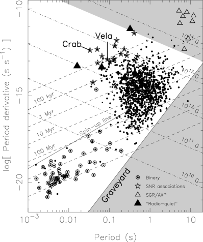
Figure 1: The $P-\dot{P}$ diagram for radio pulsars and magnetars. This is a scatter plot of pulse period and period derivative for pulsars in the current (Apr 2004) public ATNF catalogue. The circled points are pulsars in binary systems while objects in the upper right part of the diagram have derived surface magnetic fields exceeding $B_{\rm q}=4.4\times 10^{13}$ Gauss (see §3.4). The “spin-up” line denotes the terminal period for objects moving to the left in the diagram owing to accretion that become “recycled” pulsars once accretion ceases. The “graveyard” marks the locations where radio pulsars emit less radiation or turn off entirely, possibly associated with the cessation of electron-positron (e^±) pair-production cascades or with saturation of the radio luminosity at some fraction of the total spin-down energy loss rate.

Why perform a full-Galactic census? The Galactic Census is essential in providing the laboratories for a wide range of pulsar applications that will be discussed in more detailed in the following sections. The larger the number of pulsar detections, the more likely it is to find rare objects that provide the greatest opportunities as physics laboratories. These include binary pulsars with black hole companions (see §3.1); binary pulsars with orbital periods of hours or less that can be used for fundamental tests of relativistic gravity (see §3.1); MSPs that can be used as detectors of cosmological gravitational waves (see §3.3); MSPs spinning faster than 1.5 ms, possibly as fast as 0.5 ms, that probe the equation-of-state under extreme conditions (see §3.2); hypervelocity pulsars with translational speeds in excess of $10^{3}$ km s^-1, which probe both core-collapse physics and the gravitational potential of the Milky Way (see §3.10); and objects with unusual spin properties, such as those showing discontinuities (“glitches”) and apparent precessional motions (both isolated pulsars showing ‘free” precession and binary pulsars showing geodetic precession) (see §3.2).

The second reason to perform a full Galactic census is that the large number of pulsars can be used to delineate the advanced stages of stellar evolution that lead to supernovae and compact objects. In particular, with as large a sample as possible, we can determine the branching ratios for the formation of canonical pulsars and magnetars. We can also estimate the effective birth rates for MSPs and for those binary pulsars that are likely to coalesce on time scales short enough to be of interest as sources of periodic, chirped gravitational waves. The latter population can be directly compared to the results of gravitational wave detectors, which will have been operating for a sufficiently long time by the time the SKA is switched on.

The third reason is that a maximal pulsar sample can be used to probe and map the interstellar medium (ISM) in a nearly complete way. Measurable propagation effects include dispersion, scattering, Faraday rotation, and HI absorption that provide, respectively, line-of-sight integrals of the free-electron density $n_{e}$, of the fluctuating electron density, $\delta n_{e}$, of the product $B_{\parallel}n_{e}$, where $B_{\parallel}$ is the LOS component of the interstellar magnetic field, and of the neutral hydrogen density. The resulting measures are DM, SM, RM and $N_{\rm HI}$,

$$\rm DM = \int_{0}^{D}ds\,n_{\rm e},\quad\rm SM=\int_{0}^{D}ds\,C_{\rm n}^{2},$$ (1)

$$\rm RM = \int_{0}^{D}ds\,n_{\rm e}B_{\parallel},\quad N_{\rm HI}=\int_{0}^{D}ds\,n_{\rm HI},$$ (2)

involving quantities that can also be studied by other means, for instance by HI observations with the SKA. The determination of these observables for a large number of independent line-of-sights for pulsars will enable us to construct a complete map of the Galaxy (see §3.7).

With a Milky Way birth rate that currently may be as large as $10^{-2}$ yr^-1, about $10^{8}$ NSs have been formed over the lifetime of the Galaxy, and probably many more because the star-formation was most likely higher in the past. Most NSs are inert, their radio emission having shut off long ago, and up to about half of them will have left the Galaxy owing to their large space velocities. Of the known pulsars (see Fig. 1), we can identify several subclasses:

1. Canonical pulsars: These pulsars, like those first discovered, have present-day spin periods ranging from tens of milliseconds to 8 s and surface magnetic field strengths $B\sim 10^{12\pm 1}$ G. They are often thought to be born with periods $\sim 10$ ms, though evidence suggests that some objects are born with periods longer than 0.1 s [45]. In the standard picture of NS formation, all pulsars start as canonical pulsars. In the $P-\dot{P}$ diagram of Fig. 1 most of these pulsars are located at $P\sim 1$s and $\dot{P}\sim 10^{-15}$. Young pulsars are especially important members of this class because they are associated with supernova remnants and often show copious numbers of glitches.

2. Modestly recycled pulsars: are objects in binaries that survived a first SN explosion and subsequently accreted matter that spun-up the pulsar and reduced the effective dipolar component of the magnetic field. Accretion is terminated in these objects by a second supernova explosion that may or may not disrupt the binary. Those that survive are seen today as relativistic NS-NS binaries. Evolutionarily, it is possible that some surviving binaries include black-hole companions. In the $P-\dot{P}$ diagram of Fig. 1 these pulsars are typically located around $P\sim 30$ ms and $\dot{P}\sim 10^{-18}$.

3. Millisecond pulsars (MSPs): objects in binaries that survive the first SN explosion and in which the companion object eventually evolves into a white dwarf. The long, preceding accretion phase spins the pulsar up to millisecond periods while attenuating the (apparent) dipolar field component to $10^{8}-10^{9}$ G. The consequent small spin-down rates seem to underly the high timing precision of these objects and imply spin-down time scales that exceed a Hubble time in some cases. In the $P-\dot{P}$ diagram of Fig. 1 these pulsars are typically located around $P\sim 5$ ms and $\dot{P}\sim 10^{-20}$. Evolutionary scenarios that produce recycled pulsars and MSPs are discussed in [6].

4. Strong-magnetic-field pulsars: Recently discovered radio pulsars have inferred fields $\mathbin{\lower 3.0pt\hbox{$\hbox to0.0pt{\raise 5.0pt\hbox{$\char 62\relax$}\hss}\mathchar 29208\relax$}}10^{14}$ G [8, 52], rivalling those inferred for “magnetar” objects identified through their X-and-$\gamma$ radiation that seems to derive from non-rotational sources of energy. The relationship between magnetars and these high-field radio emitting pulsars, whose radiation derives solely from spin energy, is not yet known. In the $P-\dot{P}$ diagram of Fig. 1 these radio pulsars are typically located around $P\sim 5$s and $\dot{P}\sim 10^{-13}$.

We envision a full-Galactic census of radio pulsars that aims to detect at least half of the active radio pulsars that are beamed toward Earth (Figure 2). The typical lifetime of canonical pulsars $\sim 10$ Myr, where we define lifetime as the duration of the radio-emitting phase that, for objects with $B\sim 10^{12}$ G, is the time needed for a rapidly rotating object to reach the “death band” on the right-hand side of the $P-\dot{P}$ diagram. At long periods short-ward of the death band, where pulsars spend most of their detectable lifetimes, the beaming fraction $\sim 20$% (e.g. [22]), so the fiducial birth rate implies $\sim 2\times 10^{4}$ detectable pulsars in the Galaxy. Non-canonical classes of pulsars add to these numbers only negligibly because their effective birth rates are smaller by a factor $10^{-4}$–$10^{-3}$.

Figure 2: Simulated Galactic pulsar population discovered in a SKA survey of the enitre sky. The $\sim 20,000$ pulsars shown together with the spiral arms structure. The Galactic Center is located at the origin while the Sun is at (0.0,8.5) kpc.

2.2 Galactic Center

The Galactic Center (GC) is an especially tantalising but exceedingly difficult region to search for pulsars. In many respects, the GC is similar to an especially large globular cluster with regard to the density of stars (cf. §2.3). It differs in that molecular material and, hence, star formation are both much more prominent in the GC than in globulars. Additionally, the $\sim 3\times 10^{6}M_{\odot}$ black hole [64] that underlies the compact radio source, Sgr A*, perturbs space time significantly and is fed episodically by inspiraling gas and stars.

Why find pulsars in the GC? Any pulsars detected in or beyond the GC that are viewed through the region are potentially unique probes of the gas, magnetic field, and space-time of the GC region. First of all, pulsars in the GC can be used to probe the magnetoionic medium along the line-of-sight, including possible detection of the inner scale for electron density turbulence (see §3.8). Second, the initial mass function and overall stellar evolution in the GC is likely to be very different from the rest of the Galaxy. The number and ages of pulsars and their binary membership will provide clues about these areas (see §3.8 and §3.10). Finally, the large stellar density offers the possibility of finding pulsars with stellar black hole companions, allowing unprecedented tests of gravitational theories in the strong field limit and the study of black hole properties. Similar studies will be possible for Sgr A*, the supermassive black hole in the center, if pulsars in compact orbits around the black hole are found (see §3.1). Pulse timing measurements may provide the possibility of measuring the spin of the GC’s central black hole.

At present, none of the known pulsars is within or beyond the GC. The primary reason is that an especially intense scattering region lies between us and the GC at close proximity ($\sim 100$ pc) to the GC [48]. The large scattering has been known since shortly after Sgr A* itself was discovered 30 years ago and it has been probed through angular diameter measurements of OH/IR masers in the GC region and through surveys for background AGNs. The implication for pulsars is that, at a standard search frequency of 1.4 GHz, a pulse emanating from the location of Sgr A* would be broadened to $\sim 300$ s owing to multi-path propagation.

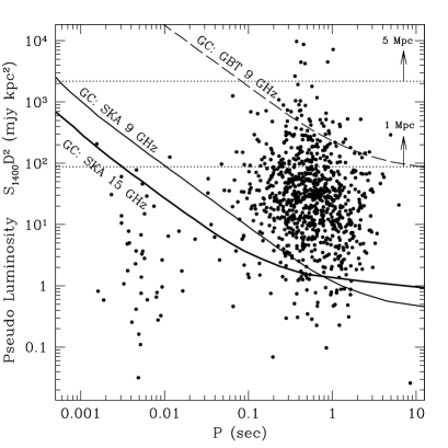
Figure 3: Detectability of pulsars in the Galactic Center and in other galaxies is shown in this plot of “pseudo luminosity” $L_{\rm p}=S_{1400}D^{2}$ vs. spin period for pulsars in the current (Apr 2004) public ATNF catalogue; $S_{1400}$ is the period-averaged flux density at 1.4 GHz. Given duty cycles for pulsars ranging from 0.01 to 0.7, the peak flux density can be a large multiple of the period-averaged flux density. Solid and dashed lines mark the minimum detectable spin period $P_{\rm min}$ for pulsars at the Galactic Center that are detectable with the GBT at 9 GHz and the SKA at 9 and 15 GHz. Scattering is assumed to be in a filled region centered on Sgr A* with $1/e$ cylindrical radius of 0.15 kpc, as included in the NE2001 model. For pulsars at the location of Sgr A*, the dispersion and scattering measures are $\rm DM_{\rm GC}=1577$ pc cm^-3 and $\rm SM_{\rm GC}=10^{7}$ kpc m^-20/3. The curves are based on harmonic sums of the Fourier power spectra of dedispersed time series. They correspond to surveys at these frequencies but have all been scaled to the equivalent sensitivity at 1.4 GHz assuming that the pulsar flux densities scale as $\propto\nu^{-2}$. A bandwidth of 800 MHz was assumed in all cases. Integration times of 1.5 hr and $10^{4}$ s were used for the GBT and the SKA, respectively. In addition, the SKA curves assume that the full sensitivity of the SKA is available. Dotted horizontal lines show the minimum values for $L_{\rm p}$ needed for detection at 1.5 GHz in periodicity searches of pulsars at distances of 1 Mpc and 5 Mpc. The dotted lines assume detectability is independent of spin period, which will not be the case if there is significant scattering along the line of sight.

The pulse broadening time $\tau_{d}$ scales with the observed angular diameter $\theta_{d}$ as $\tau_{d}={W_{\tau}D\theta_{d}^{2}}/{2c}$, where $D$ is the source distance and $W_{\tau}$ is a geometrical weighting factor that takes into account the location of the scattering region relative to the source and observer. For the GC, the weighting factor is very large because the region is much nearer the GC than the observer. For scattering by fluctuations in the electron density, $\theta_{d}\propto\nu^{-2}$ and thus the broadening time is a very strong function of frequency, $\tau_{d}\propto\nu^{-4}$.

To combat pulse broadening, observations at higher frequencies are therefore needed that exploit the strong $\nu^{-4}$ dependence. For example, 10 GHz observations yield $\sim 0.11$s broadening, small enough to allow detection of longer period pulsars. However, pulsar spectra are power-law in form, often with steep dependences $\propto\nu^{-\alpha}$ with $\alpha$ ranging from 0 to 3 and $\langle\alpha\rangle\approx 1.5$. While ongoing searches may yield detections of a few pulsars in the GC, some of which may provide important probes of the region, the sensitivity of the SKA is clearly needed at high frequencies to detect a meaningful sample of pulsars in the GC, as demonstrated in Figure 3. The figure shows the radio luminosity (defined as $L_{\rm p}=$ flux density $\times$ distance²) at 1.4 GHz plotted against spin period along with detection threshold lines for the Green Bank Telescope (GBT) and for the SKA.

The maximum detectable distance is

$$D_{\rm max}=\left(\frac{L_{\rm p}}{S_{\rm min_{1}}}\right)^{1/2}N_{\rm h}^{1/4},$$

where $S_{\rm min_{1}}=mS_{\rm sys}/\sqrt{2BT}$ is the single-harmonic threshold with $m$ = the threshold signal-to-noise ratio, and $N_{\rm h}$ is the number of harmonics detected in the search power spectrum. The minimum luminosity for $m=10$ is thus

$${L_{\rm p}}_{\rm min}=87.5\,{\rm mJy\,kpc^{2}}\left(\frac{D_{\rm max}}{1\,{\rm Mpc}}\right)^{2}\left(\frac{N_{\rm h}}{16}\right)^{-1/2}.$$

For short period pulsars, the number of harmonics detected will be less than the 16 number assumed in this equation.

Also shown in Figure 3 are detection curves for the minimum detectable period $P_{\rm min}$ vs. $L_{\rm p}(1.4\,{\rm GHz})$. These are shown for pulsars at the Galactic Center that are detectable with the Green Bank Telescope (GBT) at 9 GHz and with the SKA at 9 GHz and 15 GHz. These curves were calculated for pulsars near the location of Sgr A* and take into account pulse broadening from scattering and the spectral dependence of the pulsar flux density using a conservative value for spectral index, $\alpha=2$. The detectability was thus calculated for surveys at these frequencies but has been scaled to the equivalent sensitivity at 1.4 GHz. The calculations assume that the full sensitivity of the SKA is available. If only a fraction $f_{c}$ can be used in a blind survey using a “core” array, then the curves will move upward by an amount $\log f_{c}$.

2.3 Globular Clusters

Globular Clusters hold vast reservoirs of MSPs, which are formed at a rate per unit mass which is at least an order of magnitude higher than in the Galactic disk. The reason for this overabundance, which may be even higher than presently seen due to the escape of high velocity objects, is thought to be the formation of binaries via two- and three-body encounters in the high density environments of Globular Clusters.

Why perform a full census of globular clusters? The greatly increased likelihood that many of these MSPs in globular clusters will have undergone some form of dynamical interaction means that the chances of finding exotic binaries, such as the long sought-after MSP-black hole system, are perhaps highest in globular clusters (see §3.1). Furthermore the pulsars in each globular cluster will provide us with exceptional probes of the history and evolution as well as its present properties, including the dynamics, gas content, accurate distances and proper motion (see §3.9). Moreover, an open question is whether globular clusters contain massive black holes in their centers [54, 31], or possibly even binary black holes [12]. Pulsar timing with the precision achievable with the SKA will provide us with a tool to reveal whether such systems are present. This can be achieved either by probing the inner most regions of the cluster to reveal velocities or accelerations expected due to the presence of a black hole, or by using the pulsars in the cluster as an in situ gravitational wave detector sensitive to the presence of binary black holes (see §3.3).

At present there are 76 pulsars known in 23 globular clusters. Not all clusters are equally rich, and it is not clear what determines the number of active pulsars in a given cluster. Based on our knowledge of the luminosity function of the MSPs in the Galactic disk combined with the continuum radio emission and the numbers of MSP-like X-ray sources associated with globular clusters, the total population is likely to be at least two orders of magnitude more than this.

The remaining pulsars in these globular clusters are difficult to find with present instruments due to a combination of the intrinsic low luminosity of MSPs and the typically large distances to globular clusters. Furthermore, most pulsars are in compact binary orbits. Given the presently long integration times needed to detect the pulsars, the pulse signal is often smeared out due to the Doppler effect. Recent developments of sophisticated techniques to correct for this smearing have resulted in an increase in the number of systems known, but blind searches are often too computationally expensive and the vast majority of systems are still too weak for detection.

Targeted SKA surveys of all Galactic globular clusters will enable us to detect all of the pulsars contained therein which are beamed in our direction. This complete census will uncover large numbers of pulsars with which to study their formation, evolution, spin parameters, binary nature and emission properties.

2.4 External Galaxies

Pulsars beyond the disk of the Milky Way are known only in globular clusters and in the Magellanic Clouds owing to their intrinsic faintness. With the SKA, galaxies in the local group, including M31 and M33, are within reach using periodicity searches while giant pulses like those seen from the Crab pulsar can be detected from galaxies out to at least 5 Mpc.

What is the importance of detecting pulsars in other Galaxies? Pulsars likely to be detected will be young pulsars with high luminosities that can be correlated with catalogs of supernova remnants and will yield estimates of the star-formation rate and the branching ratio for supernovae to form spin-driven pulsars as opposed to magnetars and blackholes. Extragalactic pulsars will also provide information about the magnetoionic media along the line of sight through determination of DM, SM, and RM. Unambiguous study of the intergalactic medium in the local group requires removal of contributions to these measures from the foreground gas in the Galaxy and gas in the host galaxy. The more pulsars detected in a galaxy, the more robust this removal will be.

Extragalactic pulsars can be found through blind surveys for both periodic sources and individual giant pulses. Additional successes will follow from targeted surveys of individual supernova remnants in the nearest galaxies. In §4.1 we discuss the requirements on sensitivity and field of view (FOV).

Figure 3 includes detection lines for surveys at 1.4 GHz for pulsars at 1 Mpc and 5 Mpc assuming that the full SKA sensitivity is available. Full sensitivity would apply to targeted searches of, for instance, supernova remnants in nearby galaxies. However, $\sim$full-FOV blind surveys will provide only a fraction $f_{c}$ corresponding to a core array. With full sensitivity, a reasonable fraction of the luminosity function can be sampled out to 1 Mpc and a few pulsars can be detected to 5 Mpc.

Giant pulses from the Crab pulsar serve as a useful prototype for estimating detection of strong pulses from nearby galaxies. The strongest pulse observed at 0.43 GHz in one hour has $S/N_{\rm max}=10^{4}$ – even with the system noise dominated by the Crab Nebula. For objects in other galaxies, the system noise is dominated by non-nebular contributions, implying that the S/N in this case would have increased by a factor of about 300. We can estimate the maximum distance of detection at a specified signal-to-noise ratio, $(S/N)_{\rm det}$ as

$$D_{\rm max} \approx \frac{1.6\,{\rm Mpc}}{\sqrt{(S/N)_{\rm det}/5}}\left(\frac{f_{c}A_{\rm SKA}}{A_{\rm Arecibo}}\right)^{1/2},$$ (3)

where $f_{c}A_{\rm SKA}$ is the SKA’s collecting area that can be used for a giant pulse survey and $A_{\rm Arecibo}$ is Arecibo’s effective area at 0.43 GHz. The usable area for the SKA in a blind survey will be limited by what fraction $f_{c}$ of the antennas are directly connected to a central correlator/beamformer. For $f_{c}=1$, $A_{\rm SKA}/A_{\rm Arecibo}\approx 20$, the standard one-hour pulse seen at Arecibo could be detected out to 7.3 Mpc.

3 Fundamental Physics & Astrophysics

Having discovered a large sample of pulsars in the census of the Milky Way, the Galactic Centre, Globular Cluster and external galaxies, a vast range of fundamental problems in physics and astrophysics can be studied. We highlight some of those in the following.

3.1 Tests of Theories of Gravity

The theory of General Relativity (GR) has to date passed all observational tests with flying colours. Nevertheless, one of the most fundamental questions remaining is whether Einstein’s theory is the last word in our understanding of gravity or not. Solar system tests of GR are made under weak-field conditions, illuminated by the small orbital velocities and gravitational self-energies involved (e.g. the self-energies for the Sun and the Earth, expressed in units of their rest-mass energy, are $\epsilon_{\rm Sun}\sim-10^{-6}$ and $\epsilon_{\rm Earth}\sim-10^{-10}$, whilst for a pulsar and black hole (BH) we find $\epsilon_{\rm PSR}\sim-0.2$ and $\epsilon_{\rm BH}=-0.5$). Therefore, none of these tests of gravitational theories can be considered to be complete without probing the strong-field limit, which is done best and with amazing precision using binary radio pulsars [18]. However, even the existing binary pulsar tests only begin to approach the strong-field regime and the discovery of more extreme binary systems is required. Indeed, the SKA is the only instrument which promises to probe the strong-field limit via the discovery and timing of such systems, in particular that of a pulsar orbiting a BH. The promises provided by the discovery of such particular systems are discussed in detail in a companion key science article (Kramer et al., this volume), where we detail how pulsars can be used to test the “Cosmic Censorship Conjecture” and the “No-hair” theorem for the description of BHs. Here, we concentrate on general aspects of tests of gravitational theories using pulsars timed with the SKA.

Since NSs are very compact massive objects, double neutron star (DNS) binaries can be considered as ideal point sources. Finding and timing DNSs in tight binary orbits – ideally close to coalescence and thus emitting strong gravitational waves – provide stringent tests of theories of gravity in the strong-gravitational-field limit. Tests can be performed when a number of relativistic corrections to the Keplerian description of the orbit, the so-called “post-Keplerian” (PK) parameters, can be measured. For point masses with negligible spin contributions, the PK parameters in each theory should only be functions of the a priori unknown NS masses and the well measurable Keplerian parameters. With the two masses as the only free parameters, the measurement of three or more PK parameters over-constrains the system, and thereby provides a test ground for theories of gravity [17]. In a theory that describes the binary system correctly, the PK parameters produce theory-dependent lines in a mass-mass diagram, which compares the masses of the two neutron stars, that all intersect in a single point.

The best example for such tests is currently given by the double pulsar system PSR J0737$-$3039 where five PK parameters are available for tests, in addition to the theory independent mass ratio of the two NSs [51]. For the relativistic binary systems that will be discovered and timed with the SKA, one would be able to routinely measure five or more PK parameters, severely over-constraining the system. In particular, more double pulsar systems will be found, and PK parameters that are currently impossible (or extremely difficult) to measure, such as those arising from aberration effects and geodetic precession, would become accessible with the SKA, providing also full 3-D information about the orientation of these binary systems.

Most importantly, current PK parameters are only measured to the lowest post-Newtonian approximation. The timing precision achievable with the SKA means that higher-order corrections are likely to become important, demanding the development of a timing formula that is accurate to at least second post-Newtonian order. For instance, corrections would need to account for the assumptions currently made in the computation of the Shapiro delay (see §3.2) that gravitational potentials are static and weak everywhere [83, 43, 44]. In addition, other effects such as those related to light bending and its consequences will become important where an additional signal would be superposed on the Shapiro delay as a typically much weaker signal, which arises due to a modulation of the pulsars’ rotational phase by the effect of gravitational deflection of the light in the field of the pulsar’s companion [20].

Like the DNS binaries, most NS-white dwarf (NS-WD) binaries can also be considered as pairs of point masses. Significant measurements of PK parameters can only be obtained in a few cases so far, since relativistic effects for NS-WDs are generally much smaller than for DNS binaries (e.g. [80, 2]). However, with the SKA, PK parameters can be determined for many more systems. Such measurements can be similarly valuable since NS-WD systems test different aspects of gravitational theories. For instance, as shown recently [23], the tests provided by the PSR-WD system J1141$-$6545 are more constraining for the class of tensor-scalar theories than those tests provided by the double pulsar. The reason is that unlike GR, some alternative theories of gravity, such as tensor-scalar theories, predict effects that depend strongly on the difference between the gravitational self-energy of two orbiting bodies, which is large in NS-WD systems. Using such systems, one is able to probe possible violation of conservation of momentum, equivalence principles and expected Lorentz- and positional invariances [73]. A manifestation of such effects would, for instance, be measurable in the detection of gravitational dipole radiation where as GR only predicts quadrupole emission.

The computer power available when the SKA comes online will enable us to do much more sophisticated searches in parameter space, including full searches in acceleration due to binary motion, than possible today, and the SKA sensitivity allows much shorter integration times, so that searches for compact binary pulsars will no longer be limited. Hence, the combination of SKA sensitivity and computing power means that the discovery rate for relativistic binaries is certain to increase beyond the number of at least a hundred compact binary systems that we can expect from an extrapolation of the present numbers.

In summary, tests of gravity affordable with the SKA will not simply be a continuation of the present tests at higher precision levels, but the better sensitivity and timing precision will enable us to perform genuinely new tests. These prospects arise from the assumption that the timing precision can be improved by two or even three orders of magnitude over the current standards. However, as we discuss in some detail in §4.3, this requires not only an increase in raw sensitivity but also the ability to correct for propagation effects from intervening plasmas and sufficient polarization purity and (quasi-) simultaneous multi-frequency observations. Moreover, the intrinsic phase-jitter of pulsars will prevent the timing precision of some MSPs from reaching the theoretical limit given by radiometer noise, so that the application of correction schemes needs to be considered on a case-by-case basis. However, the current timing precision of a number of MSPs appears to be limited by telescope sensitivity, as opposed to systematic effects (e.g. [81]), suggesting that much improved timing precision can be achieved for a few objects and that new, unique tests of relativistic gravity will be enabled through greater telescope sensitivity.

It is important to note that many of these experiments require corrections of the measured parameter values for kinematic effects. For instance, the precision of GR tests achievable with PSR B1913+16 is limited by the accuracy to which the pulsar’s motion and acceleration in the gravitational potential of the Galaxy is known [82]. Observed values for parameters like the orbital decay rate, $\dot{P}_{\rm b}/P_{\rm b}$, or changes in the semi-major axis, $\dot{x}/x$, are affected by a kinematic Doppler term given by [17]

$$-\frac{\dot{D}}{D}=\frac{1}{c}\>\vec{K}_{\rm 0}\cdot(\vec{a}_{\rm PSR}-\vec{a}_{\rm SSB})+\frac{V_{T}^{2}}{c\>d}\;,$$ (4)

where $\vec{K}_{\rm 0}$ is a vector from the Solar System Barycentre (SSB) towards the binary pulsar, $\vec{a}_{\rm PSR}$ and $\vec{a}_{\rm SSB}$ are the Galactic accelerations at the location of the binary system and the SSB. The last term including the transverse velocity, $V_{T}$, and distance, $d$, to the pulsar is known as secular acceleration or “Shklovskii term” [70]. Correcting for this term to derive the intrinsic values obviously requires precise astrometric information like proper motion and distances which can be derived using the VLBI capabilities of the SKA. In order to get precise distances for pulsars across the Galaxy a final positional accuracy of 0.1 mas is needed at 5 GHz.

3.2 Structure of Neutron Stars & Equation-of-State

The internal structure of NSs is complex. This question was already addressed by Oppenheimer & Volkov (1939) long before the discovery of pulsars. The structure depends sensitively on the equation of state, i.e. the relationship between density and pressure. Knowledge of the exact equation of state would allow us to deduce most of the NS’s physical properties, most notably its radius for a given mass. With the SKA we can address this question from various angles.

Firstly, the study of the equation of state will benefit from the vastly improved statistics of observed pulse periods. Periods of known pulsars range from 1.5 ms to 8.5 s. The discovery of even smaller rotational periods will provide significant insight into the properties and stiffness of the ultra-dense liquid interior of NSs. Even the case of a “null result”, that no period shorter than 1.5 ms will be found, will require a theoretical explanation, as it requires the existence of a limiting period not far away from the currently observed value but larger than our current theoretical limits. At the other extreme end, the discovery of very long period pulsars, isolated or in binary systems, will establish the connection of radio pulsars to magnetars, Soft-Gamma ray Repeaters (SGRs) and Anomalous X-ray Pulsars (AXPs), clarifying as to whether these are distinct classes of NSs or simply different evolutionary stages or end products (see also §3.4).

Secondly, observations of relativistic effects in binary pulsars allows precise determinations of the masses of the pulsar and its companion. This is possible when either two or more PK parameters can be determined (see §3.1), or when a Shapiro delay can be measured. The Shapiro delay in the arrival time of a pulse arises from the curvature of space-time caused by the presence of a companion star. Measuring the Shapiro time delay is therefore the most straightforward way to obtain a direct measurement of the companion mass and, hence, of the mass of the active pulsar from knowledge of the total system mass (e.g. by measuring a relativistic precession of the orbit). Currently, the masses of about 20 neutron stars can be determined (Fig. 4). With hundreds of NS mass measurements available, the range of observed masses can be studied and related to the spin periods, promising to reliably establish the maximum possible mass of observable NSs. Moreover, the observed values can be related to the evolutionary history of the binary systems, studying the amount of matter accreted during a spin-up process as an X-ray binary. Given that some millisecond pulsars are very old, one may also be able to put limits on the evolution of NS masses with age of the universe, so that variations in the gravitational constant can be detected or constrained [77]. It is also worth pointing out that, in addition to precisely measuring the distribution of masses of NSs, the same observational techniques can be used to obtain mass measurements of other compact pulsar companions. The current timing precision usually prevents this, but with the SKA it would be possible to perform such measurements also for WD companions. [74]

Figure 4: Mass measurements of neutron stars obtained from the timing of binary pulsars with corresponding uncertainties shown. The canonical value of 1.4$M_{\odot}$ is indicated by the vertical line. While mildly recycled and young pulsars are broadly consistent with this value, millisecond pulsars born in the process of a prolonged mass transfer appear to have somewhat larger masses. Figure compiled by Stairs (2004).

Thirdly, the moment of inertia of NSs can be determined when high precision timing observations allow the detection of relativistic spin-orbit coupling in DNSs. This effect would be visible most clearly as a contribution to the observed periastron advance in a secular [4] and periodic fashion [85]. The size of the contribution depends on the pulsars’ moments of inertia, which therefore can be determined if two other PK parameters can be determined with sufficient accuracy so that the effect of spin-orbit coupling can be isolated [16]. The SKA timing precision will be crucial in pushing the measurement accuracy to the limits required to see this effect of second Post-Newtonian (i.e. $(v/c)^{4}$) order (cf. §3.1).

Finally, observations of rotational instabilities in pulsars, which include rapid spin-ups followed by slow relaxation — glitches — and stochastic variations generically called timing noise, probe the interior of NSs in a unique way that can be considered “neutron star seismology”. Observations of glitches and their recovery provide strong evidence for the existence of a fluid component inside the solid outer crust of the NS, providing the basic picture of NS structure provided in the introduction. This picture is based on only a small number of glitches observed in even fewer pulsars (e.g. [69]). The reason is that glitches – mostly observed in young pulsars – are rare, so that their timely detection is important to follow the revealing relaxation process. With the SKA a large number of pulsars would be monitored simultaneously, so that glitches can be observed as they happen. The multi-beam capabilities of the SKA are essential for this study.

The results obtained from the analysis of the detected glitches can be compared to the observations of pulsars that are found to be freely precessing, since the time-scales for precession are probably related to the coupling-strength between the liquid interior and the solid crust. Currently, convincing evidence for free precession is found for only a few pulsars [72], but SKA timing observations of all pulsars discovered in the cosmic census will produce further examples.

Timing noise constitutes stochastic variations in pulse phase residuals (e.g. after removing spin-down polynomial components and orbital effects) that show non-stationary statistics and is thus often described as having a “red” power spectrum. It is radio-frequency independent (after any DM and scattering variations from the ISM are subtracted) and appears to be caused by torque variations acting on the NS crust. It is possible that some or all timing noise is associated with free precession induced by crust quakes that cause misalignment of the angular momentum vector and the spin axis. This conjecture can be tested only by identifying more objects that show pulse shape variations caused by wobble of the radio beam that accompanies pulse phase variations.

3.3 Pulsars as sources and detectors of gravitational waves

Pulsars are not only detectable across the whole electromagnetic spectrum, but rotating and coalescing NSs are also among the sources expected to be detected first with gravitational wave (GW) detectors.

The recent discovery of the J0737$-$3039 system suggests that Advanced LIGO, operating on timescales similar to those for the SKA, will detect a few coalescing binary pulsars each day [7, 39]. Moreover, it is anticipated that J0737$-$3039 can act as a calibrating signal for the space interferometer LISA. The SKA will discover many more such compact relativistic binaries and will hence provide key information for a location and study of these objects in a non-photonic window.

Moreover, deviations from a purely spherical shape will cause spinning NSs to emit continuous GW emission that may even be detected with current generations of GW telescopes like LIGO, GEO600 or VIRGO. The faintness of the signal requires knowledge of the precise positions and spin-frequencies of the pulsars. With the majority of Galactic pulsars potentially being discovered with the SKA (see §2.1), sensitive targeted GW searches are possible for a very large number of pulsars, so that the actual shape of a NS can be probed.

As a result of the cosmic census, the SKA will also produce a dense array of millisecond pulsars across the sky. Being timed to very high precision ($\mathbin{\lower 3.0pt\hbox{$\hbox to0.0pt{\raise 5.0pt\hbox{$\char 60\relax$}\hss}\mathchar 29208\relax$}}100$ ns), these act as multiple arms of a cosmic GW detector when a passing gravitational wave perturbs the metric and hence affects the pulse travel time and the measured arrival time at Earth [19, 25, 60]. This “device” with the SKA at its heart – the so-called “Pulsar Timing Array” (PTA) – will be sensitive to GWs to frequencies of 1/observing time, hence $\sim$nHz. The PTA thereby complements the much higher frequencies accessible to Advanced LIGO ($\sim$100Hz) and LISA ($\sim$mHz), and the extremely low frequencies probed by polarization studies of the Cosmic Microwave Background ($\sim 10^{-18}$ Hz).

The measurement precision and accuracy of the pulsar clock is not sufficient to detect the gravitational radiation of stellar-mass binaries by the means of a PTA. However, super-massive black hole binaries in nearby galaxies with orbital periods of a few years would produce a periodicity in pulsar arrival times with an amplitude of the order of 10 ns to 1 $\mu$s and in a frequency range that is detectable with SKA timing [60, 49]. The light-travel time delay between the Earth and the timed pulsars can, depending on the geometry, enable us to observe a given massive binary system at two different epochs simultaneously. A slow decay of the binary orbit hence results in both low and high frequency components of the timing residuals, whereas the difference in the frequencies of these components will depend on the orbital decay rate. As pulsar timing is more sensitive to lower frequencies, the highest amplitude oscillations in the timing residuals will be due to the delayed component. This effect corresponds to the three-pulse response occurring in spacecraft Doppler tracking experiments and the multi-pulse response from time-delay interferometry used with LISA [36].

The short lifetime of such massive binaries reduces the chances of detecting such systems. In contrast, the SKA can detect the signal of a stochastic background of gravitational wave emission produced by a large number of unresolved independent and uncorrelated events. Another contribution to the GW background, but with a different spectrum, is expected in some cosmological string theories. The SKA is crucial in answering the question about the existence, nature and composition of a stochastic GW background. The construction of a PTA to detect such signals is one of the key-science projects of the SKA and is presented in more detail in the contribution by Kramer, this volume.

3.4 Relativistic Plasma Physics

The plasma physics occurring under extreme conditions of very high densities, super-strong magnetic fields and in the rather complex environment known as the pulsar magnetosphere are only poorly understood. This situation remains after almost 40 years of pulsar research and is in spite of the large number of studies and observations devoted to the identification of the relevant physical processes (e.g. [53]). Solving this “pulsar problem” however offers deep insight into relativistic plasma physics, and the SKA may provide us finally with the observational facts to understand pair production processes, the creation of radio and high-energy emission and the overall structure of the pulsar magnetosphere.

Radio Fluctuations: The size of the region of electromagnetic activity around active pulsars, the magnetosphere, is essentially the light-cylinder radius,

$$R_{\rm LC}=\frac{c}{\Omega}=\frac{cP}{2\pi}\simeq 4.77\times 10^{4}\;\mbox{km}\;\left(\frac{P}{\rm s}\right).$$ (5)

Radio emission altitudes are much smaller than $R_{\rm LC}$ and radio emission is expected to originate as close to the NS surface as 10-100 stellar radii, produced by a relativistic pair plasma that is created in the polar gap region [46].

While pulsars are renowned for their stable average pulse profiles formed by the summing together of many pulses, single pulses provide us with the rich detail that reflects the physics of the generation and propagation of radio emission. The initially chaotic appearance of single pulses can often be resolved to reveal a rich phenomenology that includes: drifting sub-pulses, nulling, microstructure and giant pulses which correspond to the building blocks of the observed pulsar radiation (e.g. [79, 32]). Key tests of all emission mechanisms and the role of the magnetosphere therefore come from determining the instantaneous time duration and evolution, the frequency bandwidth and the polarisation properties of these phenomena. However, our understanding of how this phenomenology reflects the underlying physics has been restricted because radio emission from pulsars is weak and presently there are only a limited number of sources in which single pulses can be studied (e.g. [40]). The unprecedented leap forward in sensitivity combined with sky coverage provided by the SKA will revolutionise the study of single pulses. To complete this study, instantaneous coverage of a very wide band (e.g. 0.1 to 5 GHz or higher) is desireable so that individual pulses can be tracked. This specification surpasses the strawman 20% bandwidth specification for the SKA but would allow new approaches to the understanding of pulsar magnetospheres.

Relationship to Magnetars and Other Objects: The SKA will also provide the sensitivity to test whether “radio-quiet” objects like magnetars are in fact very weak radio emitters. The pair cascade processes that seem to be relevant to create the radio emitting plasma may be prevented if the magnetic field strength at the polar cap exceeds the critical magnetic field

$$B_{q}=m_{e}^{2}c^{3}/e\hbar=4.4\times 10^{13}\;\mbox{\rm G}.$$ (6)

For magnetic fields of such strengths, other processes may compete with magnetic photon splitting, changing the opacity of the gap region. Such arguments have been used to explain the absence of radio emission from magnetars [3], but these models have been challenged by the discovery of high magnetic field radio pulsars [8, 52]. The SKA can both establish whether magnetars are weak radio emitters as well as discover more radio-loud pulsars with spin-parameters similar to those of magnetars, so that the question about the relationship between pulsars and these prominent high-energy sources can be settled. As the Galactic menagerie of pulsars grows, additional classes of objects may also be identified, such as young NSs with anemic magnetic fields that appear to be lacking on the left side of the $P-\dot{P}$ diagram.

The Radio-High-Energy Connection: Regularly pulsed high-energy emission is known for an increasing sample of radio pulsars [76]. As for the radio emission, the origin of the high-energy emission is still a matter of significant debate. Likely emission processes for the observed non-thermal optical, X-ray and $\gamma$-ray emission are synchrotron emission, curvature emission and inverse Compton scattering. The location of this emission is thought to be either in the polar cap region (e.g. [33]) or in the outer gaps (e.g. [10]). In both families of models, the high-energy emission beam appears to be much wider than the radio beam. With upcoming missions like GLAST, the high-energy emission of pulsars will be much better understood by the time observations with the SKA can be made. Then, however, the SKA can be used to probe the relationship between high-energy and radio emission, so that a coherent model of the active magnetosphere can be developed. Current results suggest that the high energy emission may indeed be related to some of the radio emission properties (e.g. [62]).

A radio-high-energy link is provided by the phenomenon of giant radio pulses. All pulsars with detected giant-pulse emission are also detected at high energies [37]. Another common feature these pulsars share is the high magnetic field strength at their light cylinders [11]. Interpretation of this correlation is unclear at present. Giant pulses often occur misplaced from the normal radio profile but appear to be aligned with X-ray and/or $\gamma$-ray emission (e.g. [62]). This suggests a common origin of the giant pulses and high-energy emission and indicates that some observed radio emission could be in fact a by-product of the high-energy radiation process. This could explain highly unusual high radio-frequency components, seen to emerge at atypical pulse phases in the Crab profile at a few GHz [55]. Observations also suggest that optical pulses of the Crab pulsars occurring simultaneously with radio giant pulses appear to be somewhat brighter than other optical pulses [67].

With its sensitivity and monitoring capabilities, the SKA can detect giant pulses simultaneously at many radio frequencies, allowing us to determine the spectrum and their relationship to the high energy emission. This observational mode is identical to the requirements for the study of the “Dynamic Radio Sky” (see second contribution by Cordes, this volume), as giant pulse emission is the prototype for transient coherent emission. Due to their strength, giant pulses can be detected from sources as far away as the Virgo cluster and can be used to directly target young NS in the Milky Way and nearby galaxies, as discussed in §2.4.

3.5 Resolving Pulsar Magnetospheres

The SKA can provide the means to actually resolve the pulsar magnetosphere. At a typical distance (1 kpc), the light cylinder radius has an angular scale $\theta_{\rm LC}\approx 0.32PD_{\rm kpc}^{-1}\,{\rm\mu arcsec}$. Actual radio emission altitudes are much smaller than $r_{\rm LC}$ and light-travel-time arguments suggest emission sizes of 2-ns duration nano-Giant pulses [32] about the size of a beach ball, though relativistic motion toward the observer enlarges this by a factor $\gamma\sim 10^{3}$. Conventional interferometry has no hope of resolving the relevant scales. However, interstellar scintillations (ISS) can probe pulsar emission regions. Just as stars twinkle while planets do not because the critical angular size for atmospheric optical scintillation is about 1 arcsec, the critical angular size for ISS $\approx 10^{-7}$ arc sec. Through appropriate measurements of the diffraction pattern caused by interstellar scattering, the phenomenon may be used to constrain emission region sizes and locations. In particular, the dynamic spectrum $I(\nu,t)$ shows structure in time and frequency that may differ between different pulse components. While this method has been applied to a few pulsars, the number of objects is severely limited by sensitivity: the pulsar’s flux must be detectable in a narrow frequency channel ($\sim 1$ kHz) in a short time ($\sim 10$ sec). Also, because the scintillation characteristic bandwidth and time scale are strongly frequency dependent, flexibility in choosing the observation frequency and spectrometer resolutions is needed along with large sensitivity. As with single-pulse studies, very wide instantaneous frequency coverage is important for following the frequency evolution of ISS and intrinsic effects. With the SKA, similar observations will be possible for a large number of pulsars, therefore contributing to the final solution of the pulsar problem. Further discussion on resolving magnetospheres may be found in “The Microarcsecond Sky and Cosmic Turbulence,” (Lazio et al., this volume).

3.6 Extrasolar Planets

The first extrasolar planetary system found is around the pulsar PSR B1257$+$12 [86]. The system consists of (at least) three planets, planet A with approximately a lunar mass, planet B with a mass of $4.3\pm 0.2M_{\oplus}$, and planet C with a mass of 3.9 $\pm 0.2M_{\oplus}$ [42]. Since then, a planet has also been found around the pulsar PSR B1620$-$26 [68, 61], in the globular cluster M4.

While planetary systems around main-sequence stars had been long anticipated and numerous such systems have been found since, pulsar planetary systems were not expected. Although it is unlikely that the number of pulsar planetary systems will ever approach the number of planetary systems around main-sequence stars, pulsar planetary systems offer unique insights. Taken together the two pulsar planetary systems already indicate that planets can form in a wide variety of environments. Already, for instance, the planet around PSR B1620$-$26 challenges conventional notions about the formation of planets. It is thought to have been acquired by the pulsar during a dynamical exchange within the globular cluster, implying that this planet has existed for a substantial fraction of the age of the globular cluster M4. This is a low-metallicity globular cluster, suggesting that planets can form in low-metallicity environments. In contrast, planets orbiting main-sequence stars near the Sun are found almost exclusively around stars with solar- or super-solar metallicities [29, 63], which has led to the belief that only stars with large metal contents can host planets. Similarly, the presence of terrestrial mass planets around PSR B1257$+$12 suggests that terrestrial planets will be widespread, a prediction to be tested by future space missions such as Kepler [41] and the Terrestrial Planet Finder [5].

In addition to probing the details of planetary formation, identification of additional planetary systems around pulsars could provide valuable clues about pulsar formation and evolution and probe similarities and differences between planetary systems around pulsars and main-sequence stars.

The existence of planets around a pulsar is ascertained from the times of arrival (TOA) of pulses over a multi-year time span. The pulsar’s reflex motion in its orbit about the system’s barycentre causes the pulse TOAs to be delayed or advanced relative to what one would predict for an isolated pulsar. Thus, finding additional pulsar planetary systems will require long, high-precision timing observations. Figure 5, however, demonstrates that asteroid-sized objects and smaller can be found with SKA timing.

Figure 5: Planetary companions that can be detected with pulsar timing observations for different values of timing precision. With the SKA a routine timing precision of $\mathbin{\lower 3.0pt\hbox{$\hbox to0.0pt{\raise 5.0pt\hbox{$\char 60\relax$}\hss}\mathchar 29208\relax$}}1\mu$s is anticipated for millisecond pulsars. Currently detected planets using optical methods are shown for comparison.

3.7 Mapping the Milky Way

The goal of a Galactic pulsar census is to detect a large fraction of the roughly $2\times 10^{4}$ pulsars that are beamed toward Earth, or about an order of magnitude larger number of pulsars from current and near-term pulsar surveys. This census will necessarily determine the DMs for all of the pulsars as part of the discovery process, along with estimates for the scattering and rotation measures (SM, RM) of a sizable fraction of the objects in follow-up observations. We expect that the SKA will enable a large increase in the number of pulsar parallaxes, as discussed below.

The number of sampled lines of sight will be sufficiently large and dense on the sky so as to permit qualitatively new models of the Galaxy to be developed. The current “state of the art” model for the Galactic distribution of the warm ionized medium is the NE2001 model [14, 15]. This model describes the Galaxy largely in terms of a small number of smooth, large-scale components. However, it also incorporates a number of electron density enhancements (“clumps”) and voids along the line of sight to a limited number of objects (primarily pulsars). These clumps and voids are required because the various observables for these objects (typically pulsar DMs) cannot be reproduced by only large-scale components.

We envision that, with the Galactic pulsar census provided by the SKA, it will be possible to trace the Galaxy’s structure, or at least its spiral structure, in a self-consistent manner, rather than by imposing it as has been done for the NE2001 and previous models. Parallaxes will be determined for large numbers of pulsars, providing crucial DM-independent distance measurements by which to calibrate the local interstellar medium. Parallaxes will be measureable for some pulsars out to $\sim 10$ kpc distances. For many pulsars, HI absorption can be measured, yielding distance constraints and information on fine structure in the neutral ISM. At larger distances, there should be several pulsars per degree along the Galactic plane. Their lines of sight will have a reasonable probability of intersecting an H ii region even over Galactic distances ($\sim 10$ kpc). The methodology for constructing the model would be to insert clumps of increased electron density, representing H ii regions, along the line of sight to pulsars. The clumps would be inserted in a parsimonious manner so as to minimize the difference between observed and predicted DMs. Combined with the parallax measurements and constraints obtained from scattering measurements of pulsars and extragalatic sources, it may be possible to identify patterns in the locations of clumps that would then reveal the spiral arms. Additional discussion of such modelling is in “The Microarcsecond Sky and Cosmic Turbulence,” (Lazio et al., this volume).

3.8 Mapping the Galactic Center

As is the case for the Galaxy as a whole, detecting pulsars in the GC will allow the magnetoionic medium there to be mapped. However, several novel aspects of the GC result in the potential for additional information to be obtained. Firstly, the geometrical weighting factor for scattering, $W_{\tau}$, can change by large amounts for pulsars at different distances along the line of sight. For instance, two pulsars in the GC separated by only 50 pc along the line of sight ($<1$% of the total distance to the GC) may have pulse broadening times that differ by 25%.

Secondly, gas motions in the GC can be large, in excess of 100 km s^-1 [65]. In contrast to typical observations through the Galactic disk, for which pulsar velocities dominate, in the Galactic center, pulsar and gas velocities may be similar. If the pulsar and gas velocity vectors are anti-aligned, changes in pulsar DMs or scattering parameters could happen on much shorter time scales than are obtained in the Galactic disk. In 1 yr the line of sight through a gas cloud could sweep out of order 100 AU, allowing the AU-scale structure of gas clouds in the GC to be probed.

The distribution of pulse periods that can be detected toward the GC clearly will be affected by scattering (c.f. Figure 3). Nonetheless, a careful accounting for selection effects may allow the pulse period distribution to be used to estimate the past star formation rate in the GC [50]. Even modest constraints on the past star formation rate would be valuable for assessing the extent to which the Galaxy’s nucleus has undergone episodes of star bursts and their magnitude.

Finally, one aspect of the SKA’s Key Science Project on strong-field tests of gravity is to map out the space-time around a black hole. At a crude level, the distribution of period derivatives of pulsars around the black hole could be used to map out the gravitational potential on the large scales around the center. More exciting is the possibility that pulsars will be found sufficiently close to Sgr A^∗ that strong-field gravitational effects, like strong micro-lensing or large time delays, will be measurable [59, 84, 58]. In order to exploit this possibility for GC pulsars, the line of sight to the pulsar must pass within a few Einstein radii of Sgr A^∗, or within roughly $0.\!\!^{\prime\prime}1$. Consequently, only pulsars within the central stellar cluster, or those behind the GC with a favourable projection, will be useful for such strong-field tests.

3.9 Mapping Globular Clusters

The dynamical and stellar evolutionary histories of globular clusters are inexorably linked through the initial binary fraction. The discovery of tens to hundreds of pulsars in these clusters by the SKA, combined with the precise timing it will afford, provides an excellent tool to study these histories. As globular clusters are also thought to play a vital role in galaxy evolution, an improved understanding of their formation and history is of importance. Recent work on 47 Tucanae (e.g. [28]) and NGC 6752 (e.g. [24]) has highlighted this potential, in particular when the knowledge obtained at radio frequencies is combined with results from X-ray observations (e.g. [30]).

Using the measured period derivatives of millisecond pulsars it is possible to measure the line-of-sight acceleration imparted to the pulsars, as this is usually dominated by the gravitational field of the globular cluster. When combined with accurate positions and, possible with the accuracy of SKA timing, accurate parallaxes, this will lead to the best possible determination of the gravitational field. Via the mass density distribution and optical observations, the population of non-optically active cluster members, in particular massive black holes, can be derived. The resultant model of the gravitational potential of the clusters can then be used to determine the ”true” period derivatives of the pulsars and thus their spin-down energies, magnetic field strengths and ages and also correct any measured orbital period derivatives.

The more accurate measurement of the gravitational potentials in these systems will also allow improved modelling of the influence of binaries on the collapse or otherwise, as well as determinations of how many pulsars have potentially escaped the cluster and thus the initial binary fractions. It will also determine what fraction of NSs have escaped these systems and in turn how many of the NSs in the Galaxy originated in globular clusters.

The stars in the globular clusters in our Galaxy span a large range of metallicities and a complete census of pulsars in a large number of globular clusters will therefore provide vital input in determining the stellar evolutionary history of clusters and in particular how the massive end of the initial-mass function depends on metallicity. Differences in the measured dispersion measures of pulsars in globular clusters combined either with models of the potential, or parallaxes, can be used to probe the gas content of the clusters ([27]). The gas, originating from the winds of evolved stars, is expected to be stripped from the cluster, each time the cluster passes through the Galactic plane every $\sim 10^{8}$ years ([71]). The amount of gas determined for various clusters may therefore provide information about the dynamics of the cluster as a whole.

The study of cluster dynamics is supported by the determination of the proper motions of the large samples of pulsars. This will allow accurate determinations of the proper motion of the globular clusters themselves and thus, when combined with optical proper motions, will provide excellent ties between radio and optical reference frames.

3.10 Pulsar Demographics and Core-Collapse Physics

The currently known $\sim 1700$ pulsars represent just the ‘tip of the iceberg’ of a much larger population of perhaps $10^{5}-10^{6}$ active pulsars in the Galaxy. The current sample, biased by selection effects and sensitivity limitations, does not allow answers to a number of important questions that include:

• How many pulsars are in the Galaxy, what is the birth rate, and is there evidence for an increased birth rate in the past?

• Are neutron stars formed preferentially in spiral arms?

• How many pulsars are in globular clusters?

• Do the magnetic fields of isolated neutron stars decay?

• What are the minimum and maximum spin periods for radio pulsars?

• What is the relationship between core collapse and neutron star birth properties?

• How are isolated millisecond pulsars produced?

The properties of the population of pulsars discovered in the Galactic census (§2.1), combined with the statistics of the discovered globular cluster (§2.3) and extragalactic pulsars (§2.4), will unlock the answers to these questions.

The outcome of the Galactic Census and future high-energy studies will establish the relationship between the different manifestations of NSs, i.e. active radio pulsars, “radio-quiet” spin-powered X-ray pulsars, and Soft-Gamma-Ray Repeaters and Anomalous X-ray Pulsars known as magnetars (see also §3.4).

Most (if not all) NSs derive from Type II, core-collapse supernovae. Evidence supports the idea that the collapse and ensuring explosions are not symmetric, thus imparting a translational momentum impulse or “kick” and, perhaps, an angular momentum kick that determines the initial spin state of the NS. The large translational motions of pulsars, $\langle V\rangle\sim 500$ km s^-1 represents firm testimony to this picture, with corroboration from X-ray jets that are aligned with the spin axes in the Crab and Vela pulsars and also with the proper motion vectors. While collapse kicks seem to underly large pulsar velocities, the detailed mechanism for producing kicks is not yet identified [47]. Candidate rocket effects include neutrino emission and mass ejection during NS formation, which may be altered by the magnetic field strength that most likely grows during the collapse. A slower-acting electromagnetic rocket (the Harrison-Tademaru effect) may occur if NS are born spinning fast ($P_{\rm initial}\sim 1$ ms) and if the magnetic field is off axis. In addition it is not known if the velocity distribution has been sampled well enough in the high-velocity component to determine the maximal space velocity and thus the degree of asymmetry.

With the SKA, comprehensive surveys for pulsars with followup astrometry (from interferometry) and polarization measurements will allow a much better understanding of the empirical properties of the pulsar population with regard to kicks and presumably to identification of the processes that underly them. Information will come from determining parallaxes and full 3-D velocities by using the timing and VLBI capabilities of the SKA. Whilst it is currently impossible to determine radial velocities for pulsars (unless in orbit with an optically detectable companion), this will become possible with the SKA for at least a number of pulsars since the affordable timing precision will allow us to detect motion on the sky that is non-linear in time because it results from the three-dimensional spatial motion of the pulsar projected onto the celestial sphere.

4 Technical Requirements

The key observations to achieve the outlined science goals can be summarized as

• Full Galactic and extragalactic censuses of the pulsar population by sensitive searches of the whole sky, the Galactic plane, and specific targets such as the Galactic Center, Globular Clusters or external galaxies.

• Regular multi-frequency timing observations of the $\mathbin{\lower 3.0pt\hbox{$\hbox to0.0pt{\raise 5.0pt\hbox{$\char 62\relax$}\hss}\mathchar 29208\relax$}}10^{4}$ discovered pulsars closely spaced in time in about bi-weekly intervals.

• Targeted observations and dedicated studies of individual objects and/or areas of special interest.

• VLBI observations of a large number of sources to determine their astrometric parameters.

We discuss the technical requirements for these observing programmes in more detail in the following.

4.1 Search Observations

Yields of pulsar searches need to consider propagation effects and binary motion in addition to distributions of spin periods, luminosities and distances of target populations. For both single-pulse and periodicity searches, algorithms approximate matched filtering procedures on the signal.

The main requirements for pulsar searches are

1. A configuration that allows a significant fraction of the total SKA’s collecting area to be used in blind surveys that sample a wide field (e.g. at least 1 deg² at 1 GHz).

2. Frequency coverage that allows optimal detection of pulsars in periodicity and single-pulse searches for most Galactic and extralagalactic lines of sight (e.g. 0.5 to 5 GHz) and also for the highly scattered Galactic Center region, which requires 9 to 15 GHz.

3. Wide bandwidth with adequate channelization to allow dedispersion. Dispersive smearing across a channel is

   $$\Delta t_{\rm DM}=\frac{8.3\,\mu s\rm DM\Delta\nu_{\rm ch}}{\nu^{3}},$$ (7)

   for $\Delta\nu_{\rm ch}$ and $\nu$ in MHz and GHz, respectively. DM ranges up to 1200 pc cm^-3 in the known sample and values as large as several thousands are expected for some lines of sight. Assuming 20% fractional bandwidth (an underestimate at 1-2 GHz frequencies), the number of channels needed in post-detection dedispersion is

   $$N_{\rm ch}\approx\frac{1600}{\nu^{2}}\left(\frac{\rm DM_{\rm max}}{10^{3}\,{\rm pc\,cm^{-3}}}\right).$$ (8)

   At low frequencies or high DM, dedispersion is best done coherently, requiring access to the pre-detection baseband signal. For coherent dedispersion, the only extrinsic smearing effects are from interstellar scattering and instrumentation. The signal processing burden is quite large for coherent dedispersion, however, and will require state-of-the-art processors to achieve desired bandwidths.

4. Time resolution sufficient to sample the shortest pulse widths.

5. Flexibility of the correlator/beam-former to provide the above sampling.

We quantify the collecting area usable in pulsar surveys as the fraction $f_{c}$ in a “core” array with which full-FOV sampling can be performed. In some designs, the core array would correspond to those antennas whose signals can be directly correlated (as opposed to being combined in a beamformer first). The system-equivalent flux density for the core array is $S_{\rm sys}/f_{c}=2kT_{\rm sys}/f_{c}A_{\rm e}=0.14f_{c}^{-1}$ Jy using the nominal SKA specification of $2\times 10^{4}$ m² K^-1.

Plots of SKA performance in pulsar periodicity searches are shown in Figure 6 along with those for existing telescopes (Arecibo, the Green Bank Telescope, and the Parkes 64m).

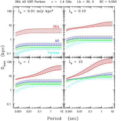
Figure 6: Plot of $D_{\rm max}$ vs. $P$ for surveys at 1.4 GHz using the Parkes 64-m antenna, Arecibo, and the SKA, as labelled, and the Green Bank Telescope (unlabelled). The four panels correspond to different pseudo-luminosities $L_{\rm p}$. In each panel a band is shown for each telescope, the top corresponding to full gain and the bottom to partial gain. For the SKA, the partial gain is due to only $f_{c}=0.25$ of the array being available for pulsar searches. For the other telescopes, the bottom band boundary is for 0.5 of the peak gain. Parameters used for the SKA, Arecibo, GBT and Parkes, respectively, are as follows. Bandwidth: 0.4, 0.3, 0.4 and 0.3 GHz; Integration time: 3600, 300, 900 and 2100 sec; Number of channels: 1024, 1024, 1024 and 96; Time constant: 64, 64, 64 and 250 $\mu$s; SEFD: 0.14, 3.6, 16 and 40 Jy. In all cases, a 10$\sigma$ detection threshold for the harmonic sum of a Fourier spectrum is assumed. The decline at small periods is due to smearing of pulses from a combination of receiver time resolution and propagation effects (dispersion and scattering). This effect is larger for the Parkes Multibeam survey which used wide spectrometer channels, thus allowing more dispersive pulse smearing. With 1024 channels, dispersion is largely unimportant while pulse broadening from scattering limits $D_{\rm max}$ for short periods. periods. The results show that the SKA can detect pulsars at distances 2 to 10 times larger than with Arecibo and can probe to reasonable distances even for luminosities $L_{\rm p}\mathbin{\lower 3.0pt\hbox{$\hbox to0.0pt{\raise 5.0pt\hbox{$\char 60\relax$}\hss}\mathchar 29208\relax$}}0.01$ mJy kpc² that are currently inaccessible. For $L_{\rm p}=10$ mJy kpc², the SKA can reach 100 kpc for longer periods. Given that some pulsars have $L_{\rm p}>10^{3}$ mJy kpc² at 1.4 GHz, it is clear the the SKA can reach distances $>1$ Mpc in periodicity searches.

Single-pulse searches: Searches for giant pulses can be made in both blind and targeted searches. Because they differ from periodicity searches only in the Fourier analysis part of the latter, the same requirements on numbers of channels, total bandwidth and overall sensitivity apply.

4.2 Targeted Observations

In addition to regular timing observations discussed in §4.3 and possible VLBI measurements of their astrometric parameters (§4.4), many pulsars will also require dedicated targeted observations to achieve the various science goals. However, most of the requirements of targeted observations are identical to those for search and timing measurements. Indeed, nearly all aspects of the outlined science programmes have in common that they require multi-frequency observations. These are necessary to study the broad-band emission of pulsars, to correct for propagation effects on the pulsed signal, and for studies of the interstellar medium itself. It is therefore desirable that the SKA has constant broad frequency coverage, and at the least the SKA should be able to change frequency on a regular and rapid ($\sim$ minutes) basis.

For some of science goals, such as the study of relativistic plasma physics (§3.4), simultaneous multi-frequency observations with full polarization capabilities are required, often over frequency ranges much greater than a few GHz. This simultaneity can be achieved in different ways with the SKA, depending on the actual design. Assuming that SKA frontends are made up of a number of different classes of receiver, each designed to cover a different frequency range, simultaneous multi-frequency coverage can be achieved through the ability of all of the receivers in each of the different classes to be operated simultaneously giving full sensitivity at all wavelengths. Alternatively, the SKA could form sub-arrays of receivers from different frequencies up to some limited total number of receivers. Whilst this second option still provides the desired simultaneity, it clearly results in a loss of total sensitivity.

4.3 Timing Measurements

Timing observations require faster sampling of the frequency-time plane than search observations because the time-tagging of pulses is desired to high accuracy. At minimum, dedispersion must be done as completely as possible, requiring either coherent dedispersion of baseband signals sampled before detection or post-detection dedispersion with a large number of channels across the measured bandwidth. Sample times needed are $\mathbin{\lower 3.0pt\hbox{$\hbox to0.0pt{\raise 5.0pt\hbox{$\char 60\relax$}\hss}\mathchar 29208\relax$}}1\,\mu s$ for millisecond pulsars, the objects of greatest interest.

Timing Precision Issues: Phenomena that limit time-of-arrival (TOA) precision include ([13])

1. Radiometer noise, which yields an rms variation

   $${\sigma_{\rm TOA}}_{,n} \simeq \frac{W}{P(S/N)}$$ (9)

   $$\simeq \frac{WS_{\rm sys}}{\langle S\rangle\sqrt{2BT}}\left(\frac{W}{P}\right)^{1/2},$$

   where $S/N$ is the signal to noise ratio of the pulse peak in a sample pulse profile and $W$ is the pulse width (FWHM, in time units).

2. Pulse phase jitter, which occurs in the vast majority of pulsars as drifting sub-pulses and apparently random jumps accompanied by large amplitude variations having a modulation index $m_{\rm I}=$ rms/mean $\sim 1$. Quantifying the rms jitter of a single pulses as a fraction $f_{\rm j}$ of the pulse width $W$, the rms TOA variation is

   $${\sigma_{\rm TOA}}_{,j}\simeq\frac{1}{2}\epsilon_{i}^{-1/2}f_{\rm j}(1+m_{\rm I}^{2})^{1/2}W\left(\frac{P}{T}\right)^{1/2},$$ (10)

   where $\epsilon_{i}\leq 1$ measures the fraction of the pulses in the observation time $T$ that are statistically independent. Phase jitter without intensity modulation ($m_{\rm I}=0$) produces a TOA error but the converse is not true.

3. Scattering-induced variations include the systematic delay associated with pulse broadening (c.f. §2.2), which can vary with epoch, and timing variations associated with the finite number of “scintles” (patches of constructive interference) in the frequency-time plane. Closely related are DM-variations associated with large-scale electron-density fluctuations (AU to pc; [1]) and variations in angle of arrival caused by large-scale gradients. Together, this collection of effects associated with the dispersion relation for cold plasma in the ISM yields several contributions with different frequency scaling, ranging from $\nu^{-2}$ to $\nu^{-4.4}$ [26].

4. Pulse Polarization can induce TOA errors from incorrect gain calibration and from instrumental polarization. For a Gaussian pulse of width $W$, the induced TOA error from gain variation is

   $${\sigma_{\rm TOA}}_{\rm,pol}=\frac{\epsilon\pi_{\rm V}W}{2\sqrt{2\ln 2}},$$ (11)

   where $\epsilon$ is the fractional gain error on the circularly polarized channels ($\delta g/g=\epsilon$) and $\pi_{\rm V}$ is the degree of circular polarization. For $\epsilon=\pi_{\rm V}=0.1$ and $W=$ 1 ms, the error is 4.2 $\mu$s, for example. If there is no circular polarization, the error vanishes. If the receiver polarization channels are linearly polarized, a similar error ensues. Instrumental polarization such as cross coupling in the feed can induce false circular polarization $\pi_{\rm V}\simeq 2\eta^{1/2}\pi_{\rm L}$, where $\pi_{\rm L}$ is the degree of linear polarization, which is often quite high in pulsars, and $\eta$ is the voltage cross coupling coefficient. Combined with gain errors, the pseudo-V yields a TOA error as above. To achieve better than 100 ns timing precision, one must have $\epsilon\eta^{1/2}\pi_{\rm L}\mathbin{\lower 3.0pt\hbox{$\hbox to0.0pt{\raise 5.0pt\hbox{$\char 60\relax$}\hss}\mathchar 29208\relax$}}10^{-4}W_{\rm ms}^{-1}$, for a pulse width of $W_{\rm ms}$ ms. If the gain precision is 1%, this requires cross coupling $\eta\mathbin{\lower 3.0pt\hbox{$\hbox to0.0pt{\raise 5.0pt\hbox{$\char 60\relax$}\hss}\mathchar 29208\relax$}}10^{-4}$, corresponding to a net polarization purity of $-40$dB. This may be achieved through good antenna and feed performance and post-processing calibration. Similar numbers will hold for linearly polarized feeds, though it is generally advisable for measurements on pulsars, which are elliptically polarized, to be made with circularly polarized feeds.

To obtain optimised arrival times, the above scaling laws imply that observations with the highest sensitivity are needed to minimize the radiometer noise contribution and thus favour lower frequencies (except for pulsars with shallow spectra). Phase jitter, whose strength (${\sigma_{\rm TOA}}_{,j}$) varies greatly from pulsar to pulsar, is nearly independent of frequency and can be minimised only with longer dwell times on a pulsar. Phase jitter begins to dominate the contribution from radiometer noise when S/N $\sim 1$ for a single pulse for the case where $f_{\rm j}=1$. For at least one MSP, $f_{\rm j}\ll 1$ [21], so that phase jitter may be less important. In general, however, high-sensitivity measurements with the SKA will yield TOAs dominated by phase jitter and systematic errors from polarization and gain-calibration effects. Contributions from propagation effects clearly imply that high frequencies are favoured. The overall optimal frequency is highly pulsar dependent and thus requires that the SKA provide a wide range of frequencies, extending to at least $\sim 5$ GHz. Moreover, timing measurements at multiple frequencies allow ISM effects to be partially removed.

While precision polarization and gain calibrations are required in order to obtain the best TOAs, the ability to sample the frequency-time plane with adequate resolution to identify individual scintillation features is also required to correct for some of the perturbations to TOAs. The effective observing time needed per pulsar to get a precise TOA measurement will, however, depend on the individual pulsar, i.e. as to whether radiometer or pulse-phase jitter contributions to the TOA uncertainty are dominant.

Multiple Beaming and Multiple Fields of View: Given the large number of weak sources to be discovered among the $\sim 20,000$ pulsars to be timed, the capability to observe multiple pulsars simultaneously, either through multiple beams within the same FOV or by using multiple FOVs, is clearly desirable. Along the Galactic plane we expect $\mathbin{\lower 3.0pt\hbox{$\hbox to0.0pt{\raise 5.0pt\hbox{$\char 60\relax$}\hss}\mathchar 29208\relax$}}100$ sources per 1-deg² FOV while as many beams should also be sufficient to sample the denser populated regions. However, most 1-deg² FOVs will contain only a few pulsars, so that larger FOVs or several independently steerable FOVs would be beneficial.

In a worst case analysis, one can estimate from simulations that with only four independent 1-deg² FOVs, one needs $\sim 50$ days of observing time with full-SKA sensitivity to get one TOA measurement for all discovered pulsars. Assuming that the main contribution to TOA errors for MSPs is given by radiometer noise, a high S/N TOA measurement for all $\sim 1000$ MSPs would still require $\sim 10-20$ days with full SKA sensitivity. Access to only reduced SKA sensitivity and limited simultaneous multi-frequency coverage will increase the needed observing time correspondingly while observations on similar or even more frequent intervals are clearly necessary to achieve some of the key science goals. However, in reality, optimisation procedures, such as the choice of lower frequencies above the Galactic plane or the selection of fewer but more precise MSPs, will reduce the demand on observing time. Nevertheless, given the necessity to allow the SKA also to be used for other key science programmes, a larger number of independently covered FOVs of the sky appears essential.

4.4 VLBI Observations

The scientific motivation for obtaining VLBI observations of pulsars is three-fold. Firstly, from the requirements of the strong-field gravity key-science project, it is clear that uncertainties in a pulsar’s distance and motion limit the accuracy to which kinematic corrections can be applied to observables like the orbital period derivative and hence to which precision tests of theories of gravity can be performed (see §3.1). Secondly, pulsar parallaxes provide key calibration constraints into models of the Galactic electron density. Even a relatively small number of parallaxes can provide crucial constraints on the distribution of the interstellar medium near the Sun [78]. Finally, proper motions are essential for estimating pulsar velocities, which in turn provide constraints on the supernova collapse mechanism (see §3.10).

VLBI observations require finding an optimal frequency that balances astrometric accuracy, pulsar spectra, and atmospheric and ionospheric phase fluctuations. Pulsar spectra generally favor observations at lower frequencies ($\mathbin{\lower 3.0pt\hbox{$\hbox to0.0pt{\raise 5.0pt\hbox{$\char 60\relax$}\hss}\mathchar 29208\relax$}}1$ GHz), but ionospheric phase fluctuations become significant and the lower resolution attainable (e.g., 5 mas on terrestrial baselines) vitiate astrometry at these frequencies. Higher frequencies provide higher astrometric accuracy and reduced ionospheric phase fluctuations at the cost of a reduced sample size because of the steep spectra.

We anticipate that the SKA’s sensitivity will provide a broad optimization for VLBI observations in the approximate frequency range of 2–8 GHz. Ionospheric phase fluctuations are reduced at these frequencies while tropospheric phase fluctuations are not yet severe. Transcontinental/intercontinental baselines provide resolutions of order 3 mas, and sub-milliarcsecond astrometric accuracies are being obtained already [9]. A key aspect of the SKA’s sensitivity will be its role in finding calibrators/phase reference sources close to target pulsars. Chatterjee et al. (2004) have demonstrated that astrometric accuracy depends strongly upon the separation between the calibrator and target source.

If 10% of the SKA’s collecting area is spread over transcontinental/intercontinental baselines, it would be some 20 times more sensitive than current dedicated VLBI arrays. This improved sensitivity not only increases the sample of pulsars available for astrometric purposes but also increases the density of background sources to serve as phase reference sources. Finally, we emphasize the importance of dedicated VLBI capabilities for pulsar astrometry. Ad-hoc VLBI arrays can be constructed today with collecting areas approaching $10^{5}$ m². By their very nature, though, these arrays are difficult to maintain for the multi-year durations required for astrometric projects.

4.5 Summary

The outlined requirements are summarized in Table 1 where we quote the required temporal resolution, sensitivity and frequency coverage, alongside with comments on the required configuration, Field-of-View (FOV) sampling and polarization capabilities.

Table 1: Summary of SKA specifications required for the various parts of the pulsar science case.

Topic	Required Specification
	$\delta t$	$A/T$	$\nu_{\mathrm{max}}$	Configuration	FOV Sampling	Polarization
	($\mu$s)	(m2/K)	(GHz)			(output, isolation)
Searching
Galactic Census	50	$f_{c}$ 20,000	2.5	“core,” with large $f_{c}$	full	Total
Galactic Center	50	$f_{c}$ 20,000	15	“core,” with large $f_{c}$	full	Total
Extragalactic	50	$f_{c}$ 20,000	1.5	“core,” with large $f_{c}$	full	Total
Globular Clusers	50	$f_{c}$ 20,000	1.5	“core,” with large $f_{c}$	full	Total
Targeted	50	$f_{c}$ 20,000	1.5	“core,” with large $f_{c}$	full	summed
Timing
GR tests, NS-BH binaries,	$<1$	20,000	15	non-critical if phasable	100 beams/deg2	full Stokes, $-40$dB
MSPs
GR tests, Galactic center	100	20,000	15	non-critical if phasable	10 beams/deg2	full Stokes, $-40$dB
NS-BH binaries
VLBI
gated astrometry	200	$>2000$	8	intercontinental baselines	$\sim 3$ beams	Total
(proper motion, parallax)

5 Conclusions

Given the richness and diversity of the outlined science case, the research on pulsars conducted since their discovery appears to be only the prelude to what will be possible with the Square Kilometer Array. As for other areas in modern astronomy, the SKA will revolutionise the field of pulsar astrophysics. The SKA will enable not only the discovery of most pulsars in the Milky Way but also allows present-day-survey sensitivities to pulsars in the closest Galaxies. With the single-pulse search techniques, it should be possible to detect giant pulses from pulsars as distant as the Virgo Cluster. The impressive yield of 10,000 to 20,000 discovered pulsars, including over 1,000 millisecond pulsars, effectively samples every possible outcome of the evolution of massive binary stars, thereby guaranteeing the discovery of very exciting systems. We expect at least 100 compact relativistic binaries, including the elusive pulsar-black hole systems. For tests of theories of gravity of general relativity such a system could well surpass all present and foreseeable competitors. It may be possible through pulsar timing to precisely determine the mass, spin and quadrupole moment of the black hole (see contribution by Kramer et al., this volume). Such measurements would go beyond what is currently possible with binary pulsar tests of general relativity, perhaps even confronting Einstein’s famous “no-hair” theorem for black holes. The structure of the Milky Way and its magnetic field can be studied in far greater detail than presently possible, particularly with the expected increase in parallax measurements made possible by the SKA’s superior sensitivity. In addition, studies of the significant numbers of extragalactic pulsars expected to be detectable by the SKA would allow measurements of the intergalactic, as opposed to the interstellar, medium.

References

- [1] D. C. Backer, S. Hama, S. van Hook,& R. S. Foster, ApJ, 404, (1993), 636-642.
- [2] M. Bailes, S. M. Ord, H. S. Knight, A. W. Hotan, ApJ 595 (2003) L49–L52.
- [3] M. G. Baring, A. K. Harding, ApJ 507 (1998) L55–L58.
- [4] B. M. Barker, R. F. O’Connell, Phys. Rev. D 12 (1975) 329–335.
- [5] C. A. Beichman, in: Proc. SPIE Vol. 3350, p. 719-723, Astronomical Interferometry, Robert D. Reasenberg; Ed., 1998, pp. 719–723.
- [6] D. Bhattacharya & E. P. J. van den Heuvel, Physics Reports, 203, (1991), 1-124.
- [7] M. Burgay, N. D’Amico, A. Possenti, R. N. Manchester, A. G. Lyne, B. C. Joshi, M. McLaughlin, M. Kramer, J. M. Sarkissian, F. Camilo, V. Kalogera, C. Kim, D. R. Lorimer, Nature 426 (2003) 531–533.
- [8] F. Camilo, V. M. Kaspi, A. G. Lyne, R. N. Manchester, J. F. Bell, N. D’Amico, N. P. F. McKay, F. Crawford, ApJ 541 (2000) 367–373.
- [9] S. Chatterjee, J. M. Cordes, W. H. T. Vlemmings, Z. Arzoumanian, W. M. Goss, T. J. W. Lazio, ApJ 604 (2004) 339–345.
- [10] K. S. Cheng, C. Ho, M. Ruderman, ApJ 300 (1986) 500–521.
- [11] I. Cognard, J. A. Shrauner, J. H. Taylor, S. E. Thorsett, ApJ 457 (1996) L81–L84.
- [12] Colpi, M., M. Mapelli, & A. Possenti, Astrophysical Journal, 599, (2003), 1260-1271.
- [13] J. M. Cordes, in: J. A. Phillips, S. E. Thorsett, S. R. Kulkarni (Eds.), Planets around Pulsars, Astron. Soc. Pac. Conf. Ser. Vol. 36, 1993, pp. 43–60.
- [14] J. M. Cordes, T. J. W. Lazio, ApJSubmitted astro-ph/0207156.
- [15] J. M. Cordes, T. J. W. Lazio, ApJSubmitted astro-ph/0301598.
- [16] T. Damour, G. Schäfer, Nuovo Cim. 101 (1988) 127.
- [17] T. Damour, J. H. Taylor, Phys. Rev. D 45 (1992) 1840–1868.
- [18] T. Damour, G. Esposito-Farèse, Phys. Rev. D 58 (042001) (1998) 1–12.
- [19] S. Detweiler, ApJ 234 (1979) 1100–1104.
- [20] O. V. Doroshenko, S. M. Kopeikin, MNRAS 274 (1995) 1029.
- [21] R. T. Edwards, B. W. Stappers, A&A 407 (2003) 273–287.
- [22] Emmering, R. T.& R. A. Chevalier, Astrophysical Journal, 345, (1989), 931-938.
- [23] G. Esposito-Farese, In: Proceedings of the 10th Marcel Grossmann meeting, 2004, contribution to 10th Marcel Grossmann meeting, gr-qc/0402007.
- [24] F. R. Ferraro, A. Possenti, E. Sabbi, P. Lagani, R. T. Rood, N. D’Amico, L. Origlia, ApJ 595 (2003) 179–186.
- [25] R. S. Foster, D. C. Backer, ApJ 361 (1990) 300.
- [26] R. S. Foster, J. M. Cordes, ApJ 364 (1990) 123–135.
- [27] P. C. Freire, M. Kramer, A. G. Lyne, F. Camilo, R. N. Manchester, N. D’Amico, ApJ 557 (2001) L105–L108.
- [28] P. C. Freire, F. Camilo, M. Kramer, D. R. Lorimer, A. G. Lyne, R. N. Manchester, N. D’Amico, MNRAS 340 (2003) 1359–1374.
- [29] G. Gonzalez, MNRAS 285 (1997) 403–412.
- [30] J. E. Grindlay, F. Camilo, C. O. Heinke, P. D. Edmonds, H. Cohn, P. Lugger, ApJ 581 (2002) 470–484.
- [31] Gürkan, M. A., M. Freitag, & F. A. Rasio, Astrophysical Journal, 604, (2004), 632-652.
- [32] T. H. Hankins, J. S. Kern, J. C. Weatherall, J. A. Eilek, Nature 422 (2003) 141–143.
- [33] W. E. Harris, AJ 112 (1996) 1487–1488.
- [34] E. R. Harrison, E. Tademaru, ApJ 201 (1975) 447–461.
- [35] A. Hewish, S. J. Bell, J. D. H. Pilkington, P. F. Scott, R. A. Collins, Nature 217 (1968) 709–713.
- [36] F. A. Jenet, A. Lommen, S. L. Larson, L. Wen, American Astronomical Society Meeting 203.
- [37] S. Johnston, R. W. Romani, ApJ 590 (2003) L95–98.
- [38] P. Kaaret, ApJ 578 (2002) 114–125.
- [39] V. Kalogera, C. Kim, D. R. Lorimer, M. Burgay, N. D’Amico, A. Possenti, R. N. Manchester, A. G. Lyne, B. C. Joshi, M. A. McLaughlin, M. Kramer, J. M. Sarkissian, F. Camilo, ApJ 601 (2004) L179–L182.
- [40] A. Karastergiou, A. von Hoensbroech, M. Kramer, D. Lorimer, A. Lyne, O. Doroshenko, A. Jessner, A. Jordan, R. Wielebinski, A&A 379 (2001) 270–278.
- [41] D. Koch, W. Borucki, J. J. Lissauer, E. W. Dunham, J. Jenkins, Bulletin of the American Astronomical Society 30 (1998) 1058.
- [42] M. Konacki, A. Wolszczan, ApJ 591 (2003) L147–L150.
- [43] S. M. Kopeikin, G. Schäfer, Phys. Rev. D 60 (1999) 124002.
- [44] S. Kopeikin, in: . S. T. M. Bailes, D. Nice, S. Thorsett (Ed.), Radio Pulsars (ASP Conf. Ser.), PASP, San Francisco, 2003, p. 111.
- [45] M. Kramer, A. G. Lyne, G. Hobbs, O. Lohmer, P. Carr, C. Jordan, A. Wolszczan, ApJ 593 (2003) 31.
- [46] M. Kramer, K. M. Xilouris, A. Jessner, D. R. Lorimer, R. Wielebinski, A. G. Lyne, A&A 322 (1997) 846–856.
- [47] D. Lai, D. F. Chernoff, J. M. Cordes, ApJ 549 (2001) 1111–1118.
- [48] T. J. W. Lazio, J. M. Cordes, ApJ 505 (1998) 715–731.
- [49] A. N. Lommen, D. C. Backer, ApJ 562 (2001) 297–302.
- [50] D. R. Lorimer, M. Bailes, R. J. Dewey, P. A. Harrison, MNRAS 263 (1993) 403–415.
- [51] A. G. Lyne, M. Burgay, M. Kramer, A. Possenti, R. N. Manchester, F. Camilo, M. McLaughlin, D. R. Lorimer, B. C. Joshi, J. E. Reynolds, P. C. C. Freire, Science 303 (2004) 1153–1157.
- [52] M. A. McLaughlin, I. H. Stairs, V. M. Kaspi, D. R. Lorimer, M. Kramer, A. G. Lyne, R. N. Manchester, F. Camilo, G. Hobbs, A. Possenti, N. D’Amico, A. J. Faulkner, ApJ 591 (2003) L135–L138.
- [53] D. B. Melrose, in: M. Kramer, N. Wex, R. Wielebinski (Eds.), Pulsar Astronomy - 2000 and Beyond, IAU Colloquium 177, Astronomical Society of the Pacific, San Francisco, 2000, p. 721.
- [54] Merritt, D., S. Piatek, S. P. Zwart, & M. Hemsendorf, Astrophysical Journal, 608, (2004), L25-L28.
- [55] Moffett, D. A. and Hankins, T. H., ApJ 468 (1996) 779–783.
- [56] J. R. Oppenheimer, G. Volkoff, Phys. Rev. 55 (1939) 374–381.
- [57] P. C. Peters, Rev. 136 (1964) 1224–1232.
- [58] E. Pfahl, A. Loeb,
- [59] S. Phinney, J. H. Taylor, Nature 277 (1979) 117–118.
- [60] M. Rajagopal, R. W. Romani, ApJ 446 (1995) 543–549.
- [61] H. B. Richer, R. Ibata, G. G. Fahlman, M. Huber, ApJ 597 (2003) L45–L47.
- [62] R. Romani, S. Johnston, ApJ 557 (2001) L93.
- [63] N. C. Santos, G. Israelian, M. Mayor, A&A 373 (2001) 1019–1031.
- [64] R. Schödel, T. Ott, R. Genzel, R. Hofmann, M. Lehnert, A. Eckart, N. Mouawad, T. Alexander, M. J. Reid, R. Lenzen, M. Hartung, F. Lacombe, D. Rouan, E. Gendron, G. Rousset, A.-M. Lagrange, W. Brandner, N. Ageorges, C. Lidman, A. F. M. Moorwood, J. Spyromilio, N. Hubin, K. M. Menten, Nature 419 (2002) 694–696.
- [65] U. J. Schwarz, J. D. Bregman, J. H. van Gorkom, A&A 215 (1989) 33–47.
- [66] S. L. Shapiro, S. A. Teukolsky, Wiley–Interscience, New York, 1983.
- [67] A. Shearer, B. Stappers, P. O’Connor, A. Golden, R. Strom, M. Redfern, O. Ryan, Science 301 (2003) 493–495.
- [68] S. Sigurdsson, H. B. Richer, B. M. Hansen, I. H. Stairs, S. E. Thorsett, Science 301 (2003) 193–196.
- [69] S. L. Shemar, A. G. Lyne, MNRAS 282 (1996) 677–690.
- [70] I. S. Shklovskii, Sov. Astron. 13 (1970) 562–565.
- [71] D. N. Spergel, Nature 352 (1991) 221–222.
- [72] I. H. Stairs, A. G. Lyne, S. Shemar, Nature 406 (2000) 484–486.
- [73] I. H. Stairs, Living Reviews in Relativity 6 (2003) 5.
- [74] I. H. Stairs, Science 304 (2004) 547–552.
- [75] J. H. Taylor, L. A. Fowler, P. M. McCulloch, Nature 277 (1979) 437.
- [76] D. J. Thompson, Advances in Space Research 25 (2000) 659–668.
- [77] D. J. Thompson, in: S. Johnston, M. A. Walker, M. Bailes (Eds.), Pulsars: Problems and Progress, IAU Colloquium 160, Astronomical Society of the Pacific, San Francisco, 1996, pp. 307–314.
- [78] M. Toscano, M. C. Britton, R. N. Manchester, M. Bailes, J. S. Sandhu, S. R. Kulkarni, S. B. Anderson, ApJ 523 (1999) L171–L175.
- [79] A. G. J. van Leeuwen, B. W. Stappers, R. Ramachandran, J. M. Rankin, A&A 399 (2003) 223–229.
- [80] W. van Straten, M. Bailes, M. Britton, S. R. Kulkarni, S. B. Anderson, R. N. Manchester, J. Sarkissian, Nature 412 (2001) 158–160.
- [81] W. van Straten, Ph.D. thesis, Swinburne University of Technology (2003).
- [82] J. M. Weisberg, J. H. Taylor, in: M. Bailes, D. J. Nice, S. Thorsett (Eds.), Radio Pulsars, Astronomical Society of the Pacific, San Francisco, 2003, pp. 93–98.
- [83] N. Wex, Phd thesis, Ph.D. thesis, Jena University, Jena, Germany (1995).
- [84] N. Wex, J. Gil, M. Sendyk, A&A 311 (1996) 746–757.
- [85] N. Wex, Quantum Grav. 12 (1995) 983.
- [86] A. Wolszczan, D. A. Frail, Nature 355 (1992) 145–147.